A dynamic nonstationary spatio-temporal model for short term prediction of precipitation

Abstract

Precipitation is a complex physical process that varies in space and time. Predictions and interpolations at unobserved times and/or locations help to solve important problems in many areas. In this paper, we present a hierarchical Bayesian model for spatio-temporal data and apply it to obtain short term predictions of rainfall. The model incorporates physical knowledge about the underlying processes that determine rainfall, such as advection, diffusion and convection. It is based on a temporal autoregressive convolution with spatially colored and temporally white innovations. By linking the advection parameter of the convolution kernel to an external wind vector, the model is temporally nonstationary. Further, it allows for nonseparable and anisotropic covariance structures. With the help of the Voronoi tessellation, we construct a natural parametrization, that is, space as well as time resolution consistent, for data lying on irregular grid points. In the application, the statistical model combines forecasts of three other meteorological variables obtained from a numerical weather prediction model with past precipitation observations. The model is then used to predict three-hourly precipitation over 24 hours. It performs better than a separable, stationary and isotropic version, and it performs comparably to a deterministic numerical weather prediction model for precipitation and has the advantage that it quantifies prediction uncertainty.

, and

1 Introduction

Precipitation is a very complex phenomenon that varies in space and time, and there are many efforts to model it. Predictions and interpolations at unobserved times and/or locations obtained from such models help to solve important problems in areas such as agriculture, climate science, ecology and hydrology. Stochastic models have the great advantage of providing not only point estimates, but also quantitative measures of uncertainty. They can be used, for instance, as stochastic generators [Wilks (1998), Makhnin and McAllister (2009)] to provide realistic inputs to flooding, runoff and crop growth models. Moreover, they can be applied as components within general circulation models used in climate change studies [Fowler et al. (2005)], or for postprocessing precipitation forecasts [Sloughter et al. (2007)].

1.1 Distributions for precipitation

A characteristic feature of precipitation is that its distribution consists of a discrete component, indicating occurrence of precipitation, and a continuous one, determining the amount of precipitation. As a consequence, there are two basic statistical modeling approaches. The continuous and the discrete part are either modeled separately [Coe and Stern (1982), Wilks (1999)] or together [Bell (1987), Wilks (1990), Bardossy and Plate (1992), Hutchinson (1995), Sansó and Guenni (2004)]. Typically, in the second approach, the distribution of the rainfall amounts and the probability of rainfall are determined together using what is called a censored distribution. Originally, this idea goes back to Tobin (1958) who analyzed household expenditure on durable goods. For modeling precipitation, Stidd (1973) took up this idea and modified it by including a power-transformation for the nonzero part so that the model can account for skewness.

1.2 Correlations in space and time

For modeling processes that involve dependence over space and time, there are two basic approaches [see, e.g., Cressie and Wikle (2011)]: one which models the space–time covariance structure without distinguishing between the time and space dimensions, and a dynamic one which takes the natural ordering in the time dimension into account.

The first approach usually follows the traditional geostatistical paradigm of assuming a parametric covariance function [for an introduction into geostatistics, see, e.g., Cressie (1993) or Gelfand et al. (2010)]. Several parametric families specifying explicitly the joint space–time covariance structure have been proposed [Jones and Zhang (1997), Cressie and Huang (1999), Gneiting (2002), Ma (2003), Stein (2005), Paciorek and Schervish (2006)]. Interpretability and, especially, computational complexity are challenges when working with parametric space–time covariance functions.

There is, however, a fundamental difference between the spatial and the temporal dimensions. Whereas there is an order in the time domain, there exists no obvious order for space. It is therefore natural to assume a dynamic temporal evolution combined with a spatially correlated error term [Sølna and Switzer (1996), Wikle and Cressie (1999), Huang and Hsu (2004), Xu, Wikle and Fox (2005), Gelfand, Banerjee and Gamerman (2005)]. As Wikle and Hooten (2010) state, the dynamic approach can be used to construct realistic space–time dependency structures based on physical knowledge. Further, the temporal Markovian structure offers computational benefits.

1.3 Models for precipitation

Isham and Cox (1994) state that there are three broad types of mathematical models of rainfall: deterministic meteorological models [Mason (1986)], intermediate stochastic models [Le Cam (1961), Cox and Isham (1988), Waymire, Gupta and Rodriguez-Iturbe (1984)], and empirical statistical models. Meteorological models represent as realistically as possible the physical processes involved. As noted by Kyriakidis and Journel (1999), deterministic models typically require a large number of input parameters that are difficult to determine, whereas stochastic models are usually based on a small number of parameters. Nevertheless, statistical models can also incorporate knowledge about physical processes. Parametrizations can be chosen based on physical knowledge and covariates reflecting information about the physical processes can be included.

In the following, we briefly review statistical models for precipitation. For modeling daily precipitation at a single measuring site, Stern and Coe (1984) use a nonstationary second-order Markov chain to describe precipitation occurrence and a gamma distribution to describe rainfall amounts. Hughes and Guttorp (1994) and Hughes, Guttorp and Charles (1999) model precipitation occurrence using a nonhomogeneous hidden Markov model. With the help of an unobserved weather state they link large scale atmospheric circulation patterns with the local precipitation process. Bellone, Hughes and Guttorp (2000) and Charles, Bates and Hughes (1999) both extend this approach by also modeling precipitation amounts. The former propose to use gamma distributions, whereas the latter use empirical distribution functions. Ailliot, Thompson and Thomson (2009) present a hidden Markov model in combination with the transformed and censored Gaussian distribution approach used in Bardossy and Plate (1992). Also building on the same censoring idea, Sansó and Guenni (1999a) model precipitation occurrence and amount of precipitation using a transformed multivariate Gaussian model with a spatial correlation structure. Further works on statistical precipitation modeling include Sansó and Guenni (1999b, 2000), Brown et al. (2001), Stehlik and Bardossy (2002), Allcroft and Glasbey (2003), Sloughter et al. (2007), Berrocal, Raftery and Gneiting (2008) and Fuentes, Reich and Lee (2008).

1.4 Outline

The model presented in the following is a hierarchicalBayesian model for spatio-temporal data. At the data stage, we opt for a modeling approach that determines the discrete and the continuous parts of the precipitation distribution together. This is done by assuming the existence of a latent Gaussian variable which can be interpreted as a precipitation potential. The mean of the Gaussian variable is related to covariates through a regression term. The advantages of this one-part modeling strategy are twofold: the model contains less parameters and it can deal with the so-called spatial (and temporal) intermittence effect [Bardossy and Plate (1992)] which suggests smooth transitions between wet and dry areas. This means that at the edge of a dry area the amount of rainfall should be low. Wilks (1998) notes that, indeed, lower rainfall intensity is observed when more neighboring stations are dry. This feature also reflects the idea that if a model determines a low probability of rainfall for a given situation, it should also give a small expected value for its amount conditional on this event, and vice versa. However, we note that there is no consensus in the literature whether the two parts of precipitation should be modeled together or separately.

At the process level, we use a dynamic model for accounting for spatio-temporal variation. The model explicitly incorporates knowledge about the underlying physical processes that determine rainfall, such as advection, diffusion and convection. Approximating an integrodifference equation, we obtain a temporally autoregressive convolution with spatially colored and temporally white innovations. The model is nonstationary, anisotropic, and it allows for nonseparable covariance structures, that is, covariance structures where spatial and temporal variation interact. While our approach builds on existing models, it includes several novel features. With the help of the Voronoi tessellation, a natural parametrization for data lying on an irregular grid is obtained. The parametrization based on this tessellation is space as well as time resolution consistent, physically realistic and allows for modeling irregularly spaced data in a natural way. To our knowledge, the use of the Voronoi tessellation for spatio-temporal data on an irregular grid is new. By linking the advection parameter of the kernel to an external wind vector, the model is temporally nonstationary.

The model is applied to predict three-hourly precipitation. The prediction model is based on three forecasted meteorological variables obtained from an NWP model as well as past rainfall observations. We compare predictions from the statistical model with the precipitation forecasts obtained from the NWP.

The remainder is organized as follows. In Section 2 the model specifications are presented. In Section 3 it is shown how the model can be fitted to data using a Markov chain Monte Carlo (MCMC) algorithm and how predictions can be obtained. Next, in Section 4 the model is applied to obtain short term predictions of three-hourly rainfall. Conclusions are given in Section 5.

2 The model

It is assumed that the rainfall $Y_{t}({\mathbf{s}})$ at time $t$ on site ${\mathbf{s}}=(x,y)^{\prime}\in\mathbb{R}^{2}$ depends on a latent normal variable $W_{t}({\mathbf{s}})$ through

$$Y_{t}({\mathbf{s}}) = 0\qquad\mbox{if }W_{t}({\mathbf{s}})\leq 0$$

$$= W_{t}({\mathbf{s}})^{\lambda}\qquad\mbox{if }W_{t}({\mathbf{s}})>0,$$

where $\lambda>0$. A power transformation is needed since precipitation amounts are more skewed than a truncated normal distribution and since the scatter of the precipitation amounts increases with the average amount. The latent variable $W_{t}({\mathbf{s}})$ can be interpreted as a precipitation potential.

This latent variable $W_{t}({\mathbf{s}})$ is modeled as a Gaussian process that is specified as

$$W_{t}({\mathbf{s}})={\mathbf{x}}_{t}({\mathbf{s}})^{T}{\bolds\beta}+\xi_{t}({\mathbf{s}})+\nu_{t}({\mathbf{s}}),$$ (2)

where $\bolds{\beta}\in\mathbb{R}^{k}$, and $\nu_{t}({\mathbf{s}})\sim N(0,\tau^{2}),\tau^{2}>0$, are i.i.d. The mean ${\mathbf{x}}_{t}({\mathbf{s}})^{T}{\bolds\beta}$ of $W_{t}({\mathbf{s}})$ is assumed to depend linearly on regressors ${\mathbf{x}}_{t}({\mathbf{s}})\in\mathbb{R}^{k}$. For notational convenience, we split the terms specifying the covariance function into a structured part $\xi_{t}({\mathbf{s}})$ and an unstructured “nugget” $\nu_{t}({\mathbf{s}})$. The term $\xi_{t}({\mathbf{s}})$ is a zero-mean Gaussian process that accounts for structured variation in time and space. It is specified below in Section 2.1. The nugget $\nu_{t}({\mathbf{s}})$ models microscale variability and measurement errors. Since, typically, the resolution of the data does not allow for distinguishing between microscale variability and measurement errors, we model these two sources of variation together. Note that the covariates ${\mathbf{x}}_{t}({\mathbf{s}})$ will usually be time and location dependent. In addition to weather characteristics, Fourier harmonics can be included to account for seasonality, and functions of coordinates can account for smooth effects in space.

2.1 The convolution autoregressive model

We follow the dynamic approach and define an explicit time evolution through the following integrodifference equation (IDE):

$$\xi_{t}({\mathbf{s}})=\int_{\mathbb{R}^{2}}{h_{{\bolds\vartheta}}\bigl{(}{\mathbf{s}}-{\mathbf{s}}^{\prime}\bigr{)}\xi_{t-1}\bigl{(}{\mathbf{s}}^{\prime}\bigr{)}\,d{\mathbf{s}}^{\prime}}+\varepsilon_{t}({\mathbf{s}}),\qquad{\mathbf{s}}\in\mathbb{R}^{2},$$ (3)

where $\varepsilon_{t}({\mathbf{s}})$ is a Gaussian innovation that is white in time and colored in space, and $h_{{\bolds\vartheta}}$ is a Gaussian kernel,

$$h_{{\bolds\vartheta}}\bigl{(}{\mathbf{s}}-{\mathbf{s}}^{\prime}\bigr{)}=\phi\exp\bigl{(}-\bigl{(}{\mathbf{s}}-{\mathbf{s}}^{\prime}-{\bolds\mu}_{t}\bigr{)}^{T}{\bolds\Sigma}^{-1}\bigl{(}{\mathbf{s}}-{\mathbf{s}}^{\prime}-{\bolds\mu}_{t}\bigr{)}\bigr{)},$$ (4)

where the parameter vector ${{\bolds\vartheta}}$ combines $\phi$ and the elements of ${\bolds\mu}_{t}$ and ${\bolds\Sigma}^{-1}$. Note that ${\bolds\mu}_{t}$ shifts the kernel and ${\bolds\Sigma}^{-1}$ determines the range and the degree of anisotropy. The parameter $\phi$ controls the amount of temporal correlation. More details on the interpretation of the model and specific choices of the parameters ${\bolds\mu}_{t}$ and ${\bolds\Sigma}$ are discussed below in Section 2.2. An illustration of this kernel can be found in the application in Section 4.2.

In the following, we assume that we have $N$ measurement locations ${\mathbf{s}}_{i}$, $i=1,\ldots,N$, where measurements are made at times $t=1,\ldots,T$. Instead of working with a fine spatial grid with many missing observations, we formulate an approximate model for the values at the stations only, ${\bolds\xi}_{t}=(\xi_{t}({\mathbf{s}}_{1}),\ldots,\xi_{t}({\mathbf{s}}_{N}))^{\prime}$. Discretizing the integral in (3), we obtain

$$\int_{\mathbb{R}^{2}}h_{{\bolds\vartheta}}\bigl{(}{\mathbf{s}}_{i}-{\mathbf{s}}^{\prime}\bigr{)}\xi_{t-1}\bigl{(}{\mathbf{s}}^{\prime}\bigr{)}\,d{\mathbf{s}}^{\prime} \approx \int_{A}h_{{\bolds\vartheta}}\bigl{(}{\mathbf{s}}_{i}-{\mathbf{s}}^{\prime}\bigr{)}\xi_{t-1}\bigl{(}{\mathbf{s}}^{\prime}\bigr{)}\,d{\mathbf{s}}^{\prime}$$

$$\approx \sum_{j=1}^{N}{h_{{\bolds\vartheta}}({\mathbf{s}}_{i}-{\mathbf{s}}_{j})\xi_{t-1}({\mathbf{s}}_{j})|A_{j}|}.$$

Here $A\subset\mathbb{R}^{2}$ is an area which contains the convex hull of all stations, the sets $A_{i},i=1,\ldots,N$, form a tessellation of $A$ with ${\mathbf{s}}_{i}\in A_{i}$ and $|A_{j}|$ denotes the area of cell $A_{j}$.

Our model can then be written as the vector autoregression

$${\bolds\xi}_{t}=\phi{\mathbf{G}}_{t}{\bolds\xi}_{t-1}+{\bolds\varepsilon}_{t},\qquad{\mathbf{G}}_{t}\in\mathbb{R}^{N\times N},$$ (6)

where

$$({\mathbf{G}}_{t})_{ij}=\exp\bigl{(}-\bigl{(}{\mathbf{s}_{i}}-{\mathbf{s}}_{j}^{\prime}-{\bolds\mu}_{t}\bigr{)}^{T}{\bolds\Sigma}^{-1}\bigl{(}{\mathbf{s}}_{i}-{\mathbf{s}}_{j}^{\prime}-{\bolds\mu}_{t}\bigr{)}\bigr{)}\cdot|A_{j}|,$$ (7)

and where ${\bolds\varepsilon}_{t}=(\varepsilon_{t}({\mathbf{s}}_{1}),\ldots,\varepsilon_{t}({\mathbf{s}}_{N}))^{\prime}$.

Note that this process does not exhibit explosive growth if the largest eigenvalue of $\phi{\mathbf{G}}_{t}$ is smaller than one. To ensure this, we check in our application that the largest eigenvalue is smaller than one for the parameters at the posterior modes.

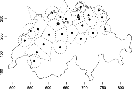
Figure 1: Locations of stations. Both axes are in km using the Swiss coordinate system (CH1903). The lines illustrate the Voronoi tessellation. Cells with unbounded area have been replaced by circles whose area is determined as described in the text.

If the ${\mathbf{s}}_{i}$’s form a regular grid, a tessellation is straightforward. Otherwise, we propose to use the Voronoi tessellation [Voronoi (1908)] which decomposes the space. Specifically, each site ${\mathbf{s}}_{i}$ has a corresponding Voronoi cell consisting of all points closer to ${\mathbf{s}}_{i}$ than to any other site ${\mathbf{s}}_{j}$, $j\neq i$ [see, e.g., Okabe et al. (2000) for more details]. Stations on the boundary of the convex hull have cells with infinite area. For these stations, we define $|{A}_{i}|$ as described in the following. We first calculate the Voronoi tessellation of $\mathbb{R}^{2}$. We then replace unbounded cells by cells whose area is the average area of the neighboring bounded cells. In Figure 1, the Voronoi tessellation for the Swiss stations used in the application below is shown as an example. Concerning the stations on the boundary, the circles represent the surface area $|{A}_{i}|$.

As mentioned before, the ${\bolds\varepsilon}_{t}$’s are assumed to be independent over time and colored in space. More precisely, we assume a stationary, isotropic Gaussian random field

$${\bolds\varepsilon}_{t}\sim N\bigl{(}0,\sigma^{2}{\mathbf{V}}_{\rho_{0}}\bigr{)},\qquad\sigma^{2}>0,$$ (8)

with

$${({\mathbf{V}}_{\rho_{0}})}_{ij}=\exp(-d_{ij}/\rho_{0}),\qquad\rho_{0}>0,\qquad 1\leq i,j,\leq N,$$ (9)

where $d_{ij}$ denotes the Euclidean distance between two sites $i$ and $j$. The exponential correlation function is used for computational convenience. In principle, it is possible to use other covariance functions, for instance, other members of the Matérn family.

The approximation in (2.1) assumes that $h_{{\bolds\vartheta}}$ is approximately constant in each cell. If some cells are considered to be too large for this approximation to be reasonable, additional points ${\mathbf{s}}_{j}^{\ast}$ can be added for which all observations are missing. Since such additional points increase the computational load, some compromise has to be found between accuracy and computational feasibility.

2.2 Interpretation and parametrization of the kernel function

For the purpose of interpretation, we note that, in the limit when the temporal spacing goes to zero, the solution of the IDE (3) can also be written as the solution of the stochastic partial differential equation (SPDE) [see Brown et al. (2000)]

$$\frac{\partial}{\partial t}\xi_{t}({\mathbf{s}})=-{\bolds\mu}_{t}\cdot\nabla\xi_{t}({\mathbf{s}})+\frac{1}{4}\nabla\cdot{\bolds\Sigma}\nabla\xi_{t}({\mathbf{s}})-\eta\xi_{t}({\mathbf{s}})+B_{t}({\mathbf{s}}),$$ (10)

where $\nabla=(\frac{\partial}{\partial x},\frac{\partial}{\partial y})$ is the gradient operator and where $B_{t}({\mathbf{s}})$ is temporally independent and spatially dependent. The terms have the following interpretations: ${\bolds\mu}_{t}\cdot\nabla\xi_{t}({\mathbf{s}})$ models advection, ${\bolds\mu}_{t}$ being a drift or velocity vector. The second term is a diffusion term that can incorporate anisotropy, and $-\eta\xi_{t}({\mathbf{s}})$ accounts for damping. The damping parameter $\eta$ is related to $\phi$ and ${\bolds\Sigma}$ through $\eta=-\log(\phi\pi|{\bolds\Sigma}|^{1/2})$. $B_{t}({\mathbf{s}})$ is a source-sink or stochastic forcing term that can be interpreted as modeling convective phenomena. This interpretation is based on the reasoning that typically convective precipitation cells emerge and cease on the domain of interest in contrast to larger scale advective precipitation that is being transported over the area.

We now turn to the discussion of the parameterization of ${\bolds\mu}_{t}$ and ${\bolds\Sigma}$. In our application, we have information about wind. It is assumed that the drift term ${\bolds\mu}_{t}$ is proportional to this external wind vector. With ${\bolds\mu}_{t}$ varying over time, the model is temporally nonstationary. It is also conceivable that in certain situations ${\bolds\Sigma}$ or $\eta$ may vary over time and/or space, thus obtaining different forms of nonstationarity. Concerning ${\bolds\Sigma}$, it is thought that potential anisotropy is related to topography. Denoting by ${\mathbf{w}}_{t}$ the wind vector at time $t$, we assume

$${\bolds\mu}_{t} = u\cdot{\mathbf{w}}_{t}\quad\mbox{and}$$

$${\bolds\Sigma}^{-1} = \frac{1}{\rho_{1}^{2}}\pmatrix{\cos{\alpha}&\sin{\alpha}\cr-c\cdot\sin{\alpha}&c\cdot\cos{\alpha}}^{T}\pmatrix{\cos{\alpha}&\sin{\alpha}\cr-c\cdot\sin{\alpha}&c\cdot\cos{\alpha}},$$

where $u\in\mathbb{R}$, $c>0$, and $\alpha\in[0,\pi/2]$. We use a wind vector which is averaged over the entire area, but the wind could also change locally. The motivation for writing ${\bolds\Sigma}$ in the given form comes from considering a coordinate transformation

$$\pmatrix{x^{\prime}\cr y^{\prime}}=\pmatrix{\cos{\alpha}&\sin{\alpha}\cr-c\cdot\sin{\alpha}&c\cdot\cos{\alpha}}\pmatrix{x\cr y},$$ (12)

where the parameter $\alpha$ is the angle of rotation, and $c$ determines the degree of anisotropy, $c=1$ corresponding to the isotropic case. $\rho_{1}$ is a range parameter that determines the degree of interaction between spatial and temporal correlation. See Section 4.2 for an illustration of a kernel with the above parametrization.

The resulting model is nonstationary and incorporates anisotropy. Finally, we note that there are various other possible choices of parametrizations. For instance, a relatively simple model can be obtained by assuming

$${\bolds\mu}_{t}={\mathbf{0}}\quad\mbox{and}\quad{\bolds\Sigma}^{-1}=\frac{1}{\rho_{1}^{2}}\pmatrix{1&0\cr 0&1},$$ (13)

that is, no drift and an isotropic diffusion term. There is still spatio-temporal interaction, though, which implies that the model is not separable in the sense that (16) does not hold. We can simplify further and take not only ${\bolds\mu}_{t}={\mathbf{0}}$, but also ${\bolds\Sigma}={\mathbf{0}}$, leading to ${\mathbf{G}}_{t}$ being the identity matrix

$${\bolds\xi}_{t}=\phi{\bolds\xi}_{t-1}+{\bolds\varepsilon}_{t}.$$ (14)

This means that each point at time $t-1$ only has an influence on itself at time $t$, that is, there is no spatio-temporal interaction and the model is separable.

2.3 Discussion of the model

Propagator matrix ${\mathbf{G}}_{t}$. Using a parametrized propagator matrix ${\mathbf{G}}_{t}$ in (6) has the obvious advantage that less parameters are needed than in the general case, in which each entry in the matrix has to be estimated, resulting in $N^{2}$ parameters. Moreover, in contrast to the general case, the parametric approach allows for making predictions at sites where no measurements are available, which is often of interest in applications.

Space resolution consistency. At first sight, it might be tempting to use a simpler parametrization of ${\mathbf{G}}_{t}$ not based on a convolution but of the form

$$({\mathbf{G}}_{t})_{ij}=\exp\bigl{(}-(d_{ij}/\rho_{1})^{2}\bigr{)}.$$ (15)

However, such a model has the following important drawback. Assume, for instance, that a station $i$ is surrounded by two neighboring sites $j$ and $k$. Say that both stations $j$ and $k$ lie at the same distance from $i$ but in different directions. Consequently, $j$ and $k$ at time $t-1$ exercise the same influence on $i$ at time $t$. If one adds an additional station $l$ very close to $k$, the joint influence of $k$ and $l$ at time $t-1$ on site $i$ at time $t$ would then approximately be twice as big as the one of site $j$. This means that the distribution of the process at point $i$ depends on the number and the location of stations in the neighborhood at which it has been observed. The convolution model, on the other hand, does not exhibit this drawback. Furthermore, the convolution model has the advantage that it is “space resolution consistent,” that is, it retains approximately its temporal Markovian structure if one, or several, sites are removed from the domain. This does not hold true for the simpler vector autoregressive model as specified in (15).

Space–time covariance structure. In the following, let us turn to the spatio-temporal dependence structure of the latent process ${\bolds\xi}_{t}$. A random field $\xi_{t}({\mathbf{s}})$, $({\mathbf{s}},t)\in\mathbb{R}^{2}\times\mathbb{R}$ is said to have a separable covariance structure [Gneiting, Genton and Guttorp (2007)] if there exist purely spatial and purely temporal covariance functions $C_{S}$ and $C_{T}$, respectively, such that

$$\mbox{cov}\bigl{(}\xi_{t_{1}}({\mathbf{s}}_{1}),\xi_{t_{2}}({\mathbf{s}}_{2})\bigr{)}=C_{S}({\mathbf{s}}_{1},{\mathbf{s}}_{2})\cdot C_{T}(t_{1},t_{2}).$$ (16)

The convolution based approach allows for nonseparable covariance structures, whereas the separable autoregressive model in (14) has a separable covariance structure.

Extremal events. For the data model as specified in equation (2), Hernández, Guenni and Sansó (2009) showed that the distribution of the maxima is a Gumbel. If the focus lies on extremal events, other distributions, which have Fréchet maxima, can be used, for instance, a $t$-distribution. The $t$-distribution is particularly attractive since it is a scale mixture of normal distributions. To be more specific, if $S_{t}$ has a $\chi_{df}^{2}$ distribution, then ${\mathbf{W}}_{t}={\mathbf{x}}_{t}^{T}{\bolds\beta}+({\bolds\xi}_{t}+{\bolds\nu}_{t})/\sqrt{S_{t}/df}$ has a multivariate $t$-distribution. This means that the fitting algorithm introduced below can be extended to the $t$-distribution case by introducing an additional latent variable $S_{t}$.

3 Fitting and prediction

Fitting is done using a Markov chain Monte Carlo method (MCMC), the Metropolis–Hastings algorithm [Metropolis et al. (1953), Hastings (1970)]. Concerning most parameters, it will be shown that the full conditionals are known distributions. Therefore, Gibbs sampling [Gelfand and Smith (1990)] can be used in these cases.

For convenience and later use, we combine the parameters characterizing the model into a vector ${\bolds\theta}=(\lambda,{\bolds\beta}^{\prime},\tau^{2},\sigma^{2},\rho_{0},{\bolds\vartheta}^{\prime})^{\prime}$ and call them primary parameters. Our goal is to simulate from the joint posterior distribution of these parameters and the latent variables ${\bolds\xi}=({\bolds\xi}_{1},\ldots,{\bolds\xi}_{T}),{\bolds\xi}_{0}$, and ${\mathbf{W}}=({\mathbf{W}}_{1},\ldots,{\mathbf{W}}_{T})$. We note that those $W_{t}({\mathbf{s}}_{i})$ that correspond to observed values above zero are known. In that case the full conditional distribution consists of a Dirac distribution at $Y_{t}({\mathbf{s}}_{i})^{1/\lambda}$. For handling the censored values and for allowing for missing values, we adopt a data augmentation approach [Smith and Roberts (1993)] as specified below in equation (3.1). See Section 3.1 for more details.

Assuming prior independence among the primary parameters, the prior distributions are specified as

$$P\bigl{[}\lambda,\bolds{\beta},\tau^{2},\sigma^{2},\rho_{0},\phi,u,\rho_{1},\alpha,c,{\bolds\xi}_{0}\bigr{]}$$

(17)

$$\qquad\propto\frac{1}{\tau^{2}}\frac{1}{\sigma^{2}}P[\rho_{0}]P[\rho_{1}]P[u]P[c]P[\alpha]P\bigl{[}{\bolds\xi}_{0}|\sigma^{2},\rho_{0}\bigr{]}$$

with ${\bolds\xi}_{0}$ having a normal prior $P[{\bolds\xi}_{0}|\sigma^{2},\rho_{0}]=N(0,\sigma^{2}{\mathbf{V}}_{\rho_{0}})$. Further, $\rho_{0}$ and $\rho_{1}$ have gamma priors with mean $\mu_{\rho}$ and variance $\sigma^{2}_{\rho}$. For $c$, we assume a gamma prior with mean $1$ and variance $1$, $\alpha$ has a uniform prior on $[0,\pi/2]$, and $u$ has a normal prior with mean $0$ and variance $10^{4}$. Further, we assume locally uniform priors on $\log(\tau^{2})$ and $\log(\sigma^{2})$ as well as for $\phi$, $\lambda$ and ${\bolds\beta}$.

In our application, we choose to use informative priors for $\rho_{0}$ and $\rho_{1}$. It is known that in model-based geostatistics difficulties can arise when estimating the variance and scale parameters of the exponential covariogram [see, e.g., Warnes and Ripley (1987), Mardia and Watkins (1989), Diggle, Tawn and Moyeed (1998)]. For the geostatistical covariance model, Zhang (2004) shows that the product of the two parameters can be estimated consistently, and Stein (1990) shows that it is the product of the two parameters that matters more than the individual parameters for spatial interpolation. Further, Berger, De Oliveira and Sansó (2001) show that, at least in the simplest setting, the posterior of the range parameters is improper for most noninformative priors. Given these considerations, we think that using informative priors for the two range parameters $\rho_{0}$ and $\rho_{1}$ is appropriate. In our example, we chose priors with mean $\mu_{\rho}=100$ and variance $\sigma^{2}_{\rho}=10$. We have tried different informative priors. The less informative they are, the worse are the mixing properties of the MCMC algorithm. In line with the results of Stein (1990) and Zhang (2004), we have made the experience that different choices of priors on these range parameters do not have a strong impact on the predictive performance of the model.

The posterior distribution is then proportional to

$$\biggl{(}\frac{1}{\sigma^{2}}\biggr{)}^{{N(T+1)}/{2}+1}\biggl{(}\frac{1}{\tau^{2}}\biggr{)}^{{NT}/{2}+1}|{\mathbf{V}}_{\rho_{0}}|^{-({T+1})/{2}}\prod_{Y_{t}({\mathbf{s}}_{i})>0}\frac{Y_{t}({\mathbf{s}}_{i})^{1/\lambda-1}}{\lambda}$$

$$\qquad{}\times\exp\Biggl{(}-\frac{1}{2}\sum_{t=1}^{T}\frac{1}{\tau^{2}}\bigl{\|}{\mathbf{W}}_{t}-{\mathbf{x}}_{t}^{T}{\bolds\beta}-{\bolds\xi}_{t}\bigr{\|}^{2}$$

(18)

$$\qquad\hskip 34.5pt{}+\frac{1}{\sigma^{2}}({\bolds\xi}_{t}-\phi{\mathbf{G}}_{t}{\bolds\xi}_{t-1})^{\prime}{\mathbf{V}}_{\rho_{0}}^{-1}({\bolds\xi}_{t}-\phi{\mathbf{G}}_{t}{\bolds\xi}_{t-1})\Biggr{)}$$

$$\qquad{}\times\exp\biggl{(}-\frac{1}{2}\frac{1}{\sigma^{2}}{\bolds\xi}_{0}^{\prime}{\mathbf{V}}_{\rho_{0}}^{-1}{\bolds\xi}_{0}\biggr{)}\cdot P[\rho_{0}]\cdot P[{\bolds\vartheta}]\cdot\mathbf{1}_{\{W_{t}({\mathbf{s}}_{i})\leq 0\ \forall i,t\dvtx Y_{t}({\mathbf{s}}_{i})=0\}}.$$

The product in the first line is the Jacobian for the power transformation in (2). Note that missing observations do not cause any problem. If $Y_{t}({\mathbf{s}}_{i})$ is missing, there is no respective term in the product nor a corresponding condition for the indicator function.

3.1 Full conditional distributions

In the following, we derive full conditional distributions for the individual parameters.

It is readily seen that the full conditional of ${\bolds\beta}$ is a multivariate normal distribution, and the full conditional distribution of $\phi$ is a normal distribution as well. The full conditionals of both $\sigma^{2}$ and $\tau^{2}$ are inverse gamma distributions.

For obtaining the full conditionals of ${\mathbf{W}}_{t}$, we partition its components according to whether $Y_{t}({\mathbf{s}}_{i})$ is above zero, equal to zero, or missing. Denote by $i_{t}^{[+]}$ those indices for which $Y_{t}({\mathbf{s}}_{i})>0$, by $i_{t}^{[0]}$ those with $Y_{t}({\mathbf{s}}_{i})=0$, and by $i_{t}^{[m]}$ the missing ones. The vector ${\mathbf{W}}_{t}$ can then be partitioned into ${\mathbf{W}}_{t}^{[+]}$, ${\mathbf{W}}_{t}^{[0]}$, and ${\mathbf{W}}_{t}^{[m]}$ accordingly. We remark that ${\mathbf{W}}_{t}^{[0]}$ and ${\mathbf{W}}_{t}^{[m]}$ are latent variables, whereas ${\mathbf{W}}_{t}^{[+]}$ corresponds to transformed observed values. In addition, ${\mathbf{W}}_{t}^{[0]}$ has the restriction that all its values must be smaller than zero, ${\mathbf{W}}_{t}^{[0]}\leq{\mathbf{0}}$. For facilitating understanding, we note that $W_{t}({\mathbf{s}}_{i})$ can be written as

$$W_{t}({\mathbf{s}}_{i}) = W_{t}^{[+]}({\mathbf{s}}_{i})=Y_{t}({\mathbf{s}}_{i})^{1/\lambda}\qquad\mbox{if }Y_{t}({\mathbf{s}}_{i})>0$$

$$= W_{t}^{[0]}({\mathbf{s}}_{i})\qquad\mbox{if }Y_{t}({\mathbf{s}}_{i})=0$$

$$= W_{t}^{[m]}({\mathbf{s}}_{i})\qquad\mbox{if }Y_{t}({\mathbf{s}}_{i})\mbox{ is missing}.$$

The full conditional of ${\mathbf{W}}_{t}^{[m]}$ is then a multivariate normal distribution with mean and covariance

$$\mu_{{\mathbf{W}}_{t}^{[m]}}=\bigl{(}{\mathbf{x}}_{t}^{T}{\bolds\beta}+{\bolds\xi}_{t}\bigr{)}^{[m]}\quad\mbox{and}\quad{\bolds\Sigma}_{{\mathbf{W}}_{t}^{[m]}}=\tau^{2}\cdot{\mathbf{I}}.$$ (20)

Similarly, the full conditional distribution of ${\mathbf{W}}_{t}^{[0]}$ is a truncated multivariate normal distribution with mean and covariance

$$\mu_{{\mathbf{W}}_{t}^{[0]}}=\bigl{(}{\mathbf{x}}_{t}^{T}{\bolds\beta}+{\bolds\xi}_{t}\bigr{)}^{[0]}\quad\mbox{and}\quad{\bolds\Sigma}_{{\mathbf{W}}_{t}^{[0]}}=\tau^{2}\cdot{\mathbf{I}}.$$ (21)

As mentioned before, the full conditional of ${\mathbf{W}}_{t}^{[+]}$ is a Dirac distribution with point mass at $({\mathbf{Y}}_{t}^{[+]})^{1/\lambda}$.

Concerning the latent variables $({\bolds\xi}_{0},{\bolds\xi}_{1},\ldots,{\bolds\xi}_{T})$, we note that conditional on ${\bolds\theta}$, $({\bolds\xi}_{t},{\mathbf{W}}_{t})$ is a linear Gaussian state space model. Therefore, a sample from the joint full conditional of $({\bolds\xi}_{0},{\bolds\xi}_{1},\ldots,{\bolds\xi}_{T})$ can be obtained using the forward filtering backward sampling (FFBS) algorithm proposed by Carter and Kohn (1994) and Frühwirth-Schnatter (1994). The forward filtering step corresponds to the Kalman filter [see, e.g., West and Harrison (1997) and Künsch (2001)].

Alternatively, one can also use single $t$ updates. The full conditional of one ${\bolds\xi}_{t}$, $0\leq t\leq T$, is a normal distribution $N({\bolds\mu}_{{\bolds\xi}_{t}},{\bolds\Sigma}_{{\bolds\xi}_{t}})$. In the case of the separable model, the mean ${\bolds\mu}_{{\bolds\xi}_{t}}$ depends on ${\bolds\xi}_{t-1}$ and ${\bolds\xi}_{t+1}$, whereas the covariance matrix ${\bolds\Sigma}_{{\bolds\xi}_{t}}$ does not depend on $t$. This is convenient for simulation since its Cholesky decomposition has to be calculated only once in each update cycle. In contrast, in the sampling step of the FFBS algorithm, one has to calculate a Cholesky decomposition for each $t$. The advantage that the FFBS algorithm mixes better than the single $t$ update algorithm per update cycle is outweighed by the fact that an update cycle of the single $t$ update algorithm is a lot faster than one of the FFBS algorithm. Thus, more effective samples can be obtained with the single $t$ update algorithm per time. In the case of the nonstationary anisotropic drift model, though, ${\bolds\Sigma}_{{\bolds\xi}_{t}}$ in the single $t$ update algorithm is not constant over time. Thus, a Cholesky decomposition needs to be computed for each $t$ anyway, meaning that the FFBS algorithm is preferable.

In summary, we made the experience that it is recommendable to use single $t$ updates for temporally stationary models where the covariance ${\bolds\Sigma}_{{\bolds\xi}_{t}}$ of the full conditional of one ${\bolds\xi}_{t}$ is constant over time. If ${\bolds\Sigma}_{{\bolds\xi}_{t}}$ changes over time, we recommend using the FFBS algorithm.

For the remaining parameters, that is, $\rho_{0}$, ${\bolds\vartheta}$ (excluding $\phi$) and $\lambda$, there is no apparent distribution family from which one can simulate. Therefore, Metropolis steps will be used. We note that the full conditional distribution of $\lambda$ is proportional to

$$\quad\prod_{Y_{t}({\mathbf{s}}_{i})>0}\biggl{(}\frac{Y_{t}({\mathbf{s}}_{i})^{1/\lambda-1}}{\lambda}\biggr{)}\exp\biggl{(}-\frac{1}{2}\sum_{Y_{t}({\mathbf{s}}_{i})>0}\frac{1}{\tau^{2}}\bigl{\|}Y_{t}({\mathbf{s}}_{i})^{1/\lambda}-{\mathbf{x}}_{t}^{T}{\bolds\beta}-{\bolds\xi}_{t}\bigr{\|}^{2}\biggr{)}.$$ (22)

The parameter $\lambda$ is sampled on the log-scale. This means that we first transform it to the log scale. Then a proposal is obtained by sampling from a normal distribution with the mean equal to the last value of the parameter. Thereafter, this proposal is accepted with a probability that is given by the usual Metropolis–Hasting algorithm [see, e.g., Chib and Greenberg (1995)].

Finally, $\rho_{0}$ and ${\bolds\vartheta}$ (excluding $\phi$) are sampled together. The full conditional is proportional to

$$\exp\Biggl{(}-\frac{1}{2\sigma^{2}}\Biggl{(}\sum_{t=1}^{T}({\bolds\xi}_{t}-\phi{\mathbf{G}}_{t}{\bolds\xi}_{t-1})^{\prime}{\mathbf{V}}_{\rho_{0}}^{-1}({\bolds\xi}_{t}-\phi{\mathbf{G}}_{t}{\bolds\xi}_{t-1})+{\bolds\xi}_{0}^{\prime}{\mathbf{V}}_{\rho_{0}}^{-1}{\bolds\xi}_{0}\Biggr{)}\Biggr{)}$$

(23)

$$\qquad{}\times|{\mathbf{V}}_{\rho_{0}}|^{-({T+1})/{2}}.$$

3.2 Prediction

We consider predictions at new locations and/or times as well as predictions of areal averages. It turns out that in the case of areal averages, the Voronoi tessellation is again useful.

One way to obtain predictions is to augment the data ${\mathbf{Y}}_{\mathrm{obs}}$ with missing values at the locations or times where predictions are made. When doing so, the MCMC algorithm implicitly draws from the corresponding predictive distribution. See the previous Section 3.1 on how to handle missing values.

If one does not specify the points in space and time where predictions are to be made prior to model fitting, the predictive distribution of a new set of observations ${\mathbf{Y}}^{*}=(Y^{*}_{t^{*}_{1}}({\mathbf{s}}^{*}_{1}),\ldots,Y^{*}_{t^{*}_{k}}({\mathbf{s}}^{*}_{k}))^{\prime}$ is calculated as

$$P\bigl{[}{\mathbf{Y}}^{*}|{\mathbf{Y}}_{\mathrm{obs}}\bigr{]} = \int P\bigl{[}{\mathbf{Y}}^{*}|{\bolds\xi}^{*},{\bolds\theta}\bigr{]}P\bigl{[}{\bolds\xi}^{*}|{\bolds\xi},{\bolds\theta}\bigr{]}P[{\bolds\xi},{\bolds\theta}|{\mathbf{Y}}_{\mathrm{obs}}]\,d{\bolds\xi}^{*}\,d{\bolds\xi}\,d{\bolds\theta}$$

$$\approx \frac{1}{m}\sum_{i=1}^{m}\int P\bigl{[}{\mathbf{Y}}^{*}|{\bolds\xi}^{*},{\bolds\theta}^{(i)}\bigr{]}P\bigl{[}{\bolds\xi}^{*}|{\bolds\xi}^{(i)},{\bolds\theta}^{(i)}\bigr{]}\,d{\bolds\xi}^{*}$$

$$\approx \frac{1}{m}\sum_{i=1}^{m}P\bigl{[}{\mathbf{Y}}^{*}|{\bolds\xi}^{*(i)},{\bolds\theta}^{(i)}\bigr{]},$$

where ${\mathbf{Y}}_{\mathrm{obs}}$ denotes the observed data, ${\bolds\xi}$ and ${\bolds\xi}^{*}$ the latent Gaussian process at the observed and predicted sites, respectively, and ${\bolds\theta}$ all the remaining parameters. Samples ${\bolds\theta}^{(i)}$ and ${\bolds\xi}^{(i)},i=1,\ldots,m$, from their posterior distribution are obtained by the MCMC algorithm, and ${\bolds\xi}^{*(i)}$ is sampled from $P[{\bolds\xi}^{*}|{\bolds\xi}^{(i)},{\bolds\theta}^{(i)}]$.

When ${\bolds\xi}^{*}$ is modeled at the same sites as ${\bolds\xi}$ but at different time points, the distribution $P[{\bolds\xi}^{*}|{\bolds\xi}^{(i)},{\bolds\theta}^{(i)}]$ is Gaussian and readily obtained using (6).

In the case when predictions are made at unobserved sites $s\in S$ and time $t$, $P[{\bolds\xi}_{t}^{*}|{\bolds\xi},{\bolds\theta}]$ can be calculated as described in the following. First, because of the temporal Markov property, $P[{\bolds\xi}_{t}^{*}|{\bolds\xi},{\bolds\theta}]$ is equal to $P[{\bolds\xi}_{t}^{*}|{\bolds\xi}_{t-1},{\bolds\xi}_{t},{\bolds\xi}_{t+1},{\bolds\theta}]$. This density is then obtained by considering the augmented model

$$\pmatrix{{\bolds\xi}_{t}\cr{\bolds\xi}_{t}^{*}} = \phi\pmatrix{{\mathbf{G}}_{t}\cr{\mathbf{G}}^{*}_{t}}{\bolds\xi}_{t-1}+\pmatrix{{\bolds\varepsilon}_{t}\cr{\bolds\varepsilon}_{t}^{*}},$$

$${\bolds\xi}_{t+1} = \phi\bigl{(}\matrix{{\mathbf{H}}_{t+1}&{\mathbf{H}}_{t+1}^{*}}\bigr{)}\pmatrix{{\bolds\xi}_{t}\cr{\bolds\xi}_{t}^{*}}+{\bolds\varepsilon}_{t+1},$$

where ${\mathbf{G}}^{*}_{t}$ is defined analogously to (7), ${\mathbf{H}}_{t+1}$ and ${\mathbf{H}}_{t+1}^{*}$ are obtained from the same approximations as in (2.1), and the covariances of ${\bolds\varepsilon}_{t}$ and ${\bolds\varepsilon}_{t}^{*}$ are as in (9). By (3.2), the conditional distribution of ${\bolds\xi}_{t},{\bolds\xi}_{t}^{*},{\bolds\xi}_{t+1}$ given ${\bolds\xi}_{t-1}$ is normal. Therefore, also the conditional distribution of ${\bolds\xi}_{t}^{*}$ given ${\bolds\xi}_{t-1},{\bolds\xi}_{t},{\bolds\xi}_{t+1}$ is Gaussian. Its mean and covariance can be computed by noting that

$$P\bigl{[}{\bolds\xi}_{t}^{*}|{\bolds\xi}_{t-1},{\bolds\xi}_{t},{\bolds\xi}_{t+1},{\bolds\theta}\bigr{]} \propto P\bigl{[}{\bolds\xi}_{t+1}|{\bolds\xi}_{t}^{*},{\bolds\xi}_{t},{\bolds\theta}\bigr{]}P\bigl{[}{\bolds\xi}_{t}^{*}|{\bolds\xi}_{t-1},{\bolds\xi}_{t},{\bolds\theta}\bigr{]}$$

$$\propto P\bigl{[}{\bolds\xi}_{t+1}|{\bolds\xi}_{t}^{*},{\bolds\xi}_{t},{\bolds\theta}\bigr{]}P\bigl{[}{\bolds\xi}_{t},{\bolds\xi}_{t}^{*}|{\bolds\xi}_{t-1},{\bolds\theta}\bigr{]}$$

and then completing the square in the exponent of the last expression.

In many cases, for instance, when the focus lies on flooding, areal averages

$$\bar{Y}^{(A^{*})}_{t}=\frac{1}{|A^{*}|}\int_{A^{*}}Y_{t}({\mathbf{s}})\,d{\mathbf{s}}$$ (27)

of precipitation are of interest. If $Y_{t}({\mathbf{s}})$ is observed on an irregular grid, one could first define a regular grid, then interpolate the nonobserved grid points, and approximate the integral in (27) by a Riemann sum. However, since the regular grid usually becomes very large, this is computationally expensive. Instead, we propose to use the Voronoi tessellation once again to approximate the integral

$$\bar{Y}^{(A^{*})}_{t}=\frac{1}{|A^{*}|}\int_{A^{*}}Y_{t}({\mathbf{s}})\,d{\mathbf{s}}\approx\frac{1}{|A^{*}|}\sum_{j=1}^{N}Y_{t}({\mathbf{s}}_{j})\bigl{|}A_{j}\cap A^{*}\bigr{|}.$$ (28)

Thereby, an adequate weight $|A_{j}\cap A^{*}|$ is given to each station. Samples from the predictive distribution of $\bar{Y}^{(A^{*})}_{t}$ can be obtained by simulating $Y^{(i)}_{t}({\mathbf{s}}_{j})$ from their predictive distribution and inserting them in (28).

We note that the areal prediction becomes deterministic if all $Y_{t}({\mathbf{s}}_{j})$ consist of observed values. This means that uncertainty about values of $Y_{t}({\mathbf{s}})$ at locations where no observations are made is implicitly ignored with the above approximation. This can be amended for by first making predictions at a few sites where no observations were made. Inserting additional unobserved sites can also be useful in other cases. For instance, if $A^{*}$ cuts off a substantial part of any $A_{j}$, that is, $A_{j}\cap A^{*}$ is much smaller than $A_{j}$ but not empty, the areal prediction might be improved by replacing $Y_{t}({\mathbf{s}}_{j})$ by the prediction of $Y_{t}$ at the center of gravity of $A_{j}\cap A^{*}$, or if the area $A^{*}$ is small and contains only a few stations, improved predictions of the areal average can be obtained by making predictions at a few additional points inside the area.

4 Application to short term prediction of precipitation

We apply the model to obtain short term forecasts of precipitation. Such forecasts are important, for instance, for agriculture and flooding. The traditional way for obtaining precipitation forecasts is the use of numerical weather prediction (NWP) models. NWP models solve complex, nonlinear equations emulating the dynamics of the atmosphere. Typically, NWP models require a lot of computational resources to run. Fitting our statistical model using the MCMC algorithm presented above is also computationally intensive. However, once the statistical model is fitted and assuming that the posterior of the primary parameters does not change (see Section 4.3 for more details), predictions are computationally a lot cheaper. Furthermore, the statistical model can be used in situations where there are no NWP models available or to obtain predictions at different temporal resolutions than the one at which the NWP model operates.

4.1 The data

The data consists of three-hourly precipitation amounts collected by 26 stations around the Swiss Plateau from the beginning of December 2008 to the end of March 2009, making a total of $968$ time periods. The data were provided by MeteoSwiss. We use the first three months, consisting of $720$ time periods, for fitting the model. The remaining month March, consisting of $248$ time periods, is

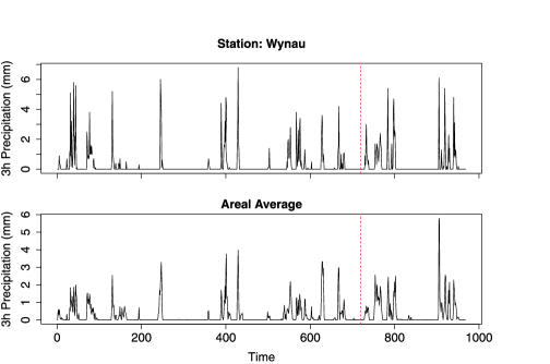
Figure 2: Precipitation versus time. The lines are observed precipitation of one station (corresponding to the station with the acronym WYN in Figure 1) and of the areal average. The time axis is in 3 h steps starting at December 1, 2008. The dotted vertical line separates the training and test data.

set aside for model evaluation. The locations of these stations are shown in Figure 1. In Figure 2, a time series plot of the observed precipitation at one station (corresponding to the station with the acronym WYN in Figure 1) and of the weighted areal average is shown. Concerning the latter, we take the weighted average over the entire spatial domain. Figure 3 shows the spatial distribution of the precipitation accumulated over time.

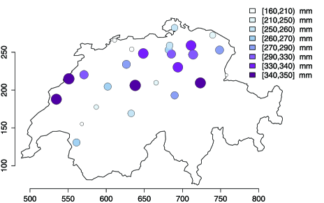
Figure 3: Illustration of the spatial distribution of precipitation. The circles display the cumulative rainfall amounts over time at the stations. The larger the circle and the darker the color, the higher is the cumulative precipitation amount. Both axes are in km.

The covariates consist of the x- and y-coordinates (km), altitude (m), temperature (^∘C), dew point (^∘C) and specific humidity ($\%$). Specific humidity is the ratio of water vapor to dry air in a particular mass. It is expected to be positively related to precipitation. The dew point is the temperature to which a given parcel of humid air must be cooled, at constant barometric pressure, for water vapor to condense into water. Thus, the lower the dew point, the lower is the chance for precipitation. However, specific humidity and dew point are considerably negatively correlated. This makes it unclear, a priori, what their joint relation to precipitation is like. Temperature, dew point and specific humidity are predicted variables obtained from an NWP model called COSMO-2. From the same model, we also obtain wind predictions (speed is in m/s). Predictions of the statistical model are evaluated by comparing them to precipitation forecasts from the same NWP. Having a high resolution with a grid spacing of 2.2 km, the NWP model is able to resolve convective dynamics. The NWP model produces predictions once a day for 24 hours ahead starting at 0:00UTC. After assimilation and computation, forecasts are available at around 1:30UTC. For all meteorological variables, we use values at approximately $1000$ m above ground. This is the height where we think these variables to be most influential for precipitation. All covariates are centered and standardized to unit variance. Centering covariates around their means is used in order to avoid correlations of the regression coefficients with the intercept and to reduce posterior correlations.

4.2 Fitting and results

In the following, the nonstationary anisotropic model incorporating the wind as an external drift term (see Section 2) is fitted. In addition, we also fit a separable model. We simulate from the posterior distributions of these models as outlined in Section 3.

After the burn-in period consisting of $5000$ draws, $195\mbox{,}000$ samples from the Markov chain were used to characterize posterior distributions. Convergence was monitored by inspecting trace plots.

Table 1: Posterior modes and 95% credible intervals for the nonstationary, anisotropic model with an external drift

	Mode	2.5%	97.5%
Intercept	$-1.05$	$-1.21$	$-0.929$
$X$	$-0.0473$	$-0.133$	$0.0541$
$Y$	$-0.0108$	$-0.0846$	$0.0531$
$Z$	$0.00347$	$-0.0169$	$0.0247$
Temp	$-0.717$	$-0.856$	$-0.583$
Dew point	$0.406$	$0.187$	$0.601$
Spec hum	$1.14$	$0.949$	$1.33$
$\lambda$	$1.58$	$1.54$	$1.62$
$\tau^{2}$	$0.0685$	$0.0451$	$0.0943$
$\sigma^{2}$	$1.04$	$0.953$	$1.17$
$\rho_{0}$	$92$	$86.4$	$97.9$
$\phi$	$0.000159$	$0.000147$	$0.00017$
$\rho_{1}$	$93.6$	$88.1$	$99.4$
$c$	$4.1$	$3.61$	$4.63$
$\alpha$	$0.704$	$0.658$	$0.777$
$u$	$0.879$	$0.645$	$1.1$

In Table 1 we show posterior modes as well as 95% credible intervals for the different parameters of the nonstationary anisotropic drift model. The coefficients of the geographic coordinates are not significant. Specific humidity has a large positive coefficient. As expected, higher humidity implies more rainfall. The dew point is also positively related to precipitation. Higher temperatures, on the other hand, seem to imply less precipitation.

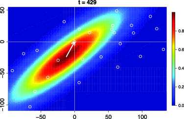
Figure 4: Illustration of the convolution kernel at time $t=429$. The colors indicate the lag-1 influence of the other stations on the station Wynau. The white arrow represents the drift caused by a south-west wind at this time point. The dots represent the observation stations. The axes are in km.

For interpreting the fitted parameters governing the convolution kernel ($\rho_{1}$, $c$, $\alpha$ and $u$), we illustrate in Figure 4 the convolution kernel over the region where the stations lie. The parameters $\rho_{1}$, $c$, $\alpha$ and $u$ are taken at their posterior mode. The plot is interpreted as follows. The height of the kernel is the level of influence that ${\bolds\xi}_{t-1}({\mathbf{s}}^{\prime})$ at location ${\mathbf{s}}^{\prime}$ has on ${\bolds\xi}_{t}({\mathbf{s}})$ at location ${\mathbf{s}}$ as a function of ${\mathbf{s}}^{\prime}-{\mathbf{s}}$. In other words, the colors represent the lag-1 influence of the other stations on the station Wynau which is used as origin in the plot. The white arrow represents the drift vector ${\bolds\mu}_{t}=u\cdot{\mathbf{w}}_{t}$ at time $t=429$, ${\mathbf{w}}_{t}$ being the wind vector. Note that this transport vector changes over time, thus causing temporal nonstationarity. The time $t=429$ illustrates a meteorological situation with the typically predominant southwestern wind direction.

With $c$ and $\alpha$ being approximately $4$ and $0.7$, we observe anisotropy along the south-east north-west direction. This corresponds to the topography of the region, as the area containing a majority of the stations lies between two mountain ranges: the Jura to the north-west and the Alps to the south-east. Correlations are expected to be higher along the flat part between these two mountain ranges.

Furthermore, the plot shows how the external drift shifts the convolution kernel. Apparently, the southwestern neighbor (Bern) has the highest influence on Wynau in this situation, with wind coming from the southwest. Gneiting et al. (2006) observe a similar phenomenon in wind speed data over the U.S. Pacific Northwest where there is also a predominant wind direction causing asymmetric cross-correlations.

4.3 Short term prediction of precipitation

In the following, we apply the fitted models to produce short term predictions of precipitation. As mentioned before, we have fitted the model to the first $720$ time periods from December 2008 to February 2009. From this we obtain posterior distributions for the primary parameters. Predictions for the time periods in March that were set aside are obtained as described in the following.

Ideally, one would run the full MCMC algorithm at each time point, including all data up to the point, and obtain predictive distributions from this. However, since this is rather time consuming, we make the following approximation. We assume that the posterior distribution of the primary parameters given ${\mathbf{Y}}_{1\dvtx t}=\{{\mathbf{Y}}_{1},\ldots,{\mathbf{Y}}_{t}\}$ is the same for all $t\geq 720$. That is, we neglect the additional information that the observations in March give about the primary parameters. In practice, this means that posterior distributions of the primary parameters are calculated only once, namely, on the data set from December 2008 to February 2009.

For each time $t\geq 720$, we make up to $8$ steps ahead forecasts. That is, we sample from the predictive distribution of ${\mathbf{Y}}^{*}_{t+k}$, $k=1,\ldots,8$, given ${\mathbf{Y}}_{1\dvtx t}=\{{\mathbf{Y}}_{1},\ldots,{\mathbf{Y}}_{t}\}$ and given the posterior of the primary parameters based on the data from December 2008 to February 2009. Since the NWP produces forecasts for the three meteorological covariates once a day, for each prediction time $t+k$, the forecasts made at 0:00UTC of the same day are used. Sampling from the predictive distribution consists of imputing the augmented data ${\mathbf{W}}$ and sampling from the latent process ${\bolds\xi}$. These two steps are done as described in Section 3. To generate one sample from the predictive distribution takes around 3.5 seconds on an AMD Athlon(tm) 64 X2 Dual Core Processor 5600$+$ with a 2900 MHz CPU clock rate. We use 200 samples to characterize each predictive distribution.

The assumption that the posterior of the primary parameters does not change may be questionable over longer time periods and when one moves away from the time period from which data is used to obtain the posterior distribution. But since all our data lies in the winter season, we think that this assumption is reasonable. If longer time periods are considered, one could use sliding training windows or model the primary parameters as evolving dynamically over time. One can also investigate how the predictive performance deteriorates with increasing lags between predictions and last time point from which data is used to fit the model.

In addition to the separable model and the nonstationary anisotropic drift model, we fit a model with no autoregressive term, that is, with $\phi=0$. Further, to assess how much information stems from the three meteorological covariates (temperature, dew point and specific humidity) and how much from the dynamic spatio-temporal model, we also fit the nonstationary anisotropic drift model without including these covariates. For each model, we calculate pointwise predictions for the individual stations and also predictions for the areal average. The latter are obtained using the Voronoi tessellation as described in Section 3.2.

In order to asses the performance of the probabilistic predictions, we use the continuous ranked probability score (CRPS) [Matheson and Winkler (1976)]. The CRPS is a strictly proper scoring rule [Gneiting and Raftery (2007)] that assigns a numerical value to probabilistic forecasts and assesses calibration and sharpness simultaneously [Gneiting, Balabdaoui and Raftery (2007)]. It is defined as

$$\operatorname{CRPS}(F,y)=\int_{-\infty}^{\infty}\bigl{(}F(x)-\mathbf{1}_{\{y\leq x\}}\bigr{)}^{2}\,dx,$$ (29)

where $F$ is the predictive cumulative distribution function, $y$ is the observed realization, and $\mathbf{1}$ is an indicator function. It can be equivalently calculated as

$$\operatorname{CRPS}(F,y)=E_{F}|Y-y|-\tfrac{1}{2}E_{F}\bigl{|}Y-Y^{\prime}\bigr{|},$$ (30)

where $Y$ and $Y^{\prime}$ are independent random variables with distribution $F$. If a sample $Y^{(1)},\ldots,Y^{(m)}$ from $F$ is available, it can be approximated by

$$\frac{1}{m}\sum_{i=1}^{m}\bigl{|}Y^{(i)}-y\bigr{|}-\frac{1}{2m^{2}}\sum_{i,j=1}^{m}\bigl{|}Y^{(i)}-Y^{(j)}\bigr{|}.$$ (31)

In Figure 5 the average CRPS of the pointwise predictions and the areal predictions are plotted versus lead times. In the left plot, the mean is taken over all stations and time periods, whereas the areal version is an average over all time periods. Predictions ${\mathbf{Y}}^{*}_{t+k}$, $k=1,\ldots,8$, for the next 8 time steps are made at each time point $t$. We recall that the NWP model produces predictions for 8 consecutive periods once a day at midnight. For simplicity, potential diurnal variation in the accuracy of the predicted covariates is ignored.

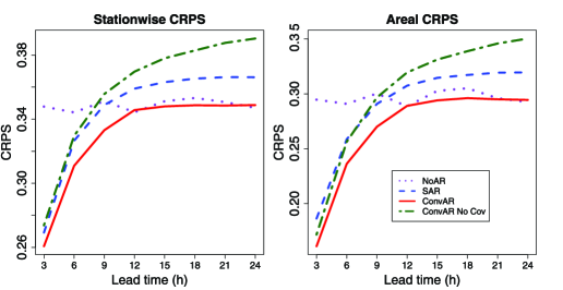
Figure 5: Comparison of statistical models. The continuous ranked probability score (CRPS) of forecasts versus number of consecutive time periods for which predictions are made is shown. On the left are CRPSs of station specific forecasts and on the right are CRPSs of areal forecasts. “NoAR” denotes the model without an autoregressive term, “SAR” the one with a separable covariance structure, and “ConvAR” the convolution based nonstationary anisotropic drift model. All three models include the covariates described in Section 4.1. A convolution based model without including covariates (“ConvAR No Cov”) is also fitted. The unit of the CRPS is mm.

We see that the nonstationary anisotropic drift model (“ConvAR”) has clearly the best performance among the three models. In particular, the nonseparable convolution based model performs better than the simpler separable spatio-temporal model (“SAR”). Not surprisingly, the model without temporal dependency (“NoAR”) performs worse than the other two models. Comparing the “ConvAR” model, the nonstationary convolution model without covariates (“ConvAR No Cov”), and the “NoAR” model, we see that the main source of predictive performance at small lead times is not the covariates but the dynamic spatio-temporal model. In the areal case, the nonstationary convolution model without covariates even outperforms the simple autoregressive model including covariates at small lead times. With increasing lead time, the meteorological covariates contribute more to the predictive performance and the dynamic spatio-temporal model becomes less important.

We also compare the performance of the predictions from the nonstationary anisotropic drift model with predictions obtained from the NWP model. Since the NWP model produces deterministic forecasts, we use the mean absolute error (MAE). In order to make the comparison fair, we first reduce the statistical distributional forecast to a point forecast by taking the median [see Gneiting (2011) on why this is a reasonable choice]. As mentioned, the NWP model produces predictions once a day starting at 0:00UTC. Predictions are then made for eight consecutive time periods corresponding to 24 h ahead. This means that the time of day also corresponds to the lead time. This is in contrast to the above comparison of the different statistical models where 8 step ahead predictions were made at all time periods.

In Figure 6 the mean absolute error (MAE) of forecasts versus lead time, or time of day is

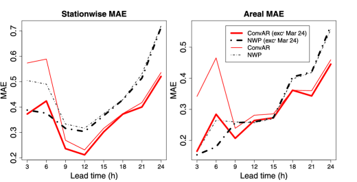
Figure 6: Comparison of statistical and NWP model. The mean absolute error (MAE) of forecasts versus lead time is shown. Lead time also corresponds to the time of day. The left panel shows MAEs of station specific forecasts averaged over time and the stations, and the right panel shows MAEs of areal forecasts averaged over time. “ConvAR” denotes the convolution based nonstationary anisotropic drift model and “NWP” the NWP model. The bold lines show the results when excluding March 24, 2009. The unit of the MAE is mm.

shown. In addition, in Table 2 we report MAEs averaged over all lead times. Note that there is one particular day (March 24) when heavy rainfall occurred shortly after 0:00UTC. We report results including (thin lines) and excluding (bold lines) this day.

Table 2: Comparison of statistical and NWP model. The mean absolute error (MAE) averaged over all days and lead times is reported. “ConvAR” denotes the convolution based nonstationary anisotropic drift model and“NWP” the NWP model. The unit of the MAE is mm

	ConvAR	NWP	Areal ConvAR	Areal NWP
March 2009	0.41	0.46	0.35	0.32
Excluding March 24	0.36	0.43	0.29	0.31

Table 2 shows that overall the statistical model outperforms the NWP on a stationwise base. When considering the areal average, the two models perform similarly. Depending on whether March 24 is included or not, the NWP or the statistical model has a slightly lower average MAE.

Furthermore, Figure 6 shows that March 24 considerably affects the performance of the one- and two-step ahead predictions of the statistical model as well as the stationwise performance of the NWP model. When excluding this day, the corresponding MAEs are considerably lower. This shows a typical behavior of our model and statistical models in general: they perform well when, at the time of prediction, the major phenomena (advective fronts) are already observable. In this case, the spatio-temporal statistical model can extrapolate the space–time dynamics of the rainfall process into the future.

Earlier studies have shown that nowcasting methods, including statistical approaches, perform usually better at short lead times (up to one day), while NWP have higher predictive skills at medium ranges [see Kober et al. (2012) or Little, McSharry and Taylor (2009)]. Our results are in line with these findings in the sense that all lead times used in our application are still in the range of what is considered “short” lead times. However, our model is not just based on past precipitation observations but also on other predicted meteorological variables.

5 Conclusions

A hierarchical Bayesian spatio-temporal model is presented. Incorporating physical knowledge, the dynamic model is nonstationary, anisotropic, and allows for nonseparable covariance structures. It incorporates a drift term that depends on a wind vector. At the data stage, the model determines the probability of rainfall and the rainfall amount distribution together. The model is fitted using Markov chain Monte Carlo (MCMC) methods and applied to obtain short term precipitation forecasts. It performs better than a separable, stationary and isotropic model, and it performs comparably to a deterministic numerical weather prediction model and has the advantage that it quantifies prediction uncertainty.

Even though we have applied the model to prediction of precipitation, it can also be used to predict or interpolate other meteorological quantities of interest.

Future research could focus on adapting the model so that in can be applied to spatially highly resolved data. Using Markov random fields [Rue and Held (2005), Lindgren, Rue and Lindström (2011)] for the innovation process ${\bolds\varepsilon}_{t}$ might be a potential direction. Alternatively, a dimension reduction approach could be examined; cf. Banerjee et al. (2008). For instance, Sigrist, Künsch and Stahel (2012) approximate an advection-diffusion SPDE to cope with large data sets. Further, the model can be extended by additionally relaxing some assumptions. For instance, the parameters $\sigma^{2}$, $\phi$, $\rho_{0}$, $\rho_{1}$ and $\lambda$ were assumed to be constant over time. Assuming periodicity, Fourier harmonics could be used to model parameters that vary seasonally during the year. Alternatively, the parameters could evolve dynamically over time according to an equation of the form $\vartheta_{t}=\vartheta_{t-1}+N(0,\sigma^{2}_{\vartheta})$.

References

- Ailliot, Thompson and Thomson (2009) {barticle}[mr] \bauthor\bsnmAilliot, \bfnmPierre\binitsP., \bauthor\bsnmThompson, \bfnmCraig\binitsC. and \bauthor\bsnmThomson, \bfnmPeter\binitsP. (\byear2009). \btitleSpace–time modelling of precipitation by using a hidden Markov model and censored Gaussian distributions. \bjournalJ. R. Stat. Soc. Ser. C. Appl. Stat. \bvolume58 \bpages405–426. \biddoi=10.1111/j.1467-9876.2008.00654.x, issn=0035-9254, mr=2750013 \bptokimsref \endbibitem
- Allcroft and Glasbey (2003) {barticle}[mr] \bauthor\bsnmAllcroft, \bfnmDavid J.\binitsD. J. and \bauthor\bsnmGlasbey, \bfnmChris A.\binitsC. A. (\byear2003). \btitleA latent Gaussian Markov random-field model for spatiotemporal rainfall disaggregation. \bjournalJ. R. Stat. Soc. Ser. C. Appl. Stat. \bvolume52 \bpages487–498. \biddoi=10.1111/1467-9876.00419, issn=0035-9254, mr=2012972 \bptokimsref \endbibitem
- Banerjee et al. (2008) {barticle}[mr] \bauthor\bsnmBanerjee, \bfnmSudipto\binitsS., \bauthor\bsnmGelfand, \bfnmAlan E.\binitsA. E., \bauthor\bsnmFinley, \bfnmAndrew O.\binitsA. O. and \bauthor\bsnmSang, \bfnmHuiyan\binitsH. (\byear2008). \btitleGaussian predictive process models for large spatial data sets. \bjournalJ. R. Stat. Soc. Ser. B Stat. Methodol. \bvolume70 \bpages825–848. \biddoi=10.1111/j.1467-9868.2008.00663.x, issn=1369-7412, mr=2523906 \bptokimsref \endbibitem
- Bardossy and Plate (1992) {barticle}[author] \bauthor\bsnmBardossy, \bfnmA.\binitsA. and \bauthor\bsnmPlate, \bfnmE. J.\binitsE. J. (\byear1992). \btitleSpace–time model for daily rainfall using atmospheric circulation patterns. \bjournalWater Resources Research \bvolume28 \bpages1247–1259. \bptokimsref \endbibitem
- Bell (1987) {barticle}[author] \bauthor\bsnmBell, \bfnmTL\binitsT. (\byear1987). \btitleA space–time stochastic model of rainfall for satellite remote-sensing studies. \bjournalJournal of Geophysical Research \bvolume92 \bpages9631–9643. \bptokimsref \endbibitem
- Bellone, Hughes and Guttorp (2000) {barticle}[author] \bauthor\bsnmBellone, \bfnmE.\binitsE., \bauthor\bsnmHughes, \bfnmJ. P.\binitsJ. P. and \bauthor\bsnmGuttorp, \bfnmP.\binitsP. (\byear2000). \btitleA hidden Markov model for downscaling synoptic atmospheric patterns to precipitation amounts. \bjournalClimate Research \bvolume15 \bpages1–12. \bptokimsref \endbibitem
- Berger, De Oliveira and Sansó (2001) {barticle}[mr] \bauthor\bsnmBerger, \bfnmJames O.\binitsJ. O., \bauthor\bsnmDe Oliveira, \bfnmVictor\binitsV. and \bauthor\bsnmSansó, \bfnmBruno\binitsB. (\byear2001). \btitleObjective Bayesian analysis of spatially correlated data. \bjournalJ. Amer. Statist. Assoc. \bvolume96 \bpages1361–1374. \biddoi=10.1198/016214501753382282, issn=0162-1459, mr=1946582 \bptokimsref \endbibitem
- Berrocal, Raftery and Gneiting (2008) {barticle}[mr] \bauthor\bsnmBerrocal, \bfnmVeronica J.\binitsV. J., \bauthor\bsnmRaftery, \bfnmAdrian E.\binitsA. E. and \bauthor\bsnmGneiting, \bfnmTilmann\binitsT. (\byear2008). \btitleProbabilistic quantitative precipitation field forecasting using a two-stage spatial model. \bjournalAnn. Appl. Stat. \bvolume2 \bpages1170–1193. \biddoi=10.1214/08-AOAS203, issn=1932-6157, mr=2655654 \bptokimsref \endbibitem
- Brown et al. (2000) {barticle}[mr] \bauthor\bsnmBrown, \bfnmPatrick E.\binitsP. E., \bauthor\bsnmKåresen, \bfnmKjetil F.\binitsK. F., \bauthor\bsnmRoberts, \bfnmGareth O.\binitsG. O. and \bauthor\bsnmTonellato, \bfnmStefano\binitsS. (\byear2000). \btitleBlur-generated non-separable space–time models. \bjournalJ. R. Stat. Soc. Ser. B Stat. Methodol. \bvolume62 \bpages847–860. \biddoi=10.1111/1467-9868.00269, issn=1369-7412, mr=1796297 \bptokimsref \endbibitem
- Brown et al. (2001) {barticle}[mr] \bauthor\bsnmBrown, \bfnmPatrick E.\binitsP. E., \bauthor\bsnmDiggle, \bfnmPeter J.\binitsP. J., \bauthor\bsnmLord, \bfnmMartin E.\binitsM. E. and \bauthor\bsnmYoung, \bfnmPeter C.\binitsP. C. (\byear2001). \btitleSpace–time calibration of radar rainfall data. \bjournalJ. R. Stat. Soc. Ser. C. Appl. Stat. \bvolume50 \bpages221–241. \biddoi=10.1111/1467-9876.00230, issn=0035-9254, mr=1833274 \bptokimsref \endbibitem
- Carter and Kohn (1994) {barticle}[mr] \bauthor\bsnmCarter, \bfnmC. K.\binitsC. K. and \bauthor\bsnmKohn, \bfnmR.\binitsR. (\byear1994). \btitleOn Gibbs sampling for state space models. \bjournalBiometrika \bvolume81 \bpages541–553. \biddoi=10.1093/biomet/81.3.541, issn=0006-3444, mr=1311096 \bptokimsref \endbibitem
- Charles, Bates and Hughes (1999) {barticle}[author] \bauthor\bsnmCharles, \bfnmSP\binitsS., \bauthor\bsnmBates, \bfnmBC\binitsB. and \bauthor\bsnmHughes, \bfnmJP\binitsJ. (\byear1999). \btitleA spatiotemporal model for downscaling precipitation occurrence and amounts. \bjournalJournal of Geophysical Research \bvolume104 \bpages31657–31669. \bptokimsref \endbibitem
- Chib and Greenberg (1995) {barticle}[author] \bauthor\bsnmChib, \bfnmSiddhartha\binitsS. and \bauthor\bsnmGreenberg, \bfnmEdward\binitsE. (\byear1995). \btitleUnderstanding the Metropolis–Hastings algorithm. \bjournalAmer. Statist. \bvolume49 \bpages327–335. \bptokimsref \endbibitem
- Coe and Stern (1982) {barticle}[author] \bauthor\bsnmCoe, \bfnmR.\binitsR. and \bauthor\bsnmStern, \bfnmRD\binitsR. (\byear1982). \btitleFitting models to daily rainfall data. \bjournalJournal of Applied Meteorology \bvolume21 \bpages1024–1031. \bptokimsref \endbibitem
- Cox and Isham (1988) {barticle}[mr] \bauthor\bsnmCox, \bfnmD. R.\binitsD. R. and \bauthor\bsnmIsham, \bfnmValerie\binitsV. (\byear1988). \btitleA simple spatial–temporal model of rainfall. \bjournalProc. R. Soc. Lond. Ser. A Math. Phys. Eng. Sci. \bvolume415 \bpages317–328. \bidissn=0962-8444, mr=0932924 \bptokimsref \endbibitem
- Cressie (1993) {bbook}[mr] \bauthor\bsnmCressie, \bfnmNoel A. C.\binitsN. A. C. (\byear1993). \btitleStatistics for Spatial Data, \bedition2nd ed. \bpublisherWiley, \baddressNew York. \bptokimsref \endbibitem
- Cressie and Huang (1999) {barticle}[mr] \bauthor\bsnmCressie, \bfnmNoel\binitsN. and \bauthor\bsnmHuang, \bfnmHsin-Cheng\binitsH.-C. (\byear1999). \btitleClasses of nonseparable, spatio-temporal stationary covariance functions. \bjournalJ. Amer. Statist. Assoc. \bvolume94 \bpages1330–1340. \biddoi=10.2307/2669946, issn=0162-1459, mr=1731494 \bptokimsref \endbibitem
- Cressie and Wikle (2011) {bbook}[mr] \bauthor\bsnmCressie, \bfnmNoel\binitsN. and \bauthor\bsnmWikle, \bfnmChristopher K.\binitsC. K. (\byear2011). \btitleStatistics for Spatio-Temporal Data. \bpublisherWiley, \baddressHoboken, NJ. \bidmr=2848400 \bptokimsref \endbibitem
- Diggle, Tawn and Moyeed (1998) {barticle}[mr] \bauthor\bsnmDiggle, \bfnmP. J.\binitsP. J., \bauthor\bsnmTawn, \bfnmJ. A.\binitsJ. A. and \bauthor\bsnmMoyeed, \bfnmR. A.\binitsR. A. (\byear1998). \btitleModel-based geostatistics. \bjournalJ. R. Stat. Soc. Ser. C. Appl. Stat. \bvolume47 \bpages299–350. \bnoteWith discussion and a reply by the authors. \biddoi=10.1111/1467-9876.00113, issn=0035-9254, mr=1626544 \bptnotecheck related\bptokimsref \endbibitem
- Fowler et al. (2005) {barticle}[author] \bauthor\bsnmFowler, \bfnmH. J.\binitsH. J., \bauthor\bsnmKilsby, \bfnmC. G.\binitsC. G., \bauthor\bsnmO’Connell, \bfnmP. E.\binitsP. E. and \bauthor\bsnmBurton, \bfnmA.\binitsA. (\byear2005). \btitleA weather-type conditioned multi-site stochastic rainfall model for the generation of scenarios of climatic variability and change. \bjournalJournal of Hydrology \bvolume308 \bpages50–66. \bptokimsref \endbibitem
- Frühwirth-Schnatter (1994) {barticle}[mr] \bauthor\bsnmFrühwirth-Schnatter, \bfnmSylvia\binitsS. (\byear1994). \btitleData augmentation and dynamic linear models. \bjournalJ. Time Series Anal. \bvolume15 \bpages183–202. \biddoi=10.1111/j.1467-9892.1994.tb00184.x, issn=0143-9782, mr=1263889 \bptokimsref \endbibitem
- Fuentes, Reich and Lee (2008) {barticle}[mr] \bauthor\bsnmFuentes, \bfnmMontserrat\binitsM., \bauthor\bsnmReich, \bfnmBrian\binitsB. and \bauthor\bsnmLee, \bfnmGyuwon\binitsG. (\byear2008). \btitleSpatial–temporal mesoscale modeling of rainfall intensity using gage and radar data. \bjournalAnn. Appl. Stat. \bvolume2 \bpages1148–1169. \biddoi=10.1214/08-AOAS166, issn=1932-6157, mr=2655653 \bptokimsref \endbibitem
- Gelfand, Banerjee and Gamerman (2005) {barticle}[mr] \bauthor\bsnmGelfand, \bfnmAlan E.\binitsA. E., \bauthor\bsnmBanerjee, \bfnmSudipto\binitsS. and \bauthor\bsnmGamerman, \bfnmDani\binitsD. (\byear2005). \btitleSpatial process modelling for univariate and multivariate dynamic spatial data. \bjournalEnvironmetrics \bvolume16 \bpages465–479. \biddoi=10.1002/env.715, issn=1180-4009, mr=2147537 \bptokimsref \endbibitem
- Gelfand and Smith (1990) {barticle}[mr] \bauthor\bsnmGelfand, \bfnmAlan E.\binitsA. E. and \bauthor\bsnmSmith, \bfnmAdrian F. M.\binitsA. F. M. (\byear1990). \btitleSampling-based approaches to calculating marginal densities. \bjournalJ. Amer. Statist. Assoc. \bvolume85 \bpages398–409. \bidissn=0162-1459, mr=1141740 \bptokimsref \endbibitem
- Gelfand et al. (2010) {bbook}[mr] \beditor\bsnmGelfand, \bfnmAlan E.\binitsA. E., \beditor\bsnmDiggle, \bfnmPeter J.\binitsP. J., \beditor\bsnmFuentes, \bfnmMontserrat\binitsM. and \beditor\bsnmGuttorp, \bfnmPeter\binitsP., eds. (\byear2010). \btitleHandbook of Spatial Statistics. \bpublisherCRC Press, \baddressBoca Raton, FL. \biddoi=10.1201/9781420072884, mr=2761512 \bptokimsref \endbibitem
- Gneiting (2002) {barticle}[mr] \bauthor\bsnmGneiting, \bfnmTilmann\binitsT. (\byear2002). \btitleNonseparable, stationary covariance functions for space–time data. \bjournalJ. Amer. Statist. Assoc. \bvolume97 \bpages590–600. \biddoi=10.1198/016214502760047113, issn=0162-1459, mr=1941475 \bptokimsref \endbibitem
- Gneiting (2011) {barticle}[mr] \bauthor\bsnmGneiting, \bfnmTilmann\binitsT. (\byear2011). \btitleMaking and evaluating point forecasts. \bjournalJ. Amer. Statist. Assoc. \bvolume106 \bpages746–762. \biddoi=10.1198/jasa.2011.r10138, issn=0162-1459, mr=2847988 \bptokimsref \endbibitem
- Gneiting, Balabdaoui and Raftery (2007) {barticle}[mr] \bauthor\bsnmGneiting, \bfnmTilmann\binitsT., \bauthor\bsnmBalabdaoui, \bfnmFadoua\binitsF. and \bauthor\bsnmRaftery, \bfnmAdrian E.\binitsA. E. (\byear2007). \btitleProbabilistic forecasts, calibration and sharpness. \bjournalJ. R. Stat. Soc. Ser. B Stat. Methodol. \bvolume69 \bpages243–268. \biddoi=10.1111/j.1467-9868.2007.00587.x, issn=1369-7412, mr=2325275 \bptokimsref \endbibitem
- Gneiting, Genton and Guttorp (2007) {bincollection}[author] \bauthor\bsnmGneiting, \bfnmTilmann\binitsT., \bauthor\bsnmGenton, \bfnmMarc G.\binitsM. G. and \bauthor\bsnmGuttorp, \bfnmPeter\binitsP. (\byear2007). \btitleGeostatistical space–time models, stationarity, separability and full symmetry. In \bbooktitleStatistical Methods for Spatio-Temporal Systems (\beditor\bfnmB.\binitsB. \bsnmFinkenstädt, \beditor\bfnmL.\binitsL. \bsnmHeld and \beditor\bfnmV.\binitsV. \bsnmIsham, eds.). \bseriesMonographs on Statistics and Applied Probability \bvolume107 \bpages151–175. \bpublisherChapman & Hall/CRC, \baddressBoca Raton. \bptokimsref \endbibitem
- Gneiting and Raftery (2007) {barticle}[mr] \bauthor\bsnmGneiting, \bfnmTilmann\binitsT. and \bauthor\bsnmRaftery, \bfnmAdrian E.\binitsA. E. (\byear2007). \btitleStrictly proper scoring rules, prediction, and estimation. \bjournalJ. Amer. Statist. Assoc. \bvolume102 \bpages359–378. \biddoi=10.1198/016214506000001437, issn=0162-1459, mr=2345548 \bptokimsref \endbibitem
- Gneiting et al. (2006) {barticle}[mr] \bauthor\bsnmGneiting, \bfnmTilmann\binitsT., \bauthor\bsnmLarson, \bfnmKristin\binitsK., \bauthor\bsnmWestrick, \bfnmKenneth\binitsK., \bauthor\bsnmGenton, \bfnmMarc G.\binitsM. G. and \bauthor\bsnmAldrich, \bfnmEric\binitsE. (\byear2006). \btitleCalibrated probabilistic forecasting at the stateline wind energy center: The regime-switching space–time method. \bjournalJ. Amer. Statist. Assoc. \bvolume101 \bpages968–979. \biddoi=10.1198/016214506000000456, issn=0162-1459, mr=2324108 \bptokimsref \endbibitem
- Hastings (1970) {barticle}[author] \bauthor\bsnmHastings, \bfnmW. K.\binitsW. K. (\byear1970). \btitleMonte Carlo sampling methods using Markov chains and their applications. \bjournalBiometrika \bvolume57 \bpages97–109. \bptokimsref \endbibitem
- Hernández, Guenni and Sansó (2009) {barticle}[mr] \bauthor\bsnmHernández, \bfnmAracelis\binitsA., \bauthor\bsnmGuenni, \bfnmLelys\binitsL. and \bauthor\bsnmSansó, \bfnmBruno\binitsB. (\byear2009). \btitleExtreme limit distribution of truncated models for daily rainfall. \bjournalEnvironmetrics \bvolume20 \bpages962–980. \biddoi=10.1002/env.967, issn=1180-4009, mr=2838498 \bptokimsref \endbibitem
- Huang and Hsu (2004) {barticle}[author] \bauthor\bsnmHuang, \bfnmHsin-Cheng\binitsH.-C. and \bauthor\bsnmHsu, \bfnmNan-Jung\binitsN.-J. (\byear2004). \btitleModeling transport effects on ground-level ozone using a non-stationary space–time model. \bjournalEnvironmetrics \bvolume15 \bpages251–268. \bptokimsref \endbibitem
- Hughes and Guttorp (1994) {barticle}[author] \bauthor\bsnmHughes, \bfnmJP\binitsJ. and \bauthor\bsnmGuttorp, \bfnmP.\binitsP. (\byear1994). \btitleA class of stochastic models for relating synoptic atmospheric patterns to regional hydrologic phenomena. \bjournalWater Resources Research \bvolume30 \bpages1535–1546. \bptokimsref \endbibitem
- Hughes, Guttorp and Charles (1999) {barticle}[author] \bauthor\bsnmHughes, \bfnmJP\binitsJ., \bauthor\bsnmGuttorp, \bfnmP.\binitsP. and \bauthor\bsnmCharles, \bfnmS. P.\binitsS. P. (\byear1999). \btitleA non-homogeneous hidden Markov model for precipitation occurrence. \bjournalJ. R. Stat. Soc. Ser. C. Appl. Stat. \bvolume48 \bpages15–30. \bptokimsref \endbibitem
- Hutchinson (1995) {barticle}[author] \bauthor\bsnmHutchinson, \bfnmMF\binitsM. (\byear1995). \btitleStochastic space–time weather models from ground-based data. \bjournalAgricultural and Forest Meteorology \bvolume73 \bpages237–264. \bptokimsref \endbibitem
- Isham and Cox (1994) {binproceedings}[author] \bauthor\bsnmIsham, \bfnmValerie\binitsV. and \bauthor\bsnmCox, \bfnmDavid Roxbee\binitsD. R. (\byear1994). \btitleStochastic models of precipitation. In \bbooktitleStatistics for the Environment, Vol. 2 (\beditor\bfnmVic\binitsV. \bsnmBarnett and \beditor\bfnmK. Feridun\binitsK. F. \bsnmTurkmann, eds.). \bpublisherWiley, \baddressChichester. \bptokimsref \endbibitem
- Jones and Zhang (1997) {bincollection}[author] \bauthor\bsnmJones, \bfnmR. H.\binitsR. H. and \bauthor\bsnmZhang, \bfnmY.\binitsY. (\byear1997). \btitleModels for continuous stationary space–time processes. In \bbooktitleStatistical Methods for Spatio-Temporal Systems (\beditor\bfnmT. G.\binitsT. G. \bsnmGregoire, \beditor\bfnmD. R.\binitsD. R. \bsnmBrillinger, \beditor\bfnmP. J.\binitsP. J. \bsnmDiggle, \beditor\bfnmE.\binitsE. \bsnmRussek-Cohen, \beditor\bfnmW. G.\binitsW. G. \bsnmWarren and \beditor\bfnmR. D.\binitsR. D. \bsnmWolfinger, eds.). \bseriesLecture Notes in Statistics \bvolume122 \bpages289–298. \bpublisherSpringer, \baddressNew York. \bptokimsref \endbibitem
- Kober et al. (2012) {barticle}[author] \bauthor\bsnmKober, \bfnmK.\binitsK., \bauthor\bsnmCraig, \bfnmG. C.\binitsG. C., \bauthor\bsnmKeil, \bfnmC.\binitsC. and \bauthor\bsnmDörnbrack, \bfnmA.\binitsA. (\byear2012). \btitleBlending a probabilistic nowcasting method with a high-resolution numerical weather prediction ensemble for convective precipitation forecasts. \bjournalQuarterly Journal of the Royal Meteorological Society \bvolume138 \bpages755–768. \bptokimsref \endbibitem
- Künsch (2001) {bincollection}[mr] \bauthor\bsnmKünsch, \bfnmHans R.\binitsH. R. (\byear2001). \btitleState space and hidden Markov models. In \bbooktitleComplex Stochastic Systems (Eindhoven, 1999). \bseriesMonographs on Statistics and Applied Probability \bvolume87 \bpages109–173. \bpublisherChapman & Hall/CRC, \baddressBoca Raton, FL. \bidmr=1893412 \bptokimsref \endbibitem
- Kyriakidis and Journel (1999) {barticle}[mr] \bauthor\bsnmKyriakidis, \bfnmPhaedon C.\binitsP. C. and \bauthor\bsnmJournel, \bfnmAndré G.\binitsA. G. (\byear1999). \btitleGeostatistical space–time models: A review. \bjournalMath. Geol. \bvolume31 \bpages651–684. \biddoi=10.1023/A:1007528426688, issn=0882-8121, mr=1694654 \bptokimsref \endbibitem
- Le Cam (1961) {bincollection}[mr] \bauthor\bsnmLe Cam, \bfnmL.\binitsL. (\byear1961). \btitleA stochastic description of precipitation. In \bbooktitleProc. 4th Berkeley Sympos. Math. Statist. and Prob., Vol. III \bpages165–186. \bpublisherUniv. California Press, \baddressBerkeley, CA. \bidmr=0135598 \bptokimsref \endbibitem
- Lindgren, Rue and Lindström (2011) {barticle}[mr] \bauthor\bsnmLindgren, \bfnmFinn\binitsF., \bauthor\bsnmRue, \bfnmHåvard\binitsH. and \bauthor\bsnmLindström, \bfnmJohan\binitsJ. (\byear2011). \btitleAn explicit link between Gaussian fields and Gaussian Markov random fields: The stochastic partial differential equation approach. \bjournalJ. R. Stat. Soc. Ser. B Stat. Methodol. \bvolume73 \bpages423–498. \bnoteWith discussion and a reply by the authors. \biddoi=10.1111/j.1467-9868.2011.00777.x, issn=1369-7412, mr=2853727 \bptnotecheck related\bptokimsref \endbibitem
- Little, McSharry and Taylor (2009) {barticle}[author] \bauthor\bsnmLittle, \bfnmM. A.\binitsM. A., \bauthor\bsnmMcSharry, \bfnmP. E.\binitsP. E. and \bauthor\bsnmTaylor, \bfnmJ. W.\binitsJ. W. (\byear2009). \btitleGeneralized linear models for site-specific density forecasting of U.K. daily rainfall. \bjournalMonthly Weather Review \bvolume137 \bpages1029–1045. \bptokimsref \endbibitem
- Ma (2003) {barticle}[mr] \bauthor\bsnmMa, \bfnmChunsheng\binitsC. (\byear2003). \btitleFamilies of spatio-temporal stationary covariance models. \bjournalJ. Statist. Plann. Inference \bvolume116 \bpages489–501. \biddoi=10.1016/S0378-3758(02)00353-1, issn=0378-3758, mr=2000096 \bptokimsref \endbibitem
- Makhnin and McAllister (2009) {barticle}[author] \bauthor\bsnmMakhnin, \bfnmOleg V.\binitsO. V. and \bauthor\bsnmMcAllister, \bfnmDevon L.\binitsD. L. (\byear2009). \btitleStochastic precipitation generation based on a multivariate autoregression model. \bjournalJournal of Hydrometeorology \bvolume10 \bpages1397–1413. \bptokimsref \endbibitem
- Mardia and Watkins (1989) {barticle}[mr] \bauthor\bsnmMardia, \bfnmK. V.\binitsK. V. and \bauthor\bsnmWatkins, \bfnmA. J.\binitsA. J. (\byear1989). \btitleOn multimodality of the likelihood in the spatial linear model. \bjournalBiometrika \bvolume76 \bpages289–295. \biddoi=10.1093/biomet/76.2.289, issn=0006-3444, mr=1016019 \bptokimsref \endbibitem
- Mason (1986) {barticle}[author] \bauthor\bsnmMason, \bfnmJohn\binitsJ. (\byear1986). \btitleNumerical weather prediction. \bjournalProc. R. Soc. Lond. Ser. A Math. Phys. Eng. Sci. \bvolume407 \bpages51–60. \bptokimsref \endbibitem
- Matheson and Winkler (1976) {barticle}[author] \bauthor\bsnmMatheson, \bfnmJames E.\binitsJ. E. and \bauthor\bsnmWinkler, \bfnmRobert L.\binitsR. L. (\byear1976). \btitleScoring rules for continuous probability distributions. \bjournalManag. Sci. \bvolume22 \bpages1087–1096. \bptokimsref \endbibitem
- Metropolis et al. (1953) {barticle}[author] \bauthor\bsnmMetropolis, \bfnmNicholas\binitsN., \bauthor\bsnmRosenbluth, \bfnmArianna W.\binitsA. W., \bauthor\bsnmRosenbluth, \bfnmMarshall N.\binitsM. N., \bauthor\bsnmTeller, \bfnmAugusta H.\binitsA. H. and \bauthor\bsnmTeller, \bfnmEdward\binitsE. (\byear1953). \btitleEquation of state calculations by fast computing machines. \bjournalJ. Chem. Phys. \bvolume21 \bpages1087–1092. \bptokimsref \endbibitem
- Okabe et al. (2000) {bbook}[mr] \bauthor\bsnmOkabe, \bfnmAtsuyuki\binitsA., \bauthor\bsnmBoots, \bfnmBarry\binitsB., \bauthor\bsnmSugihara, \bfnmKokichi\binitsK. and \bauthor\bsnmChiu, \bfnmSung Nok\binitsS. N. (\byear2000). \btitleSpatial Tessellations: Concepts and Applications of Voronoi Diagrams, \bedition2nd ed. \bpublisherWiley, \baddressChichester. \bidmr=1770006 \bptokimsref \endbibitem
- Paciorek and Schervish (2006) {barticle}[mr] \bauthor\bsnmPaciorek, \bfnmChristopher J.\binitsC. J. and \bauthor\bsnmSchervish, \bfnmMark J.\binitsM. J. (\byear2006). \btitleSpatial modelling using a new class of nonstationary covariance functions. \bjournalEnvironmetrics \bvolume17 \bpages483–506. \biddoi=10.1002/env.785, issn=1180-4009, mr=2240939 \bptokimsref \endbibitem
- Rue and Held (2005) {bbook}[mr] \bauthor\bsnmRue, \bfnmHåvard\binitsH. and \bauthor\bsnmHeld, \bfnmLeonhard\binitsL. (\byear2005). \btitleGaussian Markov Random Fields: Theory and Applications. \bseriesMonographs on Statistics and Applied Probability \bvolume104. \bpublisherChapman & Hall/CRC, \baddressBoca Raton, FL. \biddoi=10.1201/9780203492024, mr=2130347 \bptokimsref \endbibitem
- Sansó and Guenni (1999a) {barticle}[author] \bauthor\bsnmSansó, \bfnmB.\binitsB. and \bauthor\bsnmGuenni, \bfnmL.\binitsL. (\byear1999a). \btitleVenezuelan rainfall data analysed by using a Bayesian space–time model. \bjournalJ. R. Stat. Soc. Ser. C. Appl. Stat. \bvolume48 \bpages345–362. \bptokimsref \endbibitem
- Sansó and Guenni (1999b) {barticle}[author] \bauthor\bsnmSansó, \bfnmB.\binitsB. and \bauthor\bsnmGuenni, \bfnmL.\binitsL. (\byear1999b). \btitleA stochastic model for tropical rainfall at a single location. \bjournalJournal of Hydrology \bvolume214 \bpages64–73. \bptokimsref \endbibitem
- Sansó and Guenni (2000) {barticle}[mr] \bauthor\bsnmSansó, \bfnmBruno\binitsB. and \bauthor\bsnmGuenni, \bfnmLelys\binitsL. (\byear2000). \btitleA nonstationary multisite model for rainfall. \bjournalJ. Amer. Statist. Assoc. \bvolume95 \bpages1089–1100. \biddoi=10.2307/2669745, issn=0162-1459, mr=1821717 \bptokimsref \endbibitem
- Sansó and Guenni (2004) {barticle}[author] \bauthor\bsnmSansó, \bfnmB.\binitsB. and \bauthor\bsnmGuenni, \bfnmL.\binitsL. (\byear2004). \btitleA Bayesian approach to compare observed rainfall data to deterministic simulations. \bjournalEnvironmetrics \bvolume15 \bpages597–612. \bptokimsref \endbibitem
- Sigrist, Künsch and Stahel (2012) {bmisc}[author] \bauthor\bsnmSigrist, \bfnmF.\binitsF., \bauthor\bsnmKünsch, \bfnmH. R.\binitsH. R. and \bauthor\bsnmStahel, \bfnmW. A.\binitsW. A. (\byear2012). \bhowpublishedAn SPDE based spatio-temporal model for large data sets with an application to postprocessing precipitation forecasts. Preprint. Available at http://arxiv.org/abs/1204.6118. \bptokimsref \endbibitem
- Sloughter et al. (2007) {barticle}[author] \bauthor\bsnmSloughter, \bfnmJ. McLean\binitsJ. M., \bauthor\bsnmRaftery, \bfnmAdrian E.\binitsA. E., \bauthor\bsnmGneiting, \bfnmTilmann\binitsT. and \bauthor\bsnmFraley, \bfnmChris\binitsC. (\byear2007). \btitleProbabilistic quantitative precipitation forecasting using Bayesian model averaging. \bjournalMonthly Weather Review \bvolume135 \bpages3209–3220. \bptokimsref \endbibitem
- Smith and Roberts (1993) {barticle}[mr] \bauthor\bsnmSmith, \bfnmA. F. M.\binitsA. F. M. and \bauthor\bsnmRoberts, \bfnmG. O.\binitsG. O. (\byear1993). \btitleBayesian computation via the Gibbs sampler and related Markov chain Monte Carlo methods. \bjournalJ. R. Stat. Soc. Ser. B Stat. Methodol. \bvolume55 \bpages3–23. \bidissn=0035-9246, mr=1210421 \bptokimsref \endbibitem
- Sølna and Switzer (1996) {barticle}[mr] \bauthor\bsnmSølna, \bfnmKnut\binitsK. and \bauthor\bsnmSwitzer, \bfnmPaul\binitsP. (\byear1996). \btitleTime trend estimation for a geographic region. \bjournalJ. Amer. Statist. Assoc. \bvolume91 \bpages577–589. \biddoi=10.2307/2291654, issn=0162-1459, mr=1395727 \bptokimsref \endbibitem
- Stehlik and Bardossy (2002) {barticle}[author] \bauthor\bsnmStehlik, \bfnmJ.\binitsJ. and \bauthor\bsnmBardossy, \bfnmA.\binitsA. (\byear2002). \btitleMultivariate stochastic downscaling model for generating daily precipitation series based on atmospheric circulation. \bjournalJournal of Hydrology \bvolume256 \bpages120–141. \bptokimsref \endbibitem
- Stein (1990) {barticle}[mr] \bauthor\bsnmStein, \bfnmMichael\binitsM. (\byear1990). \btitleUniform asymptotic optimality of linear predictions of a random field using an incorrect second-order structure. \bjournalAnn. Statist. \bvolume18 \bpages850–872. \biddoi=10.1214/aos/1176347629, issn=0090-5364, mr=1056340 \bptokimsref \endbibitem
- Stein (2005) {barticle}[mr] \bauthor\bsnmStein, \bfnmMichael L.\binitsM. L. (\byear2005). \btitleSpace–time covariance functions. \bjournalJ. Amer. Statist. Assoc. \bvolume100 \bpages310–321. \biddoi=10.1198/016214504000000854, issn=0162-1459, mr=2156840 \bptokimsref \endbibitem
- Stern and Coe (1984) {barticle}[author] \bauthor\bsnmStern, \bfnmR. D.\binitsR. D. and \bauthor\bsnmCoe, \bfnmR.\binitsR. (\byear1984). \btitleA model fitting analysis of daily rainfall data. \bjournalJ. Roy. Statist. Soc. Ser. A \bvolume147 \bpages1–34. \bptokimsref \endbibitem
- Stidd (1973) {barticle}[author] \bauthor\bsnmStidd, \bfnmC. K.\binitsC. K. (\byear1973). \btitleEstimating the precipitation climate. \bjournalWater Resources Research \bvolume9 \bpages1235–1241. \bptokimsref \endbibitem
- Tobin (1958) {barticle}[mr] \bauthor\bsnmTobin, \bfnmJames\binitsJ. (\byear1958). \btitleEstimation of relationships for limited dependent variables. \bjournalEconometrica \bvolume26 \bpages24–36. \bidissn=0012-9682, mr=0090462 \bptokimsref \endbibitem
- Voronoi (1908) {barticle}[author] \bauthor\bsnmVoronoi, \bfnmGeorges\binitsG. (\byear1908). \btitleNouvelles applications des paramètres continus à la théorie des formes quadratiques. Deuxième mémoire. Recherches sur les parallélloèdres primitifs. \bjournalJournal Für die Reine und Angewandte Mathematik (Crelles Journal) \bvolume1908 \bpages198–287. \bptokimsref \endbibitem
- Warnes and Ripley (1987) {barticle}[mr] \bauthor\bsnmWarnes, \bfnmJ. J.\binitsJ. J. and \bauthor\bsnmRipley, \bfnmB. D.\binitsB. D. (\byear1987). \btitleProblems with likelihood estimation of covariance functions of spatial Gaussian processes. \bjournalBiometrika \bvolume74 \bpages640–642. \biddoi=10.1093/biomet/74.3.640, issn=0006-3444, mr=0909370 \bptokimsref \endbibitem
- Waymire, Gupta and Rodriguez-Iturbe (1984) {barticle}[author] \bauthor\bsnmWaymire, \bfnmE.\binitsE., \bauthor\bsnmGupta, \bfnmV. K.\binitsV. K. and \bauthor\bsnmRodriguez-Iturbe, \bfnmI.\binitsI. (\byear1984). \btitleA spectral theory of rainfall intensity at the meso- scale. \bjournalWater Resources Research \bvolume20 \bpages1453–1465. \bptokimsref \endbibitem
- West and Harrison (1997) {bbook}[mr] \bauthor\bsnmWest, \bfnmMike\binitsM. and \bauthor\bsnmHarrison, \bfnmJeff\binitsJ. (\byear1997). \btitleBayesian Forecasting and Dynamic Models, \bedition2nd ed. \bpublisherSpringer, \baddressNew York. \bidmr=1482232 \bptokimsref \endbibitem
- Wikle and Cressie (1999) {barticle}[mr] \bauthor\bsnmWikle, \bfnmChristopher K.\binitsC. K. and \bauthor\bsnmCressie, \bfnmNoel\binitsN. (\byear1999). \btitleA dimension-reduced approach to space–time Kalman filtering. \bjournalBiometrika \bvolume86 \bpages815–829. \biddoi=10.1093/biomet/86.4.815, issn=0006-3444, mr=1741979 \bptokimsref \endbibitem
- Wikle and Hooten (2010) {barticle}[mr] \bauthor\bsnmWikle, \bfnmChristopher K.\binitsC. K. and \bauthor\bsnmHooten, \bfnmMevin B.\binitsM. B. (\byear2010). \btitleA general science-based framework for dynamical spatio-temporal models. \bjournalTEST \bvolume19 \bpages417–451. \biddoi=10.1007/s11749-010-0209-z, issn=1133-0686, mr=2745992 \bptokimsref \endbibitem
- Wilks (1990) {barticle}[author] \bauthor\bsnmWilks, \bfnmDS\binitsD. (\byear1990). \btitleMaximum likelihood estimation for the gamma distribution using data containing zeros. \bjournalJournal of Climate \bvolume3 \bpages1495–1501. \bptokimsref \endbibitem
- Wilks (1998) {barticle}[author] \bauthor\bsnmWilks, \bfnmDS\binitsD. (\byear1998). \btitleMultisite generalization of a daily stochastic precipitation generation model. \bjournalJournal of Hydrology \bvolume210 \bpages178–191. \bptokimsref \endbibitem
- Wilks (1999) {barticle}[author] \bauthor\bsnmWilks, \bfnmDS\binitsD. (\byear1999). \btitleMultisite downscaling of daily precipitation with a stochastic weather generator. \bjournalClimate Research \bvolume11 \bpages125–136. \bptokimsref \endbibitem
- Xu, Wikle and Fox (2005) {barticle}[mr] \bauthor\bsnmXu, \bfnmKe\binitsK., \bauthor\bsnmWikle, \bfnmChristopher K.\binitsC. K. and \bauthor\bsnmFox, \bfnmNeil I.\binitsN. I. (\byear2005). \btitleA kernel-based spatio-temporal dynamical model for nowcasting weather radar reflectivities. \bjournalJ. Amer. Statist. Assoc. \bvolume100 \bpages1133–1144. \biddoi=10.1198/016214505000000682, issn=0162-1459, mr=2236929 \bptokimsref \endbibitem
- Zhang (2004) {barticle}[mr] \bauthor\bsnmZhang, \bfnmHao\binitsH. (\byear2004). \btitleInconsistent estimation and asymptotically equal interpolations in model-based geostatistics. \bjournalJ. Amer. Statist. Assoc. \bvolume99 \bpages250–261. \biddoi=10.1198/016214504000000241, issn=0162-1459, mr=2054303 \bptokimsref \endbibitem