Brane inflation in background supergravity

Abstract

We propose a model of inflation in the framework of brane cosmology driven by background supergravity. Starting from bulk supergravity we construct the inflaton potential on the brane and employ it to investigate for the consequences to inflationary paradigm. To this end, we derive the expressions for the important parameters in brane inflation, which are somewhat different from their counterparts in standard cosmology, using the one loop radiative corrected potential. We further estimate the observable parameters and find them to fit well with recent observational data by confronting with WMAP7 using CAMB. We also analyze the typical energy scale of brane inflation with our model, which resonates well with present estimates from cosmology and standard model of particle physics.

I INTRODUCTION

Investigations for the crucial role of Supergravity in explaining cosmological inflation date back to early eighties of the last century (for two exhaustive reviews see nills and Antonio and references therein). One of the generic features of the inflationary paradigm based on SUGRA is the well-known $\eta$-problem, which appears in the F-term inflation due to the fact that the energy scale of F-term inflation is induced by all the couplings via vacuum energy density. Precisely, in the expression of F-term inflationary potential a factor $\exp\left(K/M_{PL}\right)$ appears, leading to the second slow roll parameter $\eta\gg 1$, thereby violating an essential condition for slow roll inflation. The usual wayout is to impose additional symmetry to the framework. One such symmetry is Nambu-Goldstone shift symmetry Yanagida under which K$\ddot{a}$hler metric becomes diagonal which serves the purpose of canonical normalization and stabilization of the volume of the compactified space. Consequently, the imaginary part of the scalar field gives a flat direction leading to a successful model of inflation. An alternative approach is to apply noncompact Heisenberg group transformations of two or more complex scalar fields where one can exploit Heisenberg symmetry Gaillard to solve $\eta$-problem. The role of Kähler geometry to solve $\eta$-problem in the context of N=1 SUGRA under certain constraints can be found in Laura .

Of late the idea of braneworlds came forward rs . From cosmological point of view the most appealing feature of brane cosmology is that the 4 dimensional Friedmann equations are to some extent different from the standard ones due to the non-trivial embedding in the $S^{1}/Z_{2}$ orbifold Maartens . This opens up new perspectives to look at the nature in general and cosmology in specific. To mention a few, the role of the projected bulk Weyl tensor appearing in the modified Friedmann equations has been studied extensively for metric-based perturbations pertmet , density perturbations on large scales pertden , curvature perturbations pertcur and Sachs-Wolfe effect brsachs , vector perturbations pertvec , tensor perturbations pertten and CMB anisotropies pertcmb . Brane inflation in the above framework has also been studied to some extent hime ; Bassett ; A.A.Sen . Apart from these phenomenological approaches, some other approaches which are more appealing in dealing with fundamental aspects such as possible realization in string theory can be found in henrytye ; selftune ; lambda ; axion . For example, an apparent conflict between self-tuning mechanism and volume stabilization has been shown in selftune , subsequently, this problem has been resolved in lambda where the credentials of the dilatonic field in providing a natural explanation for dark energy by an effective scalar field on the brane has been demonstrated using self-tuning mechanism in (4+2) dimensional bulk space time. The role of the axions as quintessential candidates has been revealed in axion .

In the Randall-Sundrum two-brane scenario rs where the bulk is five dimensional with the fifth dimension compactified on the orbifold $S^{1}/Z_{2}$ of comoving radius R, the separation between the two branes give rise to a field – the so-called radion – which plays a crucial role in governing dynamics on the brane. The well-known Goldberger-Wise mechanism goldberger leading to several interesting ideas deal with different issues related to radion. Subsequently, in order to incorporate observationally constraint cosmology of the brane, a fine tuning between the brane tension of the visible and invisible brane has been proposed extra . It has been pointed out in Georg ; Lahanas how the radion coupled with bulk fields may give rise to an effective inflaton field on the brane. In the same vein, we construct the brane inflaton potential of our consideration starting from 5D SUGRA. In brane inflation the modified Friedman equations lead to a modified version of the slow roll parameters Maartens . So, by construction, $\eta$-problem is smoothened to some extent by modification of Friedmann equations on the brane dvali ; A.A.Sen . In a sense, this is a parallel approach to the usual string inflationary framework where $\eta$-problem is resolved by fine-tuning shamit . As it will appear, there is still some fine-tuning required in brane inflation, which arises via a new avatar of five-dimensional Planck mass but it is softened to some extent due to the modified Friedman equations.

As we will find in the present article the proposed model of brane inflation matches quite well with latest observational data from WMAP wmap07 and is expected to fit well with upcoming data from Planck planck . To this end, we explicitly derive the expressions for different observable parameters from our model and further estimate their numerical values finally leading to confrontation with observation using the publicly available code CAMB camb . We have also analyzed the typical energy scale of brane inflation and found it to be in good agreement with present estimates of cosmological frameworks as well as standard model of particle physics.

II Modeling brane inflation

Let us consider an effective $N=1,D=4$ SUGRA inflationary potential in the brane derived from $N=2,D=5$ SUGRA in the bulk. How we have arrived at an effective $N=1,D=4$ SUGRA in the brane starting from $N=2,D=5$ SUGRA in the bulk and the subsequent form of the loop corrected potential stated in eqn(1) has been discussed in details in the Appendix. For convenience, let us express the one loop corrected renormalizable potential in terms of inflationary parameters as

$$V(\phi)=\Delta^{4}\left[1+\left(D_{4}+K_{4}\ln\left(\frac{\phi}{M}\right)\right)\left(\frac{\phi}{M}\right)^{4}\right],$$ (1)

where we introduce new constants defined by ( $C_{4}$ is negative in tree level) $K_{4}=\frac{9\Delta^{4}C^{2}_{4}}{2\pi^{2}M^{4}},~{}~{}D_{4}=C_{4}-\frac{25K_{4}}{12}.$ It is the Coleman Weinberg potential Coleman ,Landau , provided the coupling constant satisfies the Gellmann-Low equation in the context of Renormalization group das ,ryder . Here the first term is constant and physically represents the energy scale of inflation ($\Delta$).

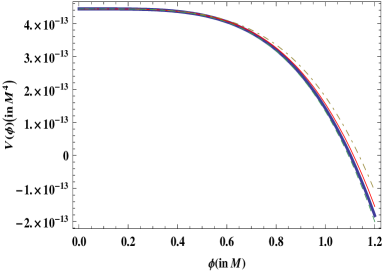
Figure 1: Variation of one loop corrected potential($V(\phi)$) versus inflaton field ($\phi$)

Figure (1) represents the inflaton potential for different values of $C_{4}$, $D_{4}$ and $K_{4}$. From the observational constraints the best fit model is given by the range $-0.70<D_{4}<-0.60$ so that while doing numericals we shall restrict ourselves to this range of $D_{4}$. In what follows our primary intention will be to engage ourselves in modeling brane inflation and to search for its pros and cons with the above potential (1). We shall indeed find that brane inflation with such a potential successfully explains the CMB observations and thus leads to a promising model of inflation.

As already mentioned, the most appealing feature of brane cosmology is that the 4 dimensional Friedmann equations are to some extent different from the standard ones due to the non-trivial embedding in the $S^{1}/Z_{2}$ manifold Maartens . At high energy regime one can neglect the contribution from Weyl term and consequently, the brane Friedmann equations are given by Maartens ; Ellwanger $H^{2}=\frac{8\pi V}{3M^{2}_{PL}}\left[1+\frac{V}{2\lambda}\right]$. The modified Freidmann equations, along with the Klein Gordon equation, lead to new slow roll conditions and new expressions for observable parameters as well Maartens ; Ellwanger . For convenience throughout the analysis we define the following global functions of the inflaton field

$$\begin{array}[]{lllll}L(\phi)=\left[1+\frac{\alpha}{2}S(\phi)\right],~{}~{}~{}~{}T(\phi)=\left[1+\alpha S(\phi)\right],~{}~{}S(\phi)=\left[1+\{D_{4}+K_{4}\ln\left(\frac{\phi}{M}\right)\}\left(\frac{\phi}{M}\right)^{4}\right],\\ U(\phi)=\left[(K_{4}+4D_{4})+4K_{4}\ln\left(\frac{\phi}{M}\right)\right],~{}~{}E(\phi)=\left[(7K_{4}+12D_{4})+12K_{4}\ln\left(\frac{\phi}{M}\right)\right],\\ F(\phi)=\left[(26K_{4}+24D_{4})+24K_{4}\ln\left(\frac{\phi}{M}\right)\right],~{}~{}J(\phi)=\left[(50K_{4}+24D_{4})+24K_{4}\ln\left(\frac{\phi}{M}\right)\right],\\ \tilde{\bar{P}}(\phi)=\sqrt{\left[1+2\alpha S(\phi)L(\phi)\right]}-2\alpha S(\phi)L(\phi)\sinh^{-1}\left(\left[2\alpha S(\phi)L(\phi)\right]\right)^{-1/2}\end{array}$$ (2)

with $\alpha=\Delta^{4}/\lambda$. Incorporating the potential of our consideration from Eq (1) the slow roll parameters turn out to be

$$\epsilon_{V} = \frac{M^{2}_{PL}}{16\pi}\left(\frac{V^{{}^{\prime}}}{V}\right)^{2}\frac{1+\frac{V}{\lambda}}{(1+\frac{V}{2\lambda})^{2}}=\frac{U^{2}(\phi)T(\phi)}{2S^{2}(\phi)L^{2}(\phi)}\left(\frac{\phi}{M}\right)^{6},$$ (3)

$$\eta_{V} = \frac{M^{2}_{PL}}{8\pi}\left(\frac{V^{{}^{\prime\prime}}}{V}\right)\frac{1}{(1+\frac{V}{2\lambda})}=\frac{E(\phi)}{S(\phi)L(\phi)}\left(\frac{\phi}{M}\right)^{2},$$ (4)

$$\xi_{V} = \frac{M^{4}_{PL}}{(8\pi)^{2}}\left(\frac{V^{{}^{\prime}}V^{{}^{\prime\prime\prime}}}{V^{2}}\right)\frac{1}{(1+\frac{V}{2\lambda})^{2}}=\frac{U(\phi)F(\phi)}{S^{2}(\phi)L^{2}(\phi)}\left(\frac{\phi}{M}\right)^{4},$$ (5)

$$\sigma_{V} = \frac{M^{6}_{PL}}{(8\pi)^{3}}\frac{(V^{{}^{\prime}})^{2}V^{{}^{\prime\prime\prime\prime}}}{V^{3}}\frac{1}{(1+\frac{V}{2\lambda})^{3}}=\frac{U^{2}(\phi)J(\phi)}{S^{3}(\phi)L^{3}(\phi)}\left(\frac{\phi}{M}\right)^{6},$$ (6)

,    

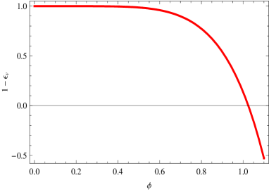
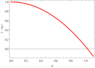
Figure 2: (I) Variation of the 1-$\epsilon_{V}$ vs inflaton field $\phi$ for $C_{4}=-0.68$, (II)Variation of the 1-$|\eta_{V}|$ vs inflaton field $\phi$ for $C_{4}=-0.68$

Figures (2) depict how the first two slow roll parameters vary with the inflaton field for the allowed range of $D_{4}$ and they give us a clear picture of the starting point as well as the end of the cosmic inflation. Nevertheless, Figure (2) further reveals that the $\eta$-problem is smoothened to some extent in brane cosmology. However, we are yet to figure out if there is any underlying dynamics that may lead to the solution of this generic feature of SUGRA.

The number of e-foldings are defined in brane cosmology Maartens for our model as

$$N=\frac{a(t_{f})}{a(t_{i})}\simeq\frac{8\pi}{M^{2}_{PL}}\int^{\phi_{i}}_{\phi_{f}}\left(\frac{V}{V^{{}^{\prime}}}\right)\left(1+\frac{V}{2\lambda}\right)d\phi$$

$$\simeq\frac{M^{2}}{U}\left[\frac{1}{2}\left(1+\frac{\alpha}{2}\right)\left(\frac{1}{\phi^{2}_{f}}-\frac{1}{\phi^{2}_{i}}\right)+\frac{D_{4}}{2M^{4}}(1+\alpha)(\phi^{2}_{i}-\phi^{2}_{f})+\frac{\alpha D^{2}_{4}}{12M^{8}}(\phi^{6}_{i}-\phi^{6}_{f})\right]$$ (7)

which, in the high energy regime, reduces to $N\simeq\frac{\alpha M^{2}}{4|U|}\left[\frac{1}{\phi^{2}_{i}}-\frac{1}{\phi^{2}_{f}}\right]$. Here $\phi_{i}$ and $\phi_{f}$ are the corresponding values of the inflaton field at the start and end of inflation.

Let us now engage ourselves in analyzing quantum fluctuation in our model and its observational imprints via primordial spectra generated from cosmological perturbation Riazuelo . In brane inflation the expressions for amplitude of the scalar perturbation, tensor perturbation and tensor to scalar ratio Maartens ,A.A.Sen ,Wands are given by

$$\Delta^{2}_{s}\simeq\frac{512\pi}{75M^{6}_{PL}}\left[\frac{V^{3}}{(V^{{}^{\prime}})^{2}}\left[1+\frac{V}{2\lambda}\right]^{3}\right]_{k=aH}=\frac{M^{2}\alpha\lambda S^{3}(\phi_{\star})L^{3}(\phi_{\star})}{75\pi^{2}U^{2}(\phi_{\star})(\phi_{\star})^{6}},$$ (8)

$$\Delta^{2}_{t}\simeq\frac{32}{75M^{4}_{PL}}\left[\frac{V\left[1+\frac{V}{2\lambda}\right]}{\left[\sqrt{1+\frac{2V}{\lambda}\left(1+\frac{V}{2\lambda}\right)}-\frac{2V}{\lambda}\left(1+\frac{V}{2\lambda}\right)\sinh^{-1}\left[\frac{1}{\sqrt{\frac{2V}{\lambda}\left(1+\frac{V}{2\lambda}\right)}}\right]\right]}\right]_{k=aH}=\frac{\lambda\alpha}{150\pi^{2}M^{4}}\frac{S(\phi_{\star})L(\phi_{\star})}{\tilde{\bar{P}}(\phi_{\star})},$$ (9)

$$r=16\frac{\Delta^{2}_{t}}{\Delta^{2}_{s}}\simeq\frac{8(\phi_{\star})^{6}U^{2}(\phi_{\star})}{M^{6}S^{2}(\phi_{\star})L^{2}(\phi_{\star})\tilde{\bar{P}}(\phi_{\star})}.$$ (10)

Here and throughout the rest of the article $\phi_{\star}$ represents the value of the inflaton field at the horizon crossing and all the global function defined in eqn(2) is evaluated at the horizon crossing.

   

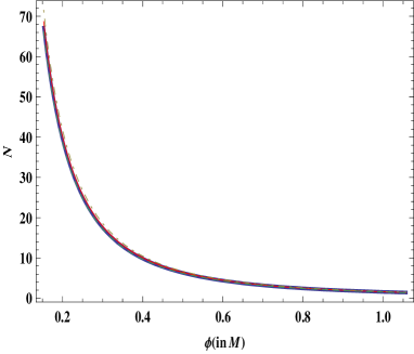
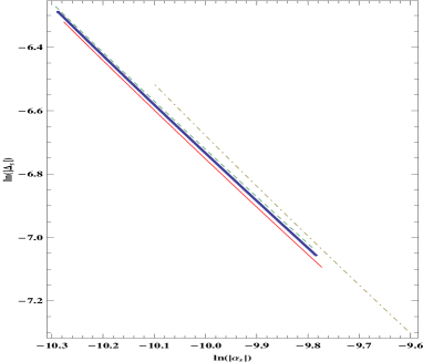
Figure 3:   (I)Variation of the number of e-folding($N$) vs inflation field ($\phi$)(measured in the units of $M$),  (II)Variation of the logarithmic scaled amplitude of the scalar fluctuation ($ln({\Delta}_{s})$) vs logarithmic scaled amplitude of the running of the spectral index ($\ln(|\alpha_{s}|)$)

Figure(3(I)) represents a graphical behavior of number of e-folding versus the inflaton field in the high energy limit for different values of $D_{4}$ and the most satisfactory point in this context is the number of e-folding lies within the observational window $56<N<70$. The end of the inflation leads to the constraint $\alpha=\frac{2}{(|U|)}(|E|)^{\frac{3}{2}}$ which is required for numerical estimations. Here figure(3(II)) represents the logarithmically scaled plots of the physical set of parameter ($\Delta_{s},\alpha_{s}$)for different values of $D_{4}$. The plots themselves present good fit with observations.

Further, the scale dependence of the perturbations, described by the scalar and tensor spectral indices, as follows lythm ,Bassett

$$n_{s}-1=\frac{d(\ln(\Delta^{2}_{s}))}{d(\ln(k))}\simeq(2\eta^{\star}_{V}-6\epsilon^{\star}_{V})=\frac{2E(\phi_{\star})}{S(\phi_{\star})L(\phi_{\star})}\left(\frac{\phi_{\star}}{M}\right)^{2}-\frac{3U(\phi_{\star})T(\phi_{\star})}{S^{2}(\phi_{\star})L^{2}(\phi_{\star})}\left(\frac{\phi_{\star}}{M}\right)^{6},$$

$$~{}~{}~{}~{}n_{t}=\frac{d(\ln(\Delta^{2}_{t}))}{d(\ln(k))}\simeq-3\epsilon^{\star}_{V}=-\frac{3U^{2}(\phi_{\star})T(\phi_{\star})}{2S^{2}(\phi_{\star})L^{2}(\phi_{\star})}\left(\frac{\phi_{\star}}{M}\right)^{6}.$$ (11)

where $d(\ln(k))=Hdt$. Here one can check that santos the validity of the consistency condition $r=24\epsilon_{V}=24\epsilon^{\star}_{V};~{}~{}n_{t}=-3\epsilon_{V}\simeq-3\epsilon^{\star}_{V}=-\frac{r}{8}$.

The expressions for the running of the scalar and tensor spectral index in this specific model with respect to the logarithmic pivot scale at the horizon crossing are given by

$$\alpha_{s}=(16\eta\epsilon-18\epsilon^{2}-2\xi)$$

$$=\frac{8E(\phi_{\star})U^{2}(\phi_{\star})T(\phi_{\star})}{S^{3}(\phi_{\star})L^{3}(\phi_{\star})}\left(\frac{\phi_{\star}}{M}\right)^{8}-\frac{2F(\phi)U(\phi_{\star})}{S^{2}(\phi_{\star})L^{2}(\phi_{\star})}\left(\frac{\phi_{\star}}{M}\right)^{4}-\frac{9U^{4}(\phi_{\star})T^{2}(\phi_{\star})}{2S^{4}(\phi_{\star})L^{4}(\phi_{\star})}\left(\frac{\phi_{\star}}{M}\right)^{12},$$ (12)

$$\alpha_{t}=(6\epsilon\eta-9\epsilon^{2})=\frac{3E(\phi_{\star})U^{2}(\phi_{\star})T(\phi_{\star})}{S^{3}(\phi_{\star})L^{3}(\phi_{\star})}\left(\frac{\phi_{\star}}{M}\right)^{8}-\frac{9U^{4}(\phi_{\star})T^{2}(\phi_{\star})}{4S^{4}(\phi_{\star})L^{4}(\phi_{\star})}\left(\frac{\phi_{\star}}{M}\right)^{12},$$ (13)

One can also calculate the running of the fourth slow roll parameter as $\frac{d\sigma}{d(\ln(k))}=(\epsilon\sigma-2\eta\sigma)$, but its numerical value turns out to be too small to be detected even in near future for which it can treated as consistency condition in brane.

To estimate five dimensional Planck mass from the observational parameters we use the relation $\sqrt{8\pi}M=M_{PL}=\frac{M^{3}_{5}}{\sqrt{\lambda}}\sqrt{\frac{3}{4\pi}}$. and Eq (8) which leads to

$$M_{5}=\sqrt[6]{\frac{800\pi^{4}\Delta^{2}_{s}U^{2}(\phi_{\star})}{\alpha S^{3}(\phi_{\star})L^{3}(\phi_{\star})}}\phi_{\star}.$$ (14)

Finally using the thermodynamic definition of density at the time of reheating $\rho(t_{reh})=\frac{\pi^{2}N^{\star}T^{4}_{brh}}{30}$ in the inflaton decay width $\Gamma_{total}=3H(T^{breh})=3\sqrt{\frac{\rho(t_{reh})}{3M^{2}}\left[1+\frac{\rho(t_{reh})}{2\lambda}\right]}\simeq\frac{\Delta^{6}}{(2\pi)^{3}M^{5}}$ we have estimated the reheating temperature in the braneworld in terms of the five dimensional Planck mass as

$$\begin{array}[]{ll}\displaystyle T^{breh}=\sqrt{\frac{3}{4\pi^{2}}\sqrt{\frac{5}{N^{*}}}\frac{M^{3}_{5}}{M}}\sqrt[4]{\left[\sqrt{1+\frac{64M^{4}\pi^{2}\Gamma^{2}_{total}}{9M^{6}_{5}}}-1\right]}\\ ~{}~{}~{}~{}~{}~{}~{}\displaystyle=\sqrt[4]{\frac{2250\Delta^{2}_{s}U^{2}(\phi_{\star})\phi^{3}_{\star}}{N^{*}M^{2}\alpha S^{3}(\phi_{\star})L^{3}(\phi_{\star})}}\sqrt[4]{\left[\sqrt{1+\frac{2M^{4}\Gamma^{2}_{total}\alpha S^{3}(\phi_{\star})L^{3}(\phi_{\star})}{225\pi^{2}\Delta^{2}_{s}\phi^{6}_{\star}U^{2}(\phi_{\star})}}-1\right]},\end{array}$$ (15)

where $N^{\star}$ is the effective number of particles incorporating the relativistic degrees of freedom.

III parameter estimation

III.1 Direct numerical estimation

$C_{4}$	$\alpha$	$\lambda$	$\phi_{f}$	$\phi_{i}$	$N$	$\phi_{\star}$	$\Delta^{2}_{s}$	$\Delta^{2}_{t}$	$n_{s}$	$n_{t}$	$r$	$\alpha_{s}$	$\alpha_{t}$	$M_{5}$	$T^{breh}$
$\simeq D_{4}$		$\times 10^{-14}M^{4}$	$M$	$M$		$M$	$\times 10^{-9}$	$\times 10^{-14}$		$\times 10^{-5}$	$\times 10^{-5}$	$\times 10^{-3}$	$\times 10^{-6}$	$\times 10^{-3}M$	$\times 10^{-8}M$
				0.147	70	0.158	3.126		0.951	-4.352	2.176	-0.798	-2.125
-0.70	17.389	2.553	1.017	0.158	60	0.173	1.835	6.803	0.941	-7.412	3.706	-1.142	-4.323	11.792	3.119
				0.164	56	0.180	1.440		0.936	-9.447	4.723	-1.345	-5.975
				0.150	70	0.161	2.902		0.951	-4.352	2.176	-0.798	-2.125
-0.65	16.757	2.632	1.036	0.161	60	0.176	1.704	6.317	0.941	-7.412	3.706	-1.142	-4.323	11.865	3.133
				0.167	56	0.184	1.327		0.936	-9.447	4.723	-1.345	-5.975
				0.153	70	0.165	2.679		0.951	-4.352	2.176	-0.798	-2.125
-0.60	16.099	2.758	1.057	0.165	60	0.180	1.573	5.831	0.941	-7.412	3.706	-1.142	-4.323	11.944	3.149
				0.170	56	0.187	1.234		0.936	-9.447	4.723	-1.345	-5.975

Table 1: Different observational parameters related to the cosmological perturbation for our model of inflation including one loop radiative correction

Table 1 represent numerical estimation for different observational parameters related to the cosmological perturbation as estimated from our model. Here a “$\times$” implies “in units of”. It is worthwhile to point out to the salient features of those parameters in the above table as obtained from our model.

• The observable parameters help us have an estimation for the brane tension to be $\lambda\gg(1MeV)^{4}$ provided energy scale of the inflation is in the vicinity of GUT scale and exactly it is of the order of $0.2\times 10^{16}GeV$ which resolves Polonyi problem Coughlan and Gravitino problem Chol .

• The scalar power spectrum corresponding to different best fit values of $D_{4}$ mentioned above is of the order of $5\times 10^{5}$ and it perfectly matches with the observational data wmap07 .

• The scalar spectral index for lower values of $N\rightarrow 55$ are pretty close to observational window $0.948<n_{s}<1$ wmap07 whereas for higher values of $N\rightarrow 70$ this lies well within the window. Thus this small observational window reveals that $N\approx 70$ is more favored in brane cosmology compared to its lower values.

• Though the tensor to scalar ratio as estimated from our model is well within its upper bound fixed by WMAP7 wmap07 ($r<0.45$ at $95\%$ C.L.), thereby facing no contradiction with observations, its value is even small to be detected in WMAP wmap07 or the forthcoming Planck planck . For more discussion see grav .

• For our model running of the scalar spectral index $\alpha_{s}\sim-10^{-3}$ which is quite consistent with WMAP3 wmap3 . Also, the running of the tensor spectral index $\alpha_{t}\sim-6\times 10^{-6}$ may serve as an additional observable parameter to be investigated further.

• Five dimensional Planck mass turns out to be $M_{5}\sim(11.792-11.944)\times 10^{-3}M$ which is the prime input for the estimation of brane reheating temperature as shown in eqn(15). For our model it is estimated as $T^{breh}\sim(3.119-3.149)\times 10^{-8}M$ and clearly depicts the deviation from standard cosmology.

III.2 Data analysis with CAMB

In this context we shall make use of the cosmological code CAMBcamb in order to confront our results directly with observation. To operate CAMB, the values of the initial parameters associated with inflation are taken from the Table1 for $D_{4}=-0.60$. Additionally WMAP7 dataset in $\Lambda$CDM background has been used in CAMB to obtain CMB angular power spectrum at the pivot scale $k_{0}=0.002~{}{\rm Mpc}^{-1}$. Table 3 and table3 shows input from the WMAP7 dataset and the output obtained from CAMB respectively.

$H_{0}$	$\tau_{Reion}$	$\Omega_{b}h^{2}$	$\Omega_{c}h^{2}$	$T_{CMB}$
km/sec/MPc				K
71.0	0.09	0.0226	0.1119	2.725

Table 2: Input parameters in CAMB

$t_{0}$	$z_{Reion}$	$\Omega_{m}$	$\Omega_{\Lambda}$	$\Omega_{k}$	$\eta_{Rec}$	$\eta_{0}$
Gyr					Mpc	Mpc
13.707	10.704	0.2670	0.7329	0.0	285.10	14345.1

Table 3: Output parameters from CAMB

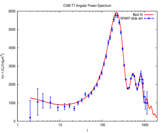
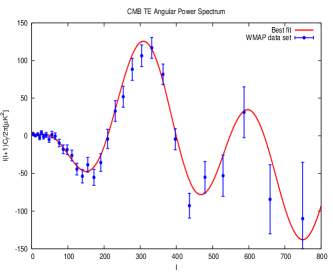
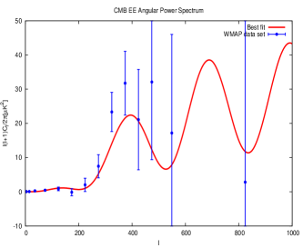
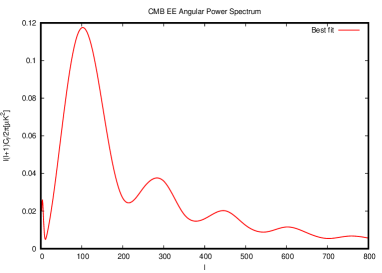
Figure 4: Variation of CMB angular power spectrum (a)$C_{l}^{TT}$, (b)$C_{l}^{TE}$ and (c)$C_{l}^{EE}$ for best fit and WMAP seven years data with the multipoles $l$ for scalar modes

      

      

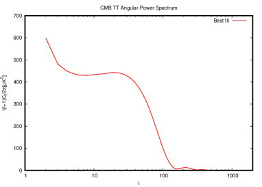
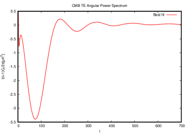
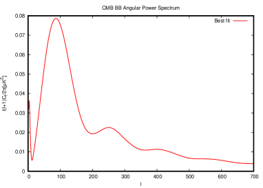
Figure 5: Variation of CMB angular power spectrum (a)$C_{l}^{TT}$, (b)$C_{l}^{TE}$, (c)$C_{l}^{EE}$ and (d)$C_{l}^{BB}$ with the multipoles $l$ for tensor mode

The curvature perturbation is generated due to the fluctuations in the inflaton and at the end of inflation it makes horizon re-entry creating matter density fluctuations, which is the origin of the structure formation in Universe. In Fig.4(a)-Fig4(c) we confront CAMB output of CMB angular power spectrum $C_{l}^{TT}$, $C_{l}^{TE}$ and $C_{l}^{EE}$ for best fit with WMAP seven years data for the scalar mode. From Fig.4(a) we see that the Sachs-Wolfe plateau sachs obtained from our model is almost flat confirming a nearly scale invariant spectrum. For larger value of the multipole $l$, CMB anisotropy spectrum is dominated by the Baryon Acoustic Oscillations (BAO) mukhanovb giving rise to several ups and downs in the spectrum. Also the peak positions are sensitive on the dark energy and other forms of the matter. In Fig.4(a) the first and most prominent peak arises at $l=221$ at a height of $5818{\rm\mu K^{2}}$ followed by two equal height peaks at $l=529$ and $l=822$. This is in good agreement with WMAP7 data for $\Lambda$CDM background apart from the two outliers at $l=21$ and $l=42$. The gravitational waves generated during inflation also remain constant on super Hubble scales having small amplitudes which die off very rapidly due to smaller wavelength than horizon. So the small scale modes have no impact in the CMB anisotropy spectrum only the large scale modes have little contribution and this is obvious from Fig.5(a)-Fig.5(d) where we have plotted the CAMB output of CMB angular power spectrum $C_{l}^{TT}$, $C_{l}^{TE}$, $C_{l}^{EE}$ and $C_{l}^{BB}$ for best fit with WMAP7 data for the tensor mode. Thus, from the entire data analysis with CAMB, it turns out that our model confronts extremely well with WMAP7 dataset and leads to constrain the best fit value of the parameter $D_{4}$ at $-0.60$.

IV Dynamical signature of the model

Let us now engage ourselves in finding out the dynamical signature of the model from the first principle. Precisely, we are interested to obtain a solution of the modified Friedman equation and Klein-Gordon equation in brane cosmology with our proposed model. Under slow-roll approximations the inflaton field as a function of cosmic time can be expressed as

$$\phi(t)=\frac{M^{2}}{\sqrt{2D_{4}}}\sqrt{\left[\tilde{\bar{\Phi}}(f)-\bar{G}t\right]}\sqrt{\left[1-\sqrt{1+\frac{4D_{4}}{M^{4}\left[\tilde{\bar{\Phi}}(f)-\bar{G}t\right]^{2}}}\right]},$$ (16)

where $\bar{G}=\frac{2U\sqrt{2\lambda}}{\sqrt{3}M^{3}},~{}~{}\tilde{\bar{\Phi}}(f)=\frac{1}{\phi^{2}_{f}}\left(\frac{D_{4}\phi^{4}_{fe}}{M^{4}}-1\right)+\bar{G}t_{f}$. It may be noted that in the high energy limit, the above equation(16) reduces to a much tractable form $\phi(t)=\phi_{f}\left[1+\frac{2U\phi^{2}_{f}}{M^{3}}\sqrt{\frac{2\lambda}{3}}(t-t_{f})\right]^{-\frac{1}{2}}$.

    

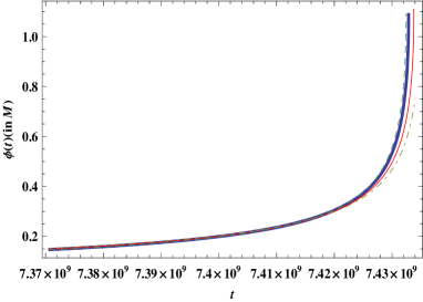
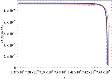
Figure 6: (I) Variation of the inflaton field ($\phi$) with time(t), (II)  Variation of the Hubble parameter ($H(t)$) with time($t$)

Figure (6(I)) shows the evolution of the inflaton field under high energy approximation which shows a smooth increasing behavior of the inflaton field with respect to the inflationary time scale where the span of the scale are within the window $t_{i}<t<t_{f}$. In figure (6(II)) the evolution of the Hubble parameter shows deviations from the de-Sitter as given by the bending of the plots towards the end of inflation which leads to physically more realistic scenario so as to fit with observational data as demonstrated earlier.

Substituting equation(16) in the modified Friedman equation in brane for our model we obtain

$$H(t)=\sqrt{\frac{\lambda}{6}}\frac{\alpha}{M}\left[2+\frac{M^{4}}{2D_{4}}\left[\tilde{\bar{\Phi}}(f)-\bar{G}t\right]^{2}\left(1-\sqrt{1+\frac{4D_{4}}{M^{4}\left[\tilde{\bar{\Phi}}(f)-\bar{G}t\right]^{2}}}\right)\right]$$ (17)

which shows the time evolution as well as the susceptance of Hubble parameter in the context of brane.

Consequently, the solution of the modified Friedman equation, after rearranging terms, gives rise to the scale factor as follows

$$a(t)=a(t_{f})\exp\left[\sqrt{\frac{\lambda}{6}}\frac{\alpha}{M}\left[2(t-t_{f})+\tilde{A}(t-t_{f})+\frac{\tilde{B}}{3}(t^{3}-t^{3}_{f})-\frac{\tilde{C}}{2}(t^{2}-t^{2}_{f})-\tilde{I}(t)\right]\right]$$ (18)

where $\tilde{I}(t)=\int^{t}_{t_{f}}dt\sqrt{\left[(\tilde{A}+\tilde{B}t^{2}-\tilde{C}t+1)^{2}-1\right]},~{}\tilde{A}=\frac{M^{4}\tilde{\bar{\Phi}}(f)}{2D_{4}},\tilde{B}=\frac{\bar{G}^{2}M^{4}}{2D_{4}},~{}\tilde{C}=\frac{\tilde{\bar{\Phi}}(f)\bar{G}M^{4}}{D_{4}}$. Thus the scale factor can be obtained analytically except for the integrand $\tilde{I}(t)$, and it readily shows the deviation from the standard de Sitter model. However, the above form of the scale factor (18) is more or less sufficient to study the dynamical behavior, as represented in Figure(6(II)). As a matter of fact, the leading order contribution from Hubble parameter and the scale factor are indeed closed to de Sitter with the parameters involving brane cosmology.

V Analysis of the energy scale of brane inflation

Let us now estimate the typical scale of inflation in brane cosmology with the potential of our consideration. For this we shall make use of two initial conditions, namely, initial time $t_{i}=0.737\times 10^{10}M^{-1}$ and $a(t_{i})=0.369\times 10^{-1}M^{-1}$. Consequently, for $N=70$ we have $a(t_{f})=0.929\times 10^{11}M^{-1}$. Now taking leading order contribution from Eq (18) the time corresponding to the horizon exit and re-entry can be obtained as

$$t_{\star}=t_{f}+\frac{1}{\bar{G}}\left[\tilde{\bar{\Phi}}(f)-\frac{\left[1\pm\sqrt{1-8D_{4}\left[(\phi_{\star})^{2}+2M^{4}\right]}\right]}{M^{4}}\right],$$ (19)

with $t_{f}=t_{i}+\frac{NM}{\alpha}\sqrt{\frac{6}{\lambda}}$. Using Eq (19), Eq (16) and Eq (4) energy scale of brane inflation can be expressed as

$$\Delta\approx\sqrt[4]{\left[\frac{2E\lambda\phi^{2}_{f}}{|\eta_{V}|M^{2}\left[1+\frac{2U\phi^{2}_{f}}{M^{3}}\sqrt{\frac{2\lambda}{3}}(t-t_{f})\right]}\right]}.$$ (20)

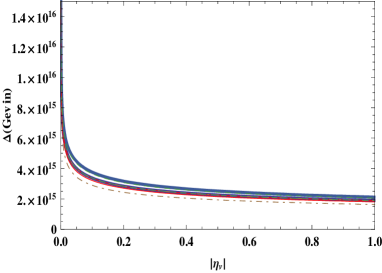
Figure 7: Variation of the energy scale of inflation ($\Delta$) vs $|\eta_{V}|$ including two roots of the horizon crossing time for the best fit model

Figure (7) shows the energy scale of inflation ($\Delta$) versus the magnitude of the second slow roll parameter($|\eta_{v}|$) for different values of the constant $D_{4}$ including two feasible roots of horizon crossing. From the figure it is obvious that for two feasible roots of time corresponding to the horizon crossing an allowed region with finite band-width appears for our proposed model. The above figure further reveals that the typical energy scale of brane inflation with our proposed model is $\Delta\simeq 2\times 10^{15}GeV$ which is supported from cosmological as well as particle physics frameworks.

VI Summary and outlook

In this article we have proposed a model of inflation in brane cosmology. We have demonstrated how we can construct an effective 4D inflationary potential starting from $N=2,D=5$ supergravity in the bulk which leads to an effective $N=1,D=4$ supergravity in the brane. After that we have engaged ourselves in analyzing radiative corrections of the tree level potential and the effective potential calculated from one loop correction has then been employed in estimating the observable parameters, both analytically and numerically, leading to more precise estimation of the quantities and confronting them with WMAP7 dataset using the publicly available code CAMB, which reveals consistency of our model with latest observations. The increase in precision level is worth analyzing considering the advent of more and more sophisticated techniques, both in WMAP wmap07 and in forthcoming Planck planck data.

We have also solved the modified Friedmann equations on the brane leading to an analytical expression for the scale factor during inflation. Finally we have estimated the typical energy scale of brane inflation with the potential of our consideration and found it to be consistent with cosmological as well as particle physics frameworks. This model thus leads to an inflationary scenario in the framework of supergravity inspired brane cosmology.

A detailed survey of thermal history of the universe via reheating, baryogenesis, leptogenesis with the loop corrected potential and gravitino phenomenology remains as an open issue, which may even provide interesting signatures of brane inflation. A detailed analysis on these aspects have been reported as a separate paper reheat .

VII appendix

For systematic development of the formalism, let us demonstrate briefly how one can construct the effective 4D inflationary potential of our consideration starting from $N=2,D=5$ SUGRA in the bulk which leads to an effective $N=1,D=4$ SUGRA in the brane. As mentioned, we consider the bulk to be five dimensional where the fifth dimension is compactified on the orbifold $S^{1}/Z_{2}$ of comoving radius R. The system is described by the following action A.Riotto , kanti

$$S=\frac{1}{2}\int d^{4}x\int^{+\pi R}_{-\pi R}dy\sqrt{g_{5}}\left[M^{3}_{5}\left(R_{(5)}-2\Lambda_{5}\right)+\textit{{L}}_{bulk}+\sum_{i}\delta(y-y_{i})\textit{{L}}_{4i}\right].$$ (21)

Here the sum includes the walls at the orbifold points $y_{i}=(0,\pi R)$ and 5-dimensional coordinates $x^{m}=(x^{\alpha},y)$, where $y$ parameterizes the extra dimension compactified on the closed interval $[-\pi R,+\pi R]$ and $Z_{2}$ symmetry is imposed. For $N=2,D=5$ supergravity in the bulk Eq (21) can be written as

$$S=\frac{1}{2}\int d^{4}x\int^{+\pi R}_{-\pi R}dy\sqrt{g_{5}}\left[M^{3}_{5}\left(R_{(5)}-2\Lambda_{5}\right)+L^{(5)}_{SUGRA}+\sum_{i}\delta(y-y_{i})L_{4i}\right],$$ (22)

which is a generalization of the scenario described in A.Riotto . Written explicitly, the contribution from bulk SUGRA in the action is given by Georg

$$e^{-1}_{(5)}L^{(5)}_{SUGRA}=-\frac{M^{3}_{5}R^{(5)}}{2}+\frac{i}{2}\bar{\Psi}_{i\tilde{m}}\Gamma^{\tilde{m}\tilde{n}\tilde{q}}\nabla_{\tilde{n}}\Psi^{i}_{\tilde{q}}-{S}_{IJ}F^{I}_{\tilde{m}\tilde{n}}F^{I\tilde{m}\tilde{n}}-\frac{1}{2}g_{\alpha\beta}(D_{\tilde{m}}\phi^{\mu})(D^{\tilde{m}}\phi^{\nu})$$

$$+{\rm Fermionic}+{\rm Chern-Simons},$$ (23)

Including the contribution from the radion fields $\chi=-\psi_{5}^{2}$ and $T=\frac{1}{\sqrt{2}}\left(e_{5}^{\dot{5}}-i\sqrt{\frac{2}{3}}A_{5}^{0}\right)$ the effective brane SUGRA counterpart turns out to be

$$\delta(y)L_{4}=-e_{(5)}\Delta(y)\left[(\partial_{\alpha}\phi)^{\dagger}(\partial^{\alpha}\phi)+i\bar{\chi}\bar{\sigma}^{\alpha}D_{\alpha}\chi\right].$$ (24)

Here $\Delta(y)=e^{5}_{\dot{5}}\delta(y)$ is the modified Dirac delta function which satisfies the normalization conditions $\int^{+\pi R}_{-\pi R}dy~{}e^{5}_{\dot{5}}\Delta(y)=1,~{}~{}\int^{+\pi R}_{-\pi R}dy~{}e^{5}_{\dot{5}}={\cal L}$ where ${\cal L}$ is the 5 dimensional volume. The Chern-Simons terms can be gauged away assuming cubic constraints Georg ; Lahanas and $Z_{2}$ symmetry. It is useful to define the five dimensional generalized $K\ddot{a}hler$ function($G$) in this context as Georg ; Lahanas $G=-3\ln\left(\frac{T+T^{\dagger}}{\sqrt{2}}\right)+\delta(y)\frac{\sqrt{2}}{T+T^{\dagger}}K(\phi,\phi^{\dagger})$, which precisely represents interaction of the radion with gauge fields. Including the kinetic term of the five dimensional field $\phi$ the singular terms measured from the modified Dirac delta function can be rearranged into a perfect square thereby leading to the following expression for the action

$$S\supset\frac{1}{2}\int d^{4}x\int^{+\pi R}_{-\pi R}dy\sqrt{g_{5}}e_{(4)}e^{5}_{\dot{5}}\left[g^{\alpha\beta}G_{m}^{n}(\partial_{\alpha}\phi^{m})^{\dagger}(\partial_{\beta}\phi_{n})+\frac{1}{g_{55}}\left(\partial_{5}\phi-\sqrt{H(G)}\Delta(y)\right)^{2}\right],$$ (25)

where $H(G)=\exp\left(\frac{G}{M^{2}}\right)\left[\left(\frac{\partial W}{\partial\phi_{m}}+\frac{\partial G}{\partial\phi_{m}}\frac{W}{M^{2}}\right)^{\dagger}(G_{m}^{n})^{-1}\left(\frac{\partial W}{\partial\phi^{n}}+\frac{\partial G}{\partial\phi^{n}}\frac{W}{M^{2}}\right)-3\frac{|W|^{2}}{M^{2}}\right]$. It is worthwhile to mention that from eqn(25) we can compute energy momentum tensor for $N=2,D=5$ SUGRA can be expressed as

$$T_{\alpha\beta}=G^{n}_{m}(\partial_{\alpha}\phi^{m})^{\dagger}(\partial_{\beta}\phi_{n})-g_{\alpha\beta}\left[g^{\rho\sigma}(\partial_{\rho}\phi^{m})^{\dagger}(\partial_{\sigma}\phi_{n})G^{n}_{m}+g^{55}(\partial_{5}\phi-\sqrt{H(G)}\Delta(y))^{2}\right],$$ (26)

$$T_{55}=\frac{1}{2}(\partial_{5}\phi-\sqrt{H(G)}\Delta(y))^{2}-\frac{1}{2}g_{55}g^{\rho\sigma}G^{n}_{m}(\partial_{\rho}\phi^{m})^{\dagger}(\partial_{\sigma}\phi_{n}).$$ (27)

On the other hand by varying the action written in eqn(25) with respect to the scalar field $\phi$ the equation of motion for $N=2,D=5$ SUGRA can be expressed as

$$\partial_{5}\left[\frac{e^{5}_{\dot{5}}\sqrt{g_{5}}}{g_{55}}(\partial_{5}\phi-\sqrt{H(G)}\Delta(y))\right]+\sum_{n}e^{5}_{\dot{5}}\left\{\partial_{\beta}\left[\sqrt{g_{5}}g^{\alpha\beta}G^{n}_{m}(\partial_{\alpha}\phi^{m})\right]-\frac{\sqrt{g_{5}}}{g_{55}}\Delta(y)\partial_{n}(\sqrt{H(G)})(\partial_{5}\phi-\sqrt{H(G)}\Delta(y))\right\}=0.$$ (28)

Further, imposing $Z_{2}$ symmetry to $\phi$ via $\phi(0)=\phi(\pi R)=0$ and compactifying around a circle $(S^{1})$ $\partial_{5}\phi=\sqrt{H(G)}\left(\Delta(y)-\frac{1}{2\pi R}\right)$ we get,

$$S=\frac{1}{2}\int d^{4}x\int^{+\pi R}_{-\pi R}dy\sqrt{g_{5}}\left[M^{3}_{5}\left(R_{(5)}-2\Lambda_{5}\right)+e_{(4)}e^{5}_{\dot{5}}\left\{g^{\alpha\beta}G_{m}^{n}(\partial_{\alpha}\phi^{m})^{\dagger}(\partial_{\beta}\phi_{n})-g^{55}\frac{H(G)}{4\pi^{2}R^{2}}\right\}\right].$$ (29)

To discuss elaborately the dimensional reduction technique in the regularized fashion here we have to mention the metric structure in $D=5$ in conformal form is given by,

$$ds^{2}_{5}=e^{2A(y)}\left(ds^{2}_{4}+R^{2}\beta^{2}dy^{2}\right),$$ (30)

where the D=4 metric $ds^{2}_{4}=g^{\alpha\beta}dx_{\alpha}dx_{\beta}$ is the well known FLRW metric. The numerical constant $\beta$ has been introduced just for convenience and physically determines the slope of the warp factor $e^{2A(y)}$. Consequently we can express the solution of D=5 Einstein eqns. explicitly in terms of $\beta$ when the warp factor can be expressed as

$$e^{2A(y)}=\frac{b^{2}_{0}}{R^{2}\left(e^{\beta y}+\frac{\Lambda_{5}b^{4}_{0}}{24R^{2}}e^{-\beta y}\right)},$$ (31)

where $b_{0}$ is a constant having dimension of length. Now to trace out all the significant contribution from the fifth dimension using dimensional reduction technique here we use method of separation of variable $\phi^{m}=\phi(x^{\mu},y)=\phi(x^{\mu})\chi(y)$ which leads to,

$$\begin{array}[]{lllll}\displaystyle S=\frac{1}{2}\int d^{4}x\sqrt{g_{4}}\int^{+\pi R}_{-\pi R}dy\left\{\beta M^{3}_{5}Re^{3A(y)}\left[R_{(4)}-\frac{12}{\beta^{2}R^{2}}\left(\frac{dA(y)}{dy}\right)^{2}-\frac{8}{\beta^{2}R^{2}}\left(\frac{d^{2}A(y)}{dy^{2}}\right)-2\Lambda_{5}e^{2A(y)}\right]\right.\\ \left.\displaystyle~{}~{}~{}~{}~{}~{}~{}~{}+\frac{e_{4}}{b_{0}}\Delta(y)(\partial_{\alpha}\phi^{\mu})^{{\dagger}}(\partial^{\alpha}\phi_{\mu})\left(\frac{\partial^{2}K(\phi,\phi^{\dagger})}{\partial\phi^{\dagger}_{\mu}\partial\phi^{\nu}}\right)+C(T,T^{\dagger})\frac{e_{4}}{b_{0}}\frac{\Delta(y)}{4\pi^{2}R^{2}}e^{\frac{K(\phi,\phi^{\dagger})}{M^{2}}}\left[\left(\frac{\partial W}{\partial\phi_{\alpha}}+\left(\frac{\partial K(\phi,\phi^{\dagger})}{\partial\phi_{\alpha}}\right)\frac{W}{M^{2}}\right)^{{\dagger}}\right.\right.\\ \left.\left.~{}~{}~{}~{}~{}~{}~{}~{}~{}~{}~{}~{}~{}~{}~{}~{}~{}~{}~{}~{}~{}~{}~{}~{}~{}~{}~{}~{}~{}~{}~{}~{}~{}~{}~{}~{}~{}~{}~{}~{}~{}~{}~{}~{}~{}~{}~{}~{}~{}~{}~{}~{}~{}~{}~{}~{}~{}~{}~{}~{}~{}~{}~{}\displaystyle\times\left(\frac{\partial^{2}K(\phi,\phi^{\dagger})}{\partial\phi^{\alpha}\partial\phi^{\dagger}_{\beta}}\right)^{-1}\left(\frac{\partial W}{\partial\phi^{\beta}}+\left(\frac{\partial K(\phi,\phi^{\dagger})}{\partial\phi^{\beta}}\right)\frac{W}{M^{2}}\right)-3\frac{|W|^{2}}{M^{2}}\right]\right\},\\ \displaystyle=\frac{1}{2}\int d^{4}x\sqrt{g_{4}}\left\{M^{2}_{PL}\left[R_{(4)}-P\int^{+\pi R}_{-\pi R}dy\frac{4(3e^{2\beta y}+3\lambda^{2}e^{-2\beta y}-2\lambda)}{R^{2}(e^{\beta y}+\lambda e^{-\beta y})^{5}}\right]+\frac{e_{4}}{b_{0}}(\partial_{\alpha}\phi^{\mu})^{{\dagger}}(\partial^{\alpha}\phi_{\mu})\left(\frac{\partial^{2}K(\phi,\phi^{\dagger})}{\partial\phi^{\dagger}_{\mu}\partial\phi^{\nu}}\right)\right.\\ \left.\displaystyle+\frac{e_{4}C(T,T^{\dagger})}{4\pi^{2}R^{2}b_{0}}e^{\frac{K(\phi,\phi^{\dagger})}{M^{2}}}\left[\left(\frac{\partial W}{\partial\phi_{\alpha}}+\left(\frac{\partial K(\phi,\phi^{\dagger})}{\partial\phi_{\alpha}}\right)\frac{W}{M^{2}}\right)^{{\dagger}}\left(\frac{\partial^{2}K(\phi,\phi^{\dagger})}{\partial\phi^{\alpha}\partial\phi^{\dagger}_{\beta}}\right)^{-1}\left(\frac{\partial W}{\partial\phi^{\beta}}+\left(\frac{\partial K(\phi,\phi^{\dagger})}{\partial\phi^{\beta}}\right)\frac{W}{M^{2}}\right)-3\frac{|W|^{2}}{M^{2}}\right]\right\}\\ \displaystyle=\frac{M^{2}_{PL}}{2}\int d^{4}x\sqrt{g_{4}}\left[R_{(4)}-P\int^{+\pi R}_{-\pi R}dy\frac{4(3e^{2\beta y}+3\lambda^{2}e^{-2\beta y}-2\lambda)}{R^{2}(e^{\beta y}+\lambda e^{-\beta y})^{5}}+\left(\frac{\partial^{2}K(\phi,\phi^{\dagger})}{\partial\phi^{\dagger}_{\mu}\partial\phi^{\nu}}\right)(\partial_{\alpha}\phi^{\mu})^{{\dagger}}(\partial^{\alpha}\phi_{\nu})-QV_{F}\right].\end{array}$$ (32)

where $P=\frac{2M^{3}_{5}\beta b^{6}_{0}}{M^{2}_{PL}R^{5}},~{}~{}Q=\frac{C(T,T^{{\dagger}})}{4\pi^{2}R^{2}}$, $M_{PL}=M_{4}=\sqrt{\frac{e_{4}}{b_{0}}}=\sqrt{\frac{6e_{(5)}}{\lambda}}=M^{3/2}_{5}\sqrt{V_{EXTRA}}=\frac{1}{\kappa_{4}}=\sqrt{\frac{6}{\lambda}}\frac{1}{\kappa^{2}_{5}}$, $\lambda=\frac{\Lambda_{5}b^{4}_{0}}{24R^{2}}$ and the compactification volume of the extra dimension $V_{EXTRA}=\frac{3M^{3}_{5}}{4\pi\lambda}$. Here $C(T,T^{\dagger})$ represents an arbitrary function of $T$ and $T^{\dagger}$. So eqn(32) explicitly shows that the theory is reduced to an effective $N=1,D=4$ SUGRA theory. For a general physical situation of $N=1,D=4$ supergravity in the brane where the F-term potential on the brane defined earlier is modified as nills ,Antonio

$$V_{F}=\exp\left(\frac{K(\phi,\phi^{\dagger})}{M^{2}}\right)\left[\left(\frac{\partial W}{\partial\Psi_{\alpha}}+\left(\frac{\partial K}{\partial\Psi_{\alpha}}\right)\frac{W}{M^{2}}\right)^{{\dagger}}\left(\frac{\partial^{2}K}{\partial\Psi^{\alpha}\partial\Psi^{\dagger}_{\beta}}\right)^{-1}\left(\frac{\partial W}{\partial\Psi^{\beta}}+\left(\frac{\partial K}{\partial\Psi^{\beta}}\right)\frac{W}{M^{2}}\right)-3\frac{|W|^{2}}{M^{2}}\right].$$ (33)

Here $\Psi^{\alpha}$ is the chiral superfield and $\phi^{\alpha}$ be the complex scalar field. From now on the inflaton field $\phi$ appears to be 4-dimensional as demonstrated earlier. Consequently for effective $N=1,D=4$ SUGRA eqn(26) and eqn(28) reduces to $T_{\alpha\beta}=\frac{g_{\alpha\beta}e_{4}V_{F}}{2\pi b_{0}R}$ and $\partial_{\beta}\left(\sqrt{g_{4}}\partial^{\beta}\phi\right)+QV^{{}^{\prime}}_{F}(\phi)=0.$ In this context we assume that the K$\ddot{a}$hler potential is dominated by the leading order term (first term) in canonical basis of the series representation i.e. $K=\sum_{\alpha}\phi^{\dagger}_{\alpha}\phi^{\alpha}$. The superpotential in eqn(33) is given by $W=\sum^{\infty}_{n=0}D_{n}W_{n}(\phi^{\alpha})$ with the constraint $D_{0}=1$. Here $W_{n}(\phi^{\alpha})$ is a holomorphic function of $\phi^{\alpha}$ in the complex plane. Consequently in the canonical basis eqn(32) takes the following form

$$S=\frac{M^{2}_{PL}}{2}\int d^{4}x\sqrt{g_{4}}\left[R_{(4)}-P\int^{+\pi R}_{-\pi R}dy\frac{4(3e^{2\beta y}+3\lambda^{2}e^{-2\beta y}-2\lambda)}{R^{2}(e^{\beta y}+\lambda e^{-\beta y})^{5}}+(\partial_{\alpha}\phi^{\mu})^{{\dagger}}(\partial^{\alpha}\phi_{\mu})-QV_{F}\right],$$ (34)

where the F-term potential can be recast as ($V_{D}=0\Leftrightarrow U(1)$ gauge interaction is absent) M.C.Bento

$$V=V_{F}=\exp\left[\frac{1}{M^{2}}\sum_{\alpha}\phi^{\dagger}_{\alpha}\phi^{\alpha}\right]\left[\sum_{\beta}\left|\frac{\partial W}{\partial\phi_{\beta}}\right|^{2}-3\frac{|W|^{2}}{M^{2}}\right].$$ (35)

Now we expand the slowly varying inflaton potential derived from F-term around the value of the inflaton field where the quantum fluctuation is governed by, $\phi\rightarrow\tilde{\phi}+\phi$, ($\tilde{\phi}$ being the value of the inflaton field where structure formation occurs) and by imposing $Z_{2}$ removing all odd order term responsible for gravitational instabilities the required renormalizable inflaton potential turns out to be Adams $V=\Delta^{4}\sum^{2}_{m=0}C_{2m}\left(\frac{\phi}{M}\right)^{2m}$, with another constraint $C_{0}=1$. The mass term decides the steepness of the potential. Absence of this term indicates that process is slow which is compensated by brane tension in the braneworld scenario riotto . For the phenomenological purpose this specific choice is completely viable. But to incorporate thermal history of the universe leading to reheating and baryogenesis among others we need to perform the one loop corrected finite temperature extension Narlikar of our model. Now translating the momentum integral within a specified cut-off ($\Lambda$) the effective potential turns out to be

$$V(\phi)=\Delta^{4}+\frac{g}{4!}\phi^{4}+\frac{g^{2}\phi^{4}}{(16\pi)^{2}}\left[\ln\left(\frac{\phi^{2}}{\Lambda^{2}}\right)-\frac{25}{6}\right]+O(\lambda^{3}),$$ (36)

where the coupling constant $g=\frac{24\Delta^{4}C_{4}}{M^{4}}$ (Here $C_{4}$ is a tree level constant) which ryder is, in general, defined as $g(M)=\frac{d^{4}V(\phi)}{d\phi^{4}}|_{\phi=M}=g+\frac{g^{2}}{(8\pi)^{2}}\left[6\ln(\frac{M^{2}}{\Lambda^{2}})\right]+O(g^{3})$ so that the general expression for the effective potential in terms of all finite physical parameters is given by

$$V(\phi)=\Delta^{4}+\frac{g(M)}{4!}\phi^{4}+\frac{g^{2}(M)\phi^{4}}{(16\pi)^{2}}\left[\ln(\frac{\phi^{2}}{M^{2}})-\frac{25}{6}\right]+O(g(M)^{3}).$$ (37)

which is the Coleman Weinberg potential Coleman ,Landau . After substituting the expression for $g$ in terms of $C_{4}$ the one loop corrected potential can be expressed as

$$V(\phi)=\Delta^{4}\left[1+\left(D_{4}+K_{4}\ln\left(\frac{\phi}{M}\right)\right)\left(\frac{\phi}{M}\right)^{4}\right],$$ (38)

where $K_{4}=\frac{9\Delta^{4}C^{2}_{4}}{2\pi^{2}M^{4}},~{}~{}D_{4}=C_{4}-\frac{25K_{4}}{12}$. This is precisely the potential eqn(1) mentioned in inflationary model building in the present paper.

References

• (1) H. P. Nilles, Phys. Rept. (1984) 110.
• (2) D. H. Lyth and A. Riotto , Phys. Rept. (1999) 314 and references therein.
• (3) M. Kawasaki, M. Yamaguchi, and T. Yanagida, Phys. Rev. Lett.85(2000)3572; M. Yamaguchi and J. Yokoyama, Phys. Rev.D 63(2001)043506; P. Brax and J. Martin, Phys. Rev. D 72(2005)023518.
• (4) P. Binetruy and M. K. Gaillard, Phys. Lett. B 195(1987)382; M. K. Gaillard, H. Murayama and K. A. Olive, Phys. Lett. B 355(1995) 71 77; M. K. Gaillard, D. H. Lyth, and H. Murayama, Phys. Rev. D 58(1998) 123505.
• (5) L. Covi, M. Gomez-Reino, C. Gross, J. Louis, G. A. Palma and C. A. Scrucca JHEP 0808 (2008) 055.
• (6) L. Randall and R. Sundrum, Phys. Rev. Lett. 83, 3370 (1999); L. Randall and R. Sundrum, Phys. Rev. Lett. 83, 4690 (1999).
• (7) R. Maartens and K. Koyama, Living Rev. Relativity 13, (2010) 5.
• (8) H. A. Bridgman, K. A. Malik and D. Wands, Phys. Rev. D65 (2002) 043502.
• (9) R. Maartens, Phys. Rev. D62 (2000) 084023; C. Gordon and R. Maartens, Phys. Rev. D63 (2001) 044022; B. Leong, P. K. S. Dunsby, A. D. Challinor and A. N. Lasenby, Phys. Rev. D65 (2002) 104012; B. Gumjudpai, R. Maartens and C. Gordon, Class. Quant. Grav. 20 (2003) 3592; N. Goheer, P.K.S. Dunsby, A. Coley and M. Bruni, Phys. Rev. D70, 123517 (2004).
• (10) D. Langlois, R. Maartens, M. Sasaki and D. Wands, Phys. Rev. D63 (2001) 084009.
• (11) K. Koyama, Phys. Rev. D66 (2002) 084003; J. D. Barrow and R. Maartens, Phys. Lett. B532 (2002) 153.
• (12) R. Maartens, in Reference Frames and Gravitomagnetism, ed. J. F. Pascual-Sanchez et al. (World Sci.) (2001) 93.
• (13) B. Leong, A. D. Challinor, R. Maartens and A. N. Lasenby, Phys. Rev. D66 (2002) 104014.
• (14) J. Soda and S. Kanno, Phys. Rev. D66 (2002) 083506; T. Shiromizu and K. Koyama, Phys. Rev. D67 (2003) 084022.
• (15) Y. Himemoto and M. Sasaki, Phys. Rev. D63 (2001) 044015; N. Sago, Y. Himemoto and M. Sasaki, Phys. Rev. D65 (2001) 024014; S. Kobayashi, K. Koyama and J. Soda, Phys. Lett. B 501 (2001) 157.
• (16) R. Maartens, D. Wands, B. A. Bassett and I. P. C. Heard, Phys. Rev. D 62 (2000) 041301.
• (17) M. C. Bento, N. M. C. Santos and A. A. Sen, Phys .Rev .D 69, (2004), 023508.
• (18) N. Jones, H. Stoic and, S.-H.Henry Tye, JHEP 0207 (2002) 051; H. P. Nilles, K. A. Olive and M. Peloso, Phys. Lett. B 522 (2001) 304; J. E. Kim, H. P. Nilles and M. Peloso, JCAP 0501 (2005) 005.
• (19) S. Forste, Z. Lalak, S. Lavignac and H. P. Nilles, Phys. Lett. B 481 (2000) 360; H. P. Nilles, A. Papazoglou and G. Tasinato, Nucl. Phys. B 677 (2004) 405.
• (20) S. Forste, Z. Lalak, S. Lavignac and H. P. Nilles, JHEP 0009 (2000) 034.
• (21) J. E. Kim and H. P. Nilles, Phys. Lett. B 553 (2003) 1; J. E. Kim and H, P. Nilles, JCAP 0905, 010 (2009).
• (22) W. D. Goldberger and M. B. Wise, Phys. Rev. Lett. 83, 4922 (1999).
• (23) James M. Cline, C. Grojean and G. Servant, Phys. Rev. Lett. 83 (1999) 4245.
• (24) G. A. Diamandis, B. C. Georgalas, P. Kouroumalou and A. B. Lahanas, Phys. Lett. B602, 112 (2004).
• (25) G. A. Diamandis, B. C. Georgalas, P. Kouroumalou and A. B. Lahanas , Phys. Lett.B660, 247 (2008).
• (26) G. Dvali, Q. Shafi and R. Schaefer, Phys.Rev.Lett. 73 (1994) 1886.
• (27) S. Kachru, R. Kallosh, A. Linde, J. Maldacena, L. McAllister and S. P. Trivedi, JCAP 0310, 013 (2003) ; D. Baumann, A. Dymarsky, I. R. Klebanov, L. McAllister and P. J. Steinhardt, Phys.Rev.Lett. 99 (2007) 141601 ; D. Baumann, A. Dymarsky, I. R. Klebanov, L. McAllister, JCAP 0801 (2008) 024.
• (28) WMAP collaboration, D. N. Spergel et al., Astrophys. J. Suppl. 170, 377 (2007); for uptodate results on WMAP, see http://lambda.gsfc.nasa.gov/product/map/current.
• (29) Planck collaboration, http://www.rssd.esa.int/index.php?project=Planck , some early results are also available, see, for example, P. A. R. Ade et.al., arXiv:1101.2022.
• (30) CAMB, Online link: http://camb.info/.
• (31) S. Coleman and E. Weinberg, Phys. Rev. D 7 (1973) 1888.
• (32) L.D. Landau, Zh. Elsp. Teor. Fiz. 7, (1937) 627; H. Kleinert, Phys. Lett. B 128, 69 (1983).
• (33) A. Das, Lectures of Quantum Field Theory , World Scientific (2008).
• (34) L. H. Ryder, Quantum Field Theory, Cambridge University Press (2008).
• (35) P. Binetruy, C. Deffayet, U. Ellwanger and D. Langlois, Phys. Lett. B 477 (2000) 285; T. Shiromizu, K. Maeda and M. Sasaki, Phys. Rev. D 62 (2000) 024012. E. E. Flanagan, S. H. Tye and I. Wasserman, Phys. Rev. D 62(2000) 044039; M. Gasperini, Elements of String Cosmology , Cambridge University Press (2007).
• (36) R. Maartens, arXiv:astro-ph/0402485.
• (37) D. Langlois, R. Maartens and D. Wands, Phys. Lett. B 489 (2000) 259; K. Koyama and J. Soda, Phys. Rev. D 62 (2000) 123502.
• (38) A. R. Liddle and D. H. Lyth , Cosmological Inflation and Large-Scale Structure, Cambridge University Press (2000).
• (39) M. C. Bento, R. Gonzalez Felipe and N. M. C. Santos, Phys. Rev. D 69 (2004) 123513; M. C. Bento, R. Gonzalez Felipe and N. M. C. Santos, Phys. Rev. D74 (2006) 083503.
• (40) G. D. Coughlan, W. Fischler, E.W. Kolb, S. Raby and G. G. Ross, Phys. Lett. B 131 (1983) 59; J. Ellis, D.V. Nanopoulos and M. Quiros, Phys. Lett. B 174 (1986) 176; B. de Carlos, J.A. Casas, F. Quevedo and E. Roulet, Phys. Lett. B 318 (1993) 447; T. Banks, M. Berkooz, S. H. Shenker, G. Moore and P. J.Steinhardt, Phys. Rev. D 52 (1995) 3548.
• (41) M. Dine and A. E. Nelson, Phys. Rev. D 48, 1277 (1993); U. Chattopadhyay and P. Nath, Phys. Rev. D 53, 1648 (1996); T. Moroi, Phys. Rev. D 53, 6565 (1996, Erratum-ibid. D 56, 4424 (1997).
• (42) D. Baumann et.al., AIP Conf. Proc. 1141 (2009) 10.
• (43) M. Tegmark et. al., Phys. Rev. D 69, 103501 (2004).
• (44) R. K. Sachs and A. M. Wolfe, Astrophys. J. 147, 73 (1967).
• (45) V. F. Mukhanov, Physical Foundation of Cosmology, Cambridge University Press, U.K.(2006).
• (46) S. Choudhury and S. Pal, Nucl. Phys. B 857 (2012) 85 [arXiv:1108.5676].
• (47) A. Riotto and L. Scarabello, JHEP 0205 (2002) 057.
• (48) P. Kanti, I. I. Kogan, K. A. Olive and M. Pospelov , Phys. Lett. B 468 (1999) 31; E. A. Mirabelli and M. E. Peskin, Phys. Rev. D 58 (1998) 065002; C. Csaki, M. Graesser, L. Randall and J. Terning , Phys. Rev. D 62 (2000) 045015.
• (49) M. C. Bento, O. Bertolami and A. A. Sen, Phys. Rev. D 67 (2003) 023504.
• (50) J. A. Adams , G. G. Ross and S. Sarkar , Phys.Lett. B 391 (1997) 271; G. G. Ross and S. Sarkar , Nucl. Phys. B 461 (1996) 597.
• (51) A. Riotto, FERMILAB-PUB - 97/234-A.
• (52) J.V. Narlikar and T. Padmanabhan, Annu. Rev. Astron. Astrophys. 29(1991) 325.