Identity method - a new tool for studying chemical fluctuations

Abstract

Event-by-event fluctuations of the chemical composition of the hadronic system produced in nuclear collisions are believed to be sensitive to properties of the transition between confined and deconfined strongly interacting matter.

In this paper a new technique for the study of chemical fluctuation, the identity method, is introduced and its features are discussed. The method is tested using data on central Pb-Pb collisions at 40$A$ GeV registered by the NA49 experiment at the CERN SPS.

I Introduction

The most interesting features of the phase diagram of strongly interacting matter are the Critical Point (CP) and the $1^{st}$ order phase transition line. Event-by-event fluctuations of the chemical composition of the hadronic system produced in nuclear collisions are believed to be sensitive to both of them. The first relevant measurements were performed by the NA49 experiment at the CERN SPS. A systematic scan in beam energy and system size was recently started by the NA61 collaboration. Furthermore, additional insight is expected from the RHIC beam energy scan program.

There are several measures used to quantify chemical fluctuations, among them: $\sigma_{dyn}$ sigma_dyn ; kpi_fluct_na49 ; dima_cpod2009 used by NA49 and $\nu_{dyn}$ nu_dyn_STAR used by STAR. Both are related as $\sigma_{dyn}^{2}\approx\nu_{dyn}$ and share the same disadvantage, namely, they depend on volume (number of wounded nucleons) and volume fluctuations in thermodynamical (wounded nucleon) models. Another measure $\Phi_{x}$ phi ; Marek was used by NA49 to characterize transverse momentum phipt_syssize ; phipt_energy , electric charge delta_q and azimuthal angle fluctuations phiphi . It is free of the mentioned disadvantage of $\sigma_{dyn}$, $\nu_{dyn}$. However, all these measures of chemical fluctuations are affected by non-perfect particle identification. This is illustrated in Fig. 1 (left panel), where the spectrum of the specific energy loss (dE/dx) of particles measured by the NA49 Time Projection Chambers nim is shown for a selected phase-space bin. The dE/dx signal depends on the particle mass and together with the particle charge measurement is used to identify particles. It is seen that the dE/dx distributions of different particle species partly overlap and thus unique particle identification is not possible.

The identity method adapts the $\Phi_{x}$ measure to take into account a non-unique particle identification, while keeping the advantages of $\Phi_{x}$.

II Identity method

Let us assume that particles are identified according to their measured mass. The measured mass spectra of all particles and of particles of type $h$ in the analyzed event sample are denoted as $\rho$ and $\rho_{h}$, respectively. The spectra are normalized to the corresponding mean multiplicities per event, namely:

$$\int dm\,\rho(m)=\langle N\rangle$$ ,  .

(1)

Furthermore, we define a single particle variable called the particle identity as:

$$w_{h}(m)\buildrel\rm def\over{=}\frac{\rho_{h}(m)}{\rho(m)}~{}.$$ (2)

The fluctuation measure $\Psi_{wh}$ is then introduced in a way similar (the roots over the two components are absent) to the $\Phi$ measure. First, a single particle variable $z$ is defined as:

$$z\buildrel\rm def\over{=}w_{h}-\overline{w_{h}}~{},$$ (3)

where the bar denotes the inclusive mean and thus $\overline{w}=\langle N_{h}\rangle/\langle N\rangle~{}.$ Second, an event variable $Z$, which is the multiparticle analog of $z$, is calculated as:

$$Z\buildrel\rm def\over{=}\sum_{i=1}^{N}(w_{h}(m_{i})-\overline{w_{h}})~{},$$ (4)

where $N$ is the multiplicity and $i$ is the particle index in an event.
Finally, the fluctuation measure $\Psi_{wh}$ is defined as:

$$\Psi_{wh}\buildrel\rm def\over{=}\frac{\langle Z^{2}\rangle}{\langle N\rangle}-\overline{z^{2}}~{}.$$ (5)

For further analysis one denotes two possible values of $\Psi_{wh}$:

• $\Psi_{res}$ which is the value of $\Psi_{wh}$ for the experimental mass resolution case,

• $\Psi_{corr}$ which is the value of $\Psi_{wh}$ for the perfect mass resolution case.

In order to correct for the non-unique particle identification we calculate the variance per particle due to random identification for the experimental mass resolution case:

$$Var_{res}=\frac{1}{\langle N\rangle}\int_{0}^{\infty}dm\,\rho(m)\cdot w_{h}(m)(1-w_{h}(m))~{}.$$ (6)

It is easy to show that for unique particle identification (the perfect mass resolution case, $w_{h}(m)=\delta(m-m_{h})$) the result is $Var_{res}\buildrel\rm def\over{=}Var_{A}=0$, whereas for no mass resolution ( $w_{h}(m)=const.$ ) one obtains $Var_{res}\buildrel\rm def\over{=}Var_{B}=\frac{\langle N_{h}\rangle}{\langle N\rangle}(1-\langle N_{h}\rangle/\langle N\rangle)$. For the experimental data analysis the integral in Eq. 6 is replaced by a sum over all particles.
The following key relation can be proven :

$$\Psi_{corr}=\Psi_{res}(1-Var_{res}/Var_{B})^{-2}~{}.$$ (7)

It shows that the measured fluctuations $\Psi_{res}$ can be corrected for the effect of non-unique particle identification in a model independent way. This is because the correction factor, $(1-Var_{res}/Var_{B})^{-2}$, depends only on the experimental resolution and mean particle multiplicities.

Equation 7 was checked by numerous Monte Carlo simulations with different types of correlations, mass resolution functions and mean particle multiplicities. The results of these simulations are shown in Fig. 1 (right panel).

III The identity method test using NA49 data

In the analysis of experimental data we use the particle energy loss $dE/dx$ as the measure of the mass $m$. For optimal identification the dE/dx spectra from the NA49 TPCs are determined in bins of total and transverse momentum, azimuthal angle as well as for both electric charges separately sigma_dyn ; kpi_fluct_na49 ; dima_cpod2009 . In each bin four Gauss functions (for electrons, pions, kaons and protons) are fitted. An example of such a fit is displayed in Fig. 1 (left panel). The fitted functions are then used as the $\rho_{h}$ and $\rho$ functions of the identity method. The further analysis steps are as follows:

• using mean particle multiplicities the variance $Var_{B}=\langle N_{h}\rangle/\langle N\rangle(1-\langle N_{h}\rangle/\langle N\rangle)$ is obtained,

• for each particle its identity is calculated

  $$w_{hi}(<dE/dx>_{i}|q,p_{tot},p_{T},\phi)=\frac{\rho_{h}(<dE/dx>_{i}|q,p_{tot},p_{T},\phi)}{\rho(<dE/dx>_{i}|q,p_{tot},p_{T},\phi)}~{},$$ (8)

• using the experimental dE/dx resolution functions, $\rho_{h}$ and $\rho$ (M is the total number of particles used in the analysis) the variance

  $$Var_{res}=\frac{1}{M}\sum_{1}^{M}w_{hi}(<dE/dx>_{i}|q,p_{tot},p_{T},\phi)(1-w_{hi}(<dE/dx>_{i}|q,p_{tot},p_{T},\phi))~{},$$ (9)

  is computed,

• using the identity values, $w_{hi}$, $\Psi_{res}$ is calculated and

• the corrected value of $\Psi_{corr}$ is obtained using Eq. 7.

As a first test of the identity method proton fluctuations were studied in Pb+Pb collisions at 40$A$ GeV energy. Positively and negatively charged particles with total momentum up to 40 GeV/c and transverse momentum up to 2 GeV/c were used for the analysis. The total number of analyzed events was 4000. The mean multiplicities are $<N>=165.40$, and $<N_{p}>=42.16$. The obtained value of $\Psi_{res}\cdot 1000=-17.4\pm 3.5$. The corresponding correction factor for non-unique particle identification was calculated to be $\approx 1.2$.
The value corrected for the finite resolution is $\Psi_{corr}\cdot 1000=-22.3\pm 4.4$. The analysis of Pb+Pb collisions at all NA49 energies is in progress.

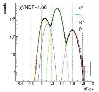
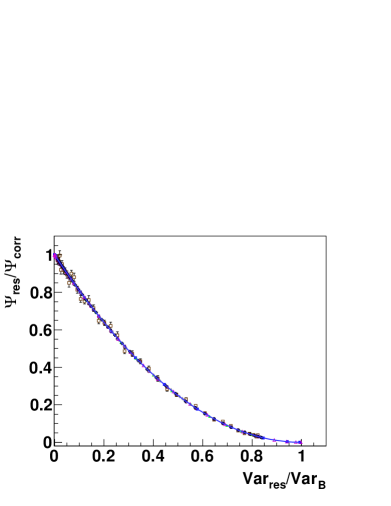
Figure 1: Left panel: Distribution of specific energy loss measured in the NA49 TPCs for positively charged particles is a bin $p_{tot}\epsilon(4.4-5.3)$ GeV/c, $p_{T}\epsilon(0.0-0.2)$ GeV/c and $\phi\epsilon(0.75\pi-\pi)$. The fitted Gauss functions are shown by solid curves. Right panel: The ratio $\Psi_{res}/\Psi_{corr}$ versus $Var_{res}/Var_{B}$ calculated within several Monte Carlo simulations with different parameters of experimental resolution, particle multiplicities and fluctuations. The results agree with the analytical dependence given by Eq. 7.

FIGURE CAPTIONS

1. Left panel: Distribution of specific energy loss measured in the NA49 TPCs for positively charged particles is a bin $p_{tot}\epsilon(4.4-5.3)$ GeV/c, $p_{T}\epsilon(0.0-0.2)$ GeV/c and $\phi\epsilon(0.75\pi-\pi)$. The fitted Gauss functions are shown by solid curves. Right panel: The ratio $\Psi_{res}/\Psi_{corr}$ versus $Var_{res}/Var_{B}$ calculated within several Monte Carlo simulations with different parameters of experimental resolution, particle multiplicities and fluctuations. The results agree with the analytical dependence given by Eq. 7.

References

- (1) S. V. Afanasev et al. (NA49 Collaboration), Phys. Rev. Lett. 86, 1965 (2001).
- (2) C. Alt et al. (NA49 Collaboration), Phys. Rev. C 79, 044910 (2009).
- (3) D. Kresan (for the CBM and NA49 Collaborations), PoS CPOD2009, 031 (2009) [arXiv:0908.2875].
- (4) B. I. Abelev et al. (STAR Collaboration), Phys. Rev. Lett. 103, 092301 (2009).
- (5) M. Gazdzicki, S. Mrowczynski, Z. Phys. C54, 127-132 (1992).
- (6) M. Gaździcki, Eur. Phys. J. C8, 131-133 (1999).
- (7) T. Anticic et al. (NA49 Collaboration), Phys. Rev. C 70, 034902 (2004).
- (8) T. Anticic et al. (NA49 Collaboration), Phys. Rev. C 79, 044904 (2009).
- (9) C. Alt et al. (NA49 Collaboration), Phys. Rev. C 70, 064903 (2004).
- (10) T. Cetner, K. Grebieszkow, S. Mrówczyński arXiv:1011.1631v1
- (11) S. Afanasev et al. (NA49 Collaboration), Nucl. Instrum. Meth. A430, 210-244 (1999).