Bayesian Inference in the Scaling Analysis of Critical Phenomena

Abstract

To determine the universality class of critical phenomena, we propose a method of statistical inference in the scaling analysis of critical phenomena. The method is based on Bayesian statistics, most specifically, the Gaussian process regression. It assumes only the smoothness of a scaling function, and it does not need a form. We demonstrate this method for the finite-size scaling analysis of the Ising models on square and triangular lattices. Near the critical point, the method is comparable in accuracy to the least-square method. In addition, it works well for data to which we cannot apply the least-square method with a polynomial of low degree. By comparing the data on triangular lattices with the scaling function inferred from the data on square lattices, we confirm the universality of the finite-size scaling function of the two-dimensional Ising model.

I Introduction

A wide variety of systems exhibit critical phenomena. Near a critical point, some quantities obey scaling laws. As an example, consider

$$A(t,h)=t^{x}\Psi(ht^{-y}),$$ (1)

where $t$ and $h$ are variables describing a system, and the critical point is located at $t=h=0$. The scaling law is derived by the renormalization group argumentGoldenfeld (1992); *cardy96:_scalin_and_renor_in_statis_physic. The scaling exponents $x$ and $y$ are called critical exponents. The universality of critical phenomena means that different systems share the same set of critical exponents. Thus, this set defines a universality class of critical phenomena. In addition, the scaling function $\Psi$ also exhibits universality. For example, Mangazeev et al. numerically obtained scaling functions of the Ising models on square and triangular latticesMangazeev et al. (2010). Since Ising models on both lattices belong to the same universality class, the two scaling functions with nonuniversal metric factors are perfectly equal.

An important issue to study critical phenomena is to determine the universality class. The object of scaling analysis is to determine the universality class from data. We assume the scaling law of Eq. (1) for data. If we plot data with rescaled coordinates as $(X_{i},Y_{i})\equiv(h_{i}t_{i}^{-y},t_{i}^{-x}A(t_{i},h_{i}))$, all points must collapse on a scaling function as $Y_{i}=\Psi(X_{i})$. To determine critical exponents, we need a mathematical method to estimate how well all rescaled points collapse on a function for a given set. In other words, we need to estimate the goodness of data collapse. Unfortunately, we do not know the form of $\Psi$ a priori . The conventional method for the scaling analysis is a least-square method while assuming a polynomial. However, it may be difficult to choose the degree of the polynomial for data, because there are overfitting problems associated with increasing the degree. To use a polynomial of low degree, we usually limit the data to a narrow region near a critical point. However, it may require high accuracy. In addition, it may be difficult to obtain a universal scaling function in a wide critical region. Thus, the scaling analysis by the least-square method must be carefully done as shown in the reference Slevin and Ohtsuki (1999).

In this paper, we propose a method of statistical inference in the scaling analysis of critical phenomena. The method is based on Bayesian statistics. Bayesian statistics has been widely used for data analysis Bishop (2006). However, to the best of our knowledge, it has not been applied to the scaling analysis of critical phenomena. In particular, since our method assumes only the smoothness of a scaling function, it can be applied to data for which the least-square method cannot be used.

In Sec. II, we first introduce a Bayesian framework in the scaling analysis of critical phenomena. Next, we propose a Bayesian inference using a Gaussian process (GP) in this framework. In Sec. III, we demonstrate this method for critical phenomena of the Ising models on square and triangular lattices. Finally, we give the conclusions in Sec. IV.

II Bayesian framework and Bayesian inference in scaling analysis

By using two functions $X$ and $Y$ that calculate rescaled coordinates, the scaling law of an observable $A$ can be rewritten as

$$Y(A(\vec{v}),\vec{v},\vec{\theta_{p}})=\Psi(X(\vec{v},\vec{\theta_{p}})),$$ (2)

where $\vec{v}$ denotes the variables describing a system and $\vec{\theta_{p}}$ denotes the additional parameters as critical exponents. Our purpose is to infer $\vec{\theta_{p}}$ so that data $A(\vec{v_{i}}),(1\leq i\leq N)$ obey the scaling law of Eq. (2). In the following, for convenience, we abbreviate $X(\vec{v_{i}},\vec{\theta_{p}})$ and $Y(A(\vec{v_{i}}),\vec{v_{i}},\vec{\theta_{p}})$ to $X_{i}$ and $Y_{i}$, respectively.

When the statistical error of $Y_{i}$ is $E_{i}$, the distribution function of $\{Y_{i}\}$, $P(\vec{Y}|\Psi,\vec{\theta_{p}})$, is a multivariate Gaussian distribution with mean vector $\vec{\Psi}$ and covariance matrix $\mathcal{E}$:

$$P(\vec{Y}|\Psi,\vec{\theta_{p}})\equiv\mathcal{N}(\vec{Y}|\vec{\Psi},\mathcal{E}),$$ (3)

where $(\vec{Y})_{i}\equiv Y_{i}$, $(\vec{\Psi})_{i}\equiv\Psi(X_{i})$, $(\mathcal{E})_{ij}\equiv E_{i}^{2}\delta_{ij}$, and

$$\mathcal{N}(\vec{y}|\vec{\mu},\Sigma)\equiv\frac{1}{\sqrt{|2\pi\Sigma|}}\exp\left(-\frac{1}{2}(\vec{y}-\vec{\mu})^{t}\Sigma^{-1}(\vec{y}-\vec{\mu})\right).$$

Next, we introduce a statistical model for a scaling function as $P(\Psi|\vec{\theta_{h}})$. Here, $\vec{\theta_{h}}$ denotes the control parameters and is referred to as hyper parameters. Then, the conditional probability of $\vec{Y}$ for $\vec{\theta_{p}}$ and $\vec{\theta_{h}}$ is formally defined as

$$P(\vec{Y}|\vec{\theta_{p}},\vec{\theta_{h}})\equiv\int P(\vec{Y}|\Psi,\vec{\theta_{p}})P(\Psi|\vec{\theta_{h}})d\Psi.$$ (4)

According to Bayes’ theorem, a conditional probability of $\vec{\theta_{p}}$ and $\vec{\theta_{h}}$ for $\vec{Y}$ can be written as

$$P(\vec{\theta_{p}},\vec{\theta_{h}}|\vec{Y})={P(\vec{Y}|\vec{\theta_{p}},\vec{\theta_{h}})P(\vec{\theta_{p}},\vec{\theta_{h}})}/{P(\vec{Y})},$$ (5)

where $P(\vec{\theta_{p}},\vec{\theta_{h}})$ and $P(\vec{Y})$ denote the prior distributions of $\vec{\theta_{p}}$ and $\vec{\theta_{h}}$ and that of $\vec{Y}$, respectively. In Bayesian statistics, $P(\vec{\theta_{p}},\vec{\theta_{h}}|\vec{Y})$ is called a posterior distribution of $\vec{\theta_{p}}$ and $\vec{\theta_{h}}$. Using Eq. (5), a posterior probability of $\vec{\theta_{p}}$ and $\vec{\theta_{h}}$ for $\vec{Y}$ can be estimated. This is a Bayesian framework for the scaling analysis of critical phenomena.

In Bayesian statistics, the conventional method of inferring parameters is the maximum a posteriori (MAP) estimate. In this paper, for simplicity, we assume that all prior distributions are uniform. Then,

$$P(\vec{\theta_{p}},\vec{\theta_{h}}|\vec{Y})\propto P(\vec{Y}|\vec{\theta_{p}},\vec{\theta_{h}}).$$ (6)

Therefore, the MAP estimate is equal to a maximum likelihood(ML) estimate with a likelihood function of $\vec{\theta_{p}}$ and $\vec{\theta_{h}}$, defined as

$$\mathcal{L}(\vec{\theta_{p}},\vec{\theta_{h}})=P(\vec{Y}|\vec{\theta_{p}},\vec{\theta_{h}}).$$ (7)

In addition, the confidence intervals of the parameters can be estimated through Eq. (6).

In this framework, the statistical model of a scaling function plays an important role. We start from a polynomial scaling function as $\Psi(X)\equiv\sum_{k}c_{k}X^{k}$. If a coefficient $c_{k}$ is distributed by a probability density $P(c_{k}|\vec{\theta_{h}})$, then $P(\Psi|\vec{\theta_{h}})d\Psi\equiv\prod_{k}P(c_{k}|\vec{\theta_{h}})dc_{k}$. We first consider the strong constraint for $c_{k}$ as $P(c_{k}|\vec{\theta_{h}})\equiv\delta(c_{k}-m_{k})$, where $m_{k}$ is a hyper parameter. Then, $P(\vec{Y}|\vec{\theta_{p}},\vec{\theta_{h}})$ is a multivariate Gaussian distribution with mean vector $\vec{\mu}$ and covariance matrix $\Sigma$:

$$(\vec{\mu})_{i}\equiv\sum_{k}m_{k}{X_{i}}^{k},\quad\Sigma\equiv\mathcal{E}.$$ (8)

Thus, the ML estimate in Eq. (7) is equal to the least-square method. We soften this constraint as $P(c_{k}|\vec{\theta_{h}})\equiv\mathcal{N}(c_{k}|m_{k},\sigma_{k}^{2})$, where $m_{k}$ and $\sigma_{k}$ are hyper parameters. Then, $P(\vec{Y}|\vec{\theta_{p}},\vec{\theta_{h}})$ is again a multivariate Gaussian distribution, and the covariance matrix changes as follows:

$$\Sigma\equiv\mathcal{E}+\Sigma^{\prime},\quad(\Sigma^{\prime})_{ij}\equiv\sum_{k}(X_{i}X_{j})^{k}\sigma_{k}^{2}.$$ (9)

This includes the case of a strong constraint such as $\sigma_{k}^{2}=0$.

To calculate a MAP estimate, a log-likelihood function is used. If a posterior distribution is described by a multivariate Gaussian function as $P(\vec{\theta_{p}},\vec{\theta_{h}}|\vec{Y})\propto\mathcal{N}(\vec{Y}|\vec{\mu},\Sigma)$, the log-likelihood function can be written as

$$\log\mathcal{L}(\vec{\theta_{p}},\vec{\theta_{h}})\equiv-\frac{1}{2}\log\left|2\pi\Sigma\right|-\frac{1}{2}(\vec{Y}-\vec{\mu})^{t}\Sigma^{-1}(\vec{Y}-\vec{\mu}).$$ (10)

Although the likelihood function is nonlinear in parameters $\vec{\theta_{p}}$ and $\vec{\theta_{h}}$, a multidimensional maximization method may be applied to calculate a MAP estimate. Under a strong constraint such as $\sigma_{k}^{2}=0$, the Levenberg-Marquardt algorithm is efficient. Under a weak constraint such as $\sigma_{k}^{2}>0$, we may use an efficient maximization algorithm such as the Fletcher-Reeves conjugate gradient algorithm. In such efficient algorithms, we sometimes need the derivative of Eq. (10) for a parameter $\theta$. Then, we can use the following formula:

$$\frac{\partial\log\mathcal{L}(\vec{\theta_{p}},\vec{\theta_{h}})}{\partial\theta} = -\frac{1}{2}\mathbf{Tr}\left(\Sigma^{-1}\frac{\partial\Sigma}{\partial\theta}\right)$$ (11)

$$- (\vec{Y}-\vec{\mu})^{t}\Sigma^{-1}\frac{\partial(\vec{Y}-\vec{\mu})}{\partial\theta}$$

$$+ \frac{1}{2}(\vec{Y}-\vec{\mu})^{t}\Sigma^{-1}\frac{\partial\Sigma}{\partial\theta}\Sigma^{-1}(\vec{Y}-\vec{\mu}).$$

However, to compute the inverse of a covariance matrix, the computational cost of an iteration is $O(N^{3})$. On the other hand, $O(N^{2})$ for the least-square method. Fortunately, using a high-performance numerical library for linear algebra, we can easily make a code and we can efficiently calculate for some hundred data points. Another method is based on Monte Carlo (MC) samplings. In particular, MC samplings may be useful for the estimate of the confidence intervals of parameters.

We demonstrate the MAP estimate based on Eq. (10) and Eq. (9). Fig. 1 shows the data points rescaled by a MAP estimate. Here, we assume that a scaling function is linear. To show the flexibility of Bayesian inference, we fix $m_{0}=m_{1}=0$. Thus, $\sigma_{0}$ and $\sigma_{1}$ are the only free parameters. We artificially generate mock data so that they obey a scaling law:

$$A(T,L)=L^{-\beta/\nu}\Psi((T-T_{c})L^{1/\nu}),$$ (12)

where $T$ and $L$ denote the temperature and linear dimension of a system, respectively. This is a well-known scaling law for finite-size systems. In Fig. 1, we set $T_{c}=\beta/\nu=1,1/\nu=2$ and $\Psi(X)=2+X$. Then,

$$A_{i}=\frac{2}{L_{i}}+(T_{i}-1)L_{i}+r_{i}/50,$$ (13)

where $r_{i}$ is a Gaussian noise. These mock data are shown in the inset of the left panel of Fig. 1. The right panel of Fig. 1 shows the maximization of a likelihood, when we start from $T_{c}=1/\nu=\beta/\nu=0$ and $\sigma_{0}=\sigma_{1}=2$. The results for $T_{c},\beta/\nu$, and $1/\nu$ are $1.00745$, $0.999008$, and $2.00638$, respectively. They are close to the correct values.

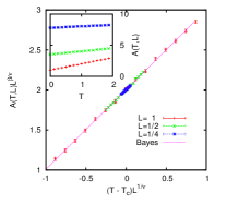
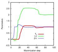
Figure 1: (Color on-line) Left panel: The data points rescaled by a MAP estimate. We assume that a scaling function is linear. The results of the MAP estimate for $T_{c}$, $\beta/\nu$, and $1/\nu$ are $1.00745$, $0.999008$, and $2.00638$, respectively. The dotted (pink) line is the scaling function inferred from the MAP estimate. Inset of left panel: Mock data set. Right panel: Maximization of a likelihood.

Unfortunately, we usually do not know the form of a scaling function a priori . The Bayesian inference based on Eq. (10) and Eq. (9) may not be effective in some cases. Thus, we consider an extension of Eq. (9). From Eq. (10), we may regard data points as obeying a GP. Since the covariance matrix represents statistical correlations in data, we may design it for a wide class of scaling functions. Thus, we introduce a generalized covariance matrix $\Sigma$ as

$$\Sigma=\mathcal{E}+\Sigma^{\prime},(\Sigma^{\prime})_{ij}\equiv K(X_{i},X_{j}),$$ (14)

where $K(X_{i},X_{j})$ is called a kernel function. Note that $\Sigma^{\prime}$ must be a positive definite. The Bayesian inference based on Eq. (10) and Eq. (14) is called a GP regression. Eq. (9) is a special case of Eq. (14). As shown in Fig. 1, even if $\vec{\mu}=0$, the GP regression is successful. For simplicity, we consider only a zero mean vector ($\vec{\mu}=0$) in this paper.

In the GP regression, we can also infer the scaling function. In fact, we assume that all data points obey a GP. In other words, the joint probability distribution of obtained data points and a new additional point $(X,Y)$ is also a multivariate Gaussian distribution. Therefore, a conditional probability of $Y$ for obtained data can be written by a Gaussian distribution with mean $\mu(X)$ and variance $\sigma^{2}(X)$:

$$\mu(X)\equiv\vec{k}^{t}\Sigma^{-1}\vec{Y},\quad\sigma^{2}(X)\equiv K(X,X)-\vec{k}^{t}\Sigma^{-1}\vec{k},$$ (15)

where $(\vec{k})_{i}\equiv K(X_{i},X)$. We regard $\mu(X)$ in Eq. (15) as a scaling function. For example, the dotted (pink) line in Fig. 1 is $\mu(X)$ in Eq. (15) for mock data with a MAP estimate.

In general, a scaling function is smooth. Since $\mu(X)$ in Eq. (15) is the weighted sum of kernel functions, the kernel function should smoothly decrease for increasing distance between two arguments. In this paper, we propose the use of a Gaussian kernel function (GKF) for the scaling analysis of critical phenomena. GKF is defined as

$$K_{G}(X_{i},X_{j})\equiv\theta_{0}^{2}\exp\left(-\frac{(X_{i}-X_{j})^{2}}{2\theta_{1}^{2}}\right),$$ (16)

where $\theta_{0}$ and $\theta_{1}$ are hyper parameters. Since GKF is smooth and local, the GP regression with GKF may be effective for a wide class of scaling functions.

III Bayesian finite-size scaling analysis of the two-dimensional Ising model

We demonstrate the GP regression with GKF for the finite-size scaling (FSS) analysis of the two-dimensional Ising model. FSS is widely used in numerical studies of critical phenomena for finite-size systems. It is based on the FSS law derived by the renormalization group argument. The Hamiltonian of the Ising model can be written as

$$\mathcal{H}(\{s_{i}\})\equiv-J\sum_{\langle ij\rangle}s_{i}s_{j},$$ (17)

where $s_{i}$ is the spin variable ($\pm 1$) of site $i$ and $\langle ij\rangle$ denotes the nearest neighbor pairs and $J$ denotes a positive coupling constant. The partition function can be written as

$$Z\equiv\sum_{\{s_{i}\}}\exp[-H(\{s_{i}\})/k_{B}T],$$ (18)

where $k_{B}$ is the Boltzmann constant. For simplicity, we set $J/k_{B}=1$ in the following. The two-dimensional Ising model has a continuous phase transition at a finite temperature. Since there are exact results for the Ising models on square and triangular latticesOnsager (1944); *1952PhRv...85..808Y, we can check the results of FSS.

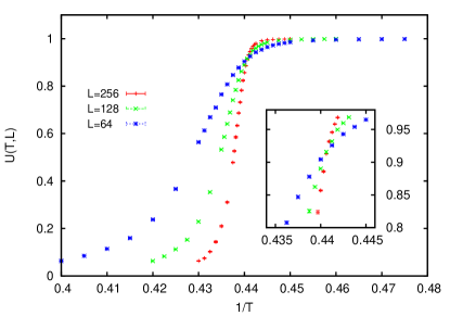
Figure 2: (Color on-line) The Binder ratios of the Ising model on three square lattices. The total number of data items is 86. Inset: Binder ratio near a critical point. The value of the Binder ratio is limited to the region $[0.8,0.97]$. The number of data items in the inset is $24$.

To obtain the Binder ratiosBinder (1981) and magnetic susceptibility on square and triangular lattices, MC simulations have been done.　For the square lattice, $L=L_{r}=64$, $128$, and $256$, where $L_{r}$ and $L$ denote the number of rows and columns of the lattice, respectively. For the triangular lattice, $L=(65L_{r}/75)=65$, $130$, and $260$ so that the aspect ratio of a triangular lattice is approximately $1$. We set periodic boundary conditions for both lattices. The number of MC sweeps by the cluster algorithmSwendsen and Wang (1987) is $80000$ for each simulation. The Binder ratio is based on the ratio of the fourth and second moments of an order parameter. The order parameter of the Ising model is a magnetization defined as $M\equiv\sum_{i}s_{i}$. Then, the Binder ratio can be written as

$$U\equiv\frac{1}{2}\left(3-\frac{\langle M^{4}\rangle}{\langle M^{2}\rangle^{2}}\right),$$ (19)

where $\langle\cdot\rangle$ denotes the canonical ensemble average. In the thermodynamic limit, the Binder ratio takes values 1 and 0 in the order and disorder phases, respectively. Since the Binder ratio is dimensionless, the FSS form is

$$U(T,L)=\Psi_{B}((1/T-1/T_{c})L^{1/\nu}),$$ (20)

where $T_{c}$ is a critical temperature and $\nu$ is a critical exponent that characterizes the divergence of a magnetic correlation length. From Eq. (20), the value of the Binder ratio at the critical temperature is universal. Magnetic susceptibility can be written as

$$\chi\equiv\frac{1}{TV}\left(\langle M^{2}\rangle-\langle M\rangle^{2}\right),$$ (21)

where $V$ is the number of spins. The scaling form of magnetic susceptibility is

$$\chi(T,L)=L^{\gamma/\nu}\Psi_{\chi}((1/T-1/T_{c})L^{1/\nu}),$$ (22)

where $\gamma$ and $\nu$ are critical exponents.

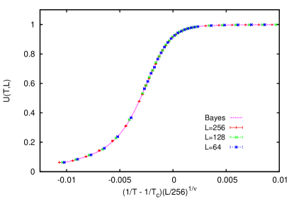
Figure 3: (Color on-line) Result of a Bayesian FSS of the Binder ratio of the Ising model on square lattices. We apply the GP regression with Eq. (23) to the data shown in Fig. 2. The results of the MC estimate are $1/T_{c}=0.440683(7)$ and $1/\nu=0.996(2)$. The dotted (pink) curve is the scaling function inferred from a MAP estimate.

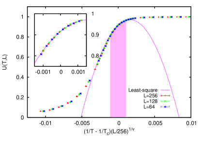
Figure 4: (Color on-line) Result of a FSS of the Binder ratio of the Ising model on square lattices by the least-square method. In the least-square method, we use only the data in the inset of Fig. 2 and assume that the scaling function is a quadratic function. The best estimate of the least-square method is $1/T_{c}=0.44069(2)$ and $1/\nu=1.00(2)$. All data points are rescaled by these values. The data points used in the least-square method are shown in the filled gray (pink) region. The dotted (pink) curve is the scaling function inferred from the best estimate of the least-square method. Inset: Rescaled data points used in the least-square method.

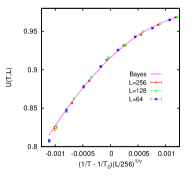
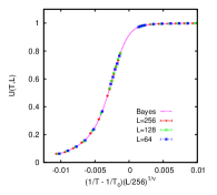
Figure 5: (Color on-line) Left panel: Result of a Bayesian FSS for the data in the inset of Fig. 2. The results of the MC estimate are $1/T_{c}=0.44070(2)$ and $1/\nu=1.00(1)$. Right panel: Result of a Bayesian FSS for data not included in the inset of Fig. 2. The results of the MC estimate are $1/T_{c}=0.440675(9)$ and $1/\nu=0.997(2)$. The dotted (pink) curves in left and right panels are the scaling functions inferred from the MAP estimates.

We first apply the GP regression to the Binder ratios of square lattices shown in Fig. 2. The kernel function based on GKF can be written as

$$K(X_{i},X_{j})\equiv K_{G}(X_{i},X_{J})+\theta_{2}^{2}\delta_{ij},$$ (23)

where a hyper parameter $\theta_{2}$ denotes the data fidelity. We note that the maximization of a likelihood is much improved by $\theta_{2}$. Although $\theta_{2}$ finally goes to zero, it helps to escape from a local maximum of a likelihood. Fig. 3 shows the result of the GP regression for Binder ratios. The results of the MC estimate are $1/T_{c}=0.440683(7)$ and $1/\nu=0.996(2)$. This is consistent with the exact results $1/T_{c}=\ln(1+\sqrt{2})/2=0.4406867925\cdots$ and $1/\nu=1$. The dotted (pink) curve in Fig. 3 is the scaling function inferred from a MAP estimate by using Eq. (15). All points collapse on this curve. The value of the Binder ratio at the critical temperature is $0.9158(4)$. This is consistent with the exact value $0.916038\cdots$Salas and Sokal (2000). It is difficult to represent this curve as a polynomial of low degree. Thus, we limit the value of a Binder ratio to the region $[0.8,0.97]$ (see the inset of Fig. 2). We apply the least-square method with a quadratic function to the limited data. The result is shown in Fig. 4. The inset of Fig. 4 shows the data points rescaled by the best estimate of the least-square method. All points in the inset collapse on a quadratic function (see the dotted (pink) curve in Fig. 4). The reduced chi-square is $2.96$. The results of the least-square method are $1/T_{c}=0.44069(2)$ and $1/\nu=1.00(2)$. This is consistent with the exact result. However, it may be difficult to extend the region of data for the least-square method. The main panel of Fig. 4 shows all data points rescaled by the best estimate of the least-square method. While all points again collapse on a smooth curve, the curve is not equal to the quadratic function outside the limited region (see the filled gray (pink) region in Fig. 4). The left panel in Fig. 5 shows the result of the GP regression to the same data for the least-square method. The results of the MC estimate are $1/T_{c}=0.44070(2)$ and $1/\nu=1.00(1)$. This is consistent with the exact results and similar to that of the least-square method. The GP regression with GKF assumes only the smoothness of a scaling function. Thus, it may be effective even for the data not near a critical point. In fact, even if we use only data not included in the inset of Fig. 2, we can do FSS by the GP regression. The result is shown in the right panel in Fig. 5. The results of the MC estimate are $1/T_{c}=0.440675(9)$ and $1/\nu=0.997(2)$. Although we do not use the important data near a critical point, the result of the GP regression is close to the exact result.

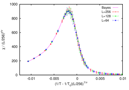
Figure 6: (Color on-line) Result of a Bayesian FSS of the magnetic susceptibility of the Ising model on square lattices. We apply the GP regression with Eq. (23) to data with the same temperatures and lattice sizes of data as in Fig. 2. The results of the MC estimate are $1/T_{c}=0.44072(8)$, $1/\nu=0.98(2)$, and $\gamma/\nu=1.74(2)$. The dotted (pink) curve is the scaling function inferred from a MAP estimate.

We also apply the GP regression to the magnetic susceptibility of square lattices. The result is shown in Fig. 6. The results of the MC estimate are $1/T_{c}=0.44072(8)$, $1/\nu=0.98(2)$, and $\gamma/\nu=1.74(2)$. This is consistent with the exact result ($\gamma/\nu=7/4=1.75$). The dotted (pink) curve is the scaling function inferred from the MAP estimate by using Eq. (15). All points collapse on this curve. However, it is difficult to represent this curve as a polynomial of low degree.

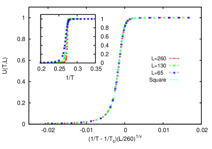
Figure 7: (Color on-line) Result of a Bayesian FSS of the Binder ratio of the Ising model on triangular lattices. We apply the GP regression with Eq. (23). The results of the MC estimate are $1/T_{c}=0.274652(7)$ and $1/\nu=0.989(4)$. The dashed (light-blue) curve is the scaling function of a square lattice in Fig. 3 with a nonuniversal metric factor $C_{1}=1.748(3)$. Inset: Binder ratios of the Ising model on triangular lattices. The number of data items is 86.

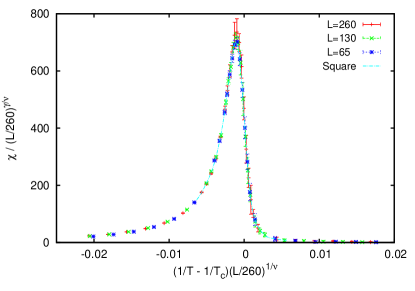
Figure 8: (Color on-line) Result of a Bayesian FSS of the magnetic susceptibility of the Ising model on triangular lattices. We apply the GP regression with Eq. (23) to the data with the same temperatures and lattice sizes of data as in Fig. 7. The results of the MC estimate are $1/T_{c}=0.27466(7)$, $1/\nu=0.95(2)$, and $\gamma/\nu=1.71(2)$. The dashed (light-blue) curve is the scaling function of a square lattice in Fig. 6 with nonuniversal metric factors $C_{1}=1.70(2)$ and $C_{2}=0.777(7)$.

Next, we apply the GP regression to the Binder ratio and magnetic susceptibility on triangular lattices. These results are shown in Fig. 7 and Fig. 8, respectively. All points of each quantity collapse on a curve. The results of the MC estimate for $1/T_{c}$, $1/\nu$, and $\gamma/\nu$ are summarized in Tab. 1. Although they are almost consistent with the exact results, the accuracy of inference is lower than that for the data of square lattices. Since the region of the data of triangular lattices is wide (compare Fig. 7 with Fig. 3), we may consider the correction to scaling.

Table 1: Results of the MC estimates for $1/T_{c}$, $1/\nu$, and $\gamma/\nu$. The exact values of $1/T_{c}$ for square and triangular lattices Onsager (1944); *1952PhRv...85..808Y are $\ln(1+\sqrt{2})/2=0.4406867925\cdots$ and $(\ln 3)/4=0.2746530723\cdots$, respectively. The exact values of $1/\nu$ and $\gamma/\nu$ are $1$ and $\frac{7}{4}$, respectively.

Data	Lattice	Method	$1/T_{c}$	$1/\nu$	$\gamma/\nu$
Binder ratio	Square	GP regression	$0.440683(7)$	$0.996(2)$	-
Binder ratio	Triangular	GP regression	$0.274652(7)$	$0.989(4)$	-
Binder ratio	Square	Least-square	$0.44069(2)$	$1.00(2)$	-
Binder ratio	Square	GP regression	$0.44070(2)$	$1.00(1)$	-
Binder ratio	Square	GP regression	$0.440675(9)$	$0.997(2)$	-
Magnetic susceptibility	Square	GP regression	$0.44072(8)$	$0.98(2)$	$1.74(2)$
Magnetic susceptibility	Triangular	GP regression	$0.27466(7)$	$0.95(2)$	$1.71(2)$

Privman and Fisher proposed the universality of the finite-size scaling function Privman and Fisher (1984). If two critical systems belong to the same universality class, the two finite-size scaling functions with nonuniversal metric factors are equal as

$$\Psi(x)=C_{2}\ \Psi^{\prime}(C_{1}x),$$ (24)

where $\Psi$ and $\Psi^{\prime}$ are finite-size scaling functions and $C_{1}$ and $C_{2}$ are nonuniversal metric factors. Hu et al. checked this idea for bond and site percolation on various latticesHu et al. (1995). The Ising models on square and triangular lattices belong to the same universality. Thus, the two scaling functions must be equal via nonuniversal metric factors as in Eq. (24). To check the universality of finite-size scaling functions, we compared the data on triangular lattices with the scaling function inferred from the data on square lattices. We estimated nonuniversal metric factors to minimize the residual between them. The result for the Binder ratio is $C_{1}=1.748(3)$. The results for the magnetic susceptibility are $C_{1}=1.70(2)$ and $C_{2}=0.777(7)$. Note that there is no metric factor $C_{2}$ for the Binder ratio, because the Binder ratio is dimensionless. The scaling functions of a square lattice with nonuniversal metric factors are shown using the dashed (light-blue) curves in Fig. 7 and Fig. 8. They agree well with the data on triangular lattices. The reduced chi-square of the Binder ratio is $2.65$, and that of magnetic susceptibility is $0.36$. Therefore, we confirm the universality of finite-size scaling functions for the Binder ratio and magnetic susceptibility of the two-dimensional Ising model. We note that Tomita et al. Tomita et al. (1999) confirmed the universality of finite-size scaling functions for other quantities, and Mangazeev et al. Mangazeev et al. (2010) studied the universality of the scaling function in the thermodynamic limit.

IV Conclusions

In this paper, we introduced a Bayesian framework in the scaling analysis of critical phenomena. This framework includes the least-square method for the scaling analysis as a special case. It can be applied to a wide variety of scaling hypotheses, as shown in Eq. (2). In this framework, we proposed the GP regression with GKF defined by Eqs. (10), (14), and (16). This method assumes only the smoothness of a scaling function, and it does not need a form. We demonstrated it for the FSS of the Ising models on square and triangular lattices. For the data limited to a narrow region near a critical point, the accuracy of the GP regression was comparable to that of the least-square method. In addition, for the data to which we cannot apply the least-square method with a polynomial of low degree, our method worked well. Therefore, we confirm the advantage of the GP regression with GKF for the scaling analysis of critical phenomena.

The GP regression can also infer a scaling function as the mean function $\mu$ in Eq. (15). By comparing the data on triangular lattices with the scaling function inferred from the data on square lattices, we confirmed the universality of the FSS function of the two-dimensional Ising model. The use of the scaling function may help in the determination of a universality class.

In this paper, we assume that the data obey a scaling law. However, in some cases, a part of the data may not obey the scaling law. In such a case, we usually introduce a correction to scaling. If we can assume the form of a correction to scaling, we change only the function $Y$ in Eq. (2). However, the assumption of the correction term may cause a problem. In other words, the identification of a critical region remains.

As shown in this paper, the GP regression is a powerful method. In particular, the GP regression can be applied to the statistical check for data collapse. For example, we can apply it to the estimate of nonuniversal metric factors in Fig. 7 and Fig. 8. Another interesting application may be found in the data analysis of physics.