Multi-resonance of energy transport and absence of heat pump in a force-driven lattice

Abstract

Energy transport control in low dimensional nano-scale systems has attracted much attention in recent years. In this paper, we investigate the energy transport properties of Frenkel-Kontorova lattice subject to a periodic driving force, in particular, the resonance behavior of the energy current by varying the external driving frequency. It is discovered that in certain parameter ranges, multiple resonance peaks, instead of a single resonance, emerge. By comparing the nonlinear lattice model with a harmonic chain, we unravel the underlying physical mechanism for such resonance phenomenon. Other parameter dependencies of the resonance behavior are examined as well. Finally, we demonstrate that heat pumping is actually absent in this force-driven model.

I Introduction

In the last decade much attention has been paid to heat conduction on the nanoscale. Numerous studies in the quest of manipulating heat have brought substantial progresses in the area of Phononics, the science and engineering of phonons WL08 . Theoretical models of various thermal devices such as thermal rectifier devices1 , thermal transistor devices2 , thermal logic gates devices3 and thermal memory devices4 have been proposed to control phonon-based thermal transport. In addition, some experimental works have been carried out. For instance, solid-state thermal diodes based on asymmetric nanotube exp_diode1 , asymmetric cobalt oxides exp_diode3 , the nanotube phonon waveguide waveguide and solid thermal memoryXie2011 have been realized experimentally. In the works mentioned above, heat always flows from high temperature region to low temperature one. This is in accordance with the second law of thermodynamics.

However, just like its macroscopic counterpart, a heat pump which directs heat against thermal bias by using external force exists on the molecular level. Recent studies have suggested several such kind of models based on different mechanisms. Li et al. proposed a heat ratchet to direct heat flux from one bath to another in a nonlinear lattice, which periodically adjusts two baths’ temperatures while the average remains equal Li0809 . Later, Ren and Li demonstrated that heat energy can be rectified between two baths of equal temperatures at any instant and the correlation between the baths can even direct energy current against thermal bias without external modulations Ren10 . Beyond those classical models, a quantum heat pump consisting of a molecule connected to two phonon baths was proposed recently Segal0608 , and the Berry phase effect induced heat pump was unraveled as well Ren10PRL .

Nevertheless, some contradiction exists in the force-driven heat pump. Marathe et al showed that under periodic force driving, two coupled oscillators connected with thermal baths fail to function as a heat pump Marathe07 . Later Ai et al claimed the heat pumping appeared in Frenkel-Kontorova (FK) chain under the influence of a periodic driving force Ai2010 . In addition, they observed a thermal resonance phenomenon that the heat flux attained a maximum value at a particular driving frequency, which is similar to the previously found resonance induced by driving bath temperatures Ren10 . However, other than the temperature driven case, a clear physical mechanism of the driving-force-induced resonance is still unavailable.

In this paper, we investigate the force-driven FK chain as a typical nonlinear lattice model and analyze thermal properties which are frequency dependent. We discover that multiple resonance peaks, instead of a single peak, emerge in certain parameter ranges. The origin of this phenomenon in fact relies on the eigenfrequencies of this system. The paper is organized as follows. First of all, we will introduce the FK model and briefly show the crossover from a single resonance to multiple resonances. To look into the underlying mechanism of the multi-resonance phenomenon, we invoke a harmonic model through which analytic expressions of various quantities are obtained. Then the resonance behavior of the FK model is discussed in detail. We will show that as far as the resonance property is concerned, there is much similarity between the FK model and the harmonic model. The effect of different system parameters on the resonance phenomenon is explored as well. In the end, we shall briefly demonstrate that the force-driven model fails to perform as a heat pump.

II Model and Results

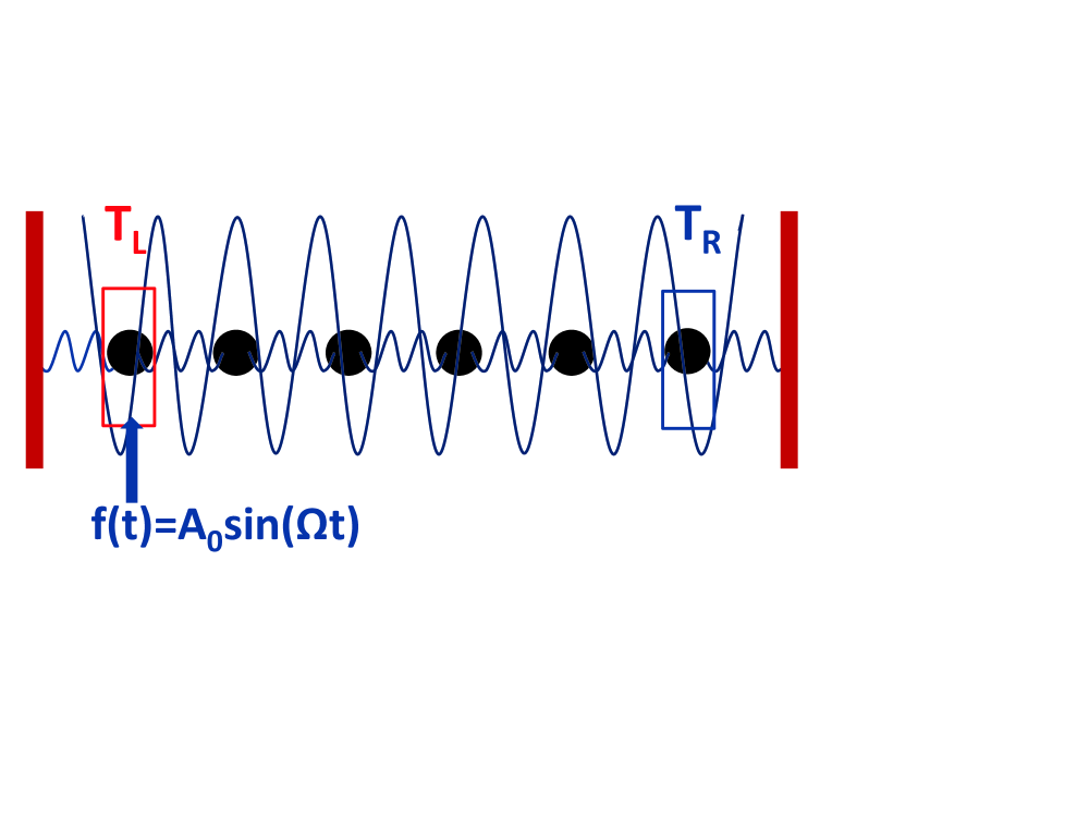
Figure 1: (Color online) Schematic of a one-dimensional FK lattice coupled to two Langevin baths. The left end is attached to a periodic driving force $f(t)$.

We start with a FK chain coupled to Langevin heat baths at two ends. A periodic force is applied to the left end (See Fig. 1). The Hamiltonian of the system is given as:

$$H =\sum^{N}_{i}\frac{p_{i}^{2}}{2m}+\frac{1}{2}k(x_{i}-x_{i+1})^{2}-\frac{V}{(2\pi)^{2}}\cos(\frac{2\pi}{a}x_{i})\qquad$$

$$\ \quad-\delta_{i\alpha}x_{i}f(t),$$ (1)

where $f(t)=A_{0}\sin(\Omega t)$ is the driving force with amplitude $A_{0}$ and frequency $\Omega$ imposed on particle $\alpha$. $x_{i}$ denotes the displacement of the $i$th particle and $p_{i}$ the corresponding momentum. $k$ is the spring constant, $V$ the strength of the on-site potential and $a=1$ the spacing between adjacent particles. We set $\alpha=1$ in follows unless otherwise stated. Under fixed boundary condition, the equation of motion (EOM) of the coupled particles ($i=2,\cdots N-1$) reads:

$$m\ddot{x}_{1} =-\frac{V}{2\pi}\sin(2\pi x_{1})+k(x_{2}-2x_{1})+f(t)\qquad$$ (2a)

$$\qquad-\gamma\dot{x}_{1}\ +\eta_{L}(t),$$

$$m\ddot{x}_{i} =-\frac{V}{2\pi}\sin(2\pi x_{i})+k(x_{i+1}+x_{i-1}-2x_{1}),\quad$$ (2b)

$$m\ddot{x}_{N} =-\frac{V}{2\pi}\sin(2\pi x_{N})+k(x_{N-1}-2x_{N})\qquad$$

$$\qquad-\gamma\dot{x}_{N}\ +\eta_{R}(t).$$ (2c)

The two noise terms are white noise with $\langle\eta_{i}(t)\eta_{j}(t^{\prime})\rangle=2\gamma k_{B}T_{i}\delta_{ij}\delta(t-t^{\prime})$, $(i,j=L,R)$, where $\gamma$ is the friction coefficient, $k_{B}$ is the Boltzmann’s constant and $T_{L(R)}$ denotes the temperature of $L(R)$ reservoir. Without loss of generality, we set $m=1$, $k_{B}=1$ and integrate the EOM by the symplectic Velocity Verlet algorithm. The simulation are performed long enough (of order $10^{8}$) with a time step of $0.005$ to allow the system to reach a non-equilibrium steady state. The local energy current is defined as $I_{i}(t)=\langle-k\dot{x}_{i}(x_{i}-x_{i-1})\rangle$, where $\langle\cdots\rangle$ denotes the ensemble average. After the transient time, the transport approaches an oscillatory steady state and the periodic average of local current is equivalent at each site $i$, reading

$$J_{i}=\frac{\Omega}{2\pi}\int_{0}^{{2\pi}/{\Omega}}I_{i}(t)dt.$$ (3)

There is no doubt that the thermal resonance exists for the energy current as a function of the driving frequency. However, surprisingly, we observe that multiple resonance peaks emerge when the amplitude $A_{0}$ is increased, as shown in Fig. 2. To analyze this multi-resonance phenomenon further, we invoke the harmonic chain model, of which clear analytic results are possible.

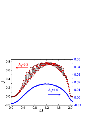
Figure 2: (Color online) Energy current $J$ vs the driving frequency $\Omega$ in the force-driven FK model. Parameters are $T_{L}=0.4,T_{R}=0.6,k=1,V=5,\gamma=1$, and $N=64$. $J$ denotes $J_{i}$ ($i>\alpha=1$). The left arrow means the upper curve corresponds to the left scale while the right arrow means the lower curve corresponds to the right scale. At large $\Omega$, the response of the system cannot catch up with the fast driving as if there is no driving. At small $\Omega$, the system reduces to a quasi-static counterpart as if there is no driving as well. Therefore, at these two regions, $J<0$ since $T_{L}<T_{R}$.

II.1 Analytic results for force-driven harmonic lattice

Harmonic potential is a second order approximation of realistic potential around its minimum. Under harmonic approximation, phonons will not interact with each other. Starting from this noninteracting picture, interactions within phonon gas can be introduced, by including higher order terms in the potential expansion. Compared to non-linear models such as the FK lattice, a harmonic model has the advantage of having an exact solution and it gives many satisfactory explanations about thermal properties of the crystal.

The linear harmonic model considered in this section is obtained by replacing the nonlinear on-site potential in Eq. (II) by $\frac{1}{2}k_{o}x_{i}^{2}$, where $k_{o}$ is the force constant of the on-site harmonic potential. As we shall see, under certain conditions the effect of the driving force can be separated from that of the thermal reservoirs. The EOM in a compact matrix form is:

$$\mathbf{M}\ddot{X}=-\mathbf{\Phi}X-\mathbf{\Gamma}\dot{X}+\eta(t)+F(t),$$ (4)

where $\mathbf{M}$ is the mass matrix set as identity matrix and $\mathbf{\Phi}$ the real symmetric force matrix, with $\Phi_{ij}=(2k+k_{o})\delta_{ij}-k\delta_{i,j+1}-k\delta_{i,j-1}$. $\Gamma_{ij}=\gamma\delta_{ij}(\delta_{i1}+\delta_{iN})$ denotes the coupling to reservoirs. $X=(x_{1},x_{2},\cdots,x_{N})^{T}$ is the vector of displacements and $\eta(t)=(\eta_{L},0,\cdots,0,\eta_{R})^{T}$ depicts the thermal noise in reservoirs. $F(t)$ is a column vector with elements $f_{i}(t)=\delta_{i\alpha}A_{0}\sin(\Omega t)$, denoting the driving force which acts on the $\alpha$th particle. Defining the Fourier transform of quantity $A$ and its inverse:

$$\tilde{A}(\omega)=\frac{1}{2\pi}\int_{-\infty}^{\infty}e^{i\omega t}A(t)dt,\quad{}A(t)=\int_{-\infty}^{\infty}e^{-i\omega t}\tilde{A}(\omega)dw,$$

and applying them to Eq. (4), we obtain

$$X(t) = X^{s}(t)+X^{d}(t),$$ (5)

$$X^{s}(t) = \int_{-\infty}^{\infty}d\omega\,e^{-i\omega t}\mathbf{G}(\omega)\tilde{\eta}(\omega),$$

$$X^{d}(t) = \int_{-\infty}^{\infty}d\omega\,e^{-i\omega t}\mathbf{G}(\omega)\tilde{F}(\omega),$$

where $\mathbf{G}(\omega)=(\mathbf{\Phi}-\omega^{2}\mathbf{M}-i\omega\mathbf{\Gamma})^{-1}$ is the phonon Green’s function. It is clear that the displacement vector $X(t)$ is a superposition of two contributions: $X^{s}$, as the effect of the stochastic heat bath, and $X^{d}$, as the consequence of the driving force. For our periodic driving case, it is easy to get $X^{d}(t)=-\text{Im}[\mathbf{G}(\Omega)\tilde{f}e^{-i\Omega t}]$, with $\tilde{f}_{i}=\delta_{i\alpha}A_{0}$. Similarly, the velocity has the same decomposition $\dot{X}=\dot{X}^{s}+\dot{X}^{d}$, with $\dot{X}^{d}=\text{Im}[i\Omega\mathbf{G}(\Omega)\tilde{f}e^{-i\Omega t}]$. Straightforwardly, following the definition, the local energy current can be similarly expanded as well:

$$I_{i}(t) = I^{s}_{i}(t)+I^{d}_{i}(t)$$ (6)

$$I^{s}_{i}(t) = -k\langle\dot{x}^{s}_{i}(x^{s}_{i}-x^{s}_{i-1})\rangle$$

$$I^{d}_{i}(t) = -k\dot{x}^{d}_{i}(x^{d}_{i}-x^{d}_{i-1}).$$

With $I_{i}(t)$ written in this form, it is obviously that the contributions of noise term and driving force to the energy current are independent from each other. We should note this independence comes from the fact that the driving force is not statistically correlated to the heat baths. Since in the present case, the driving force is deterministic, we have dropped the notation of ensemble average $\langle\cdots\rangle$ in $I^{d}_{i}(t)$.

$I^{s}_{i}(t)$ is just the conventional steady-state heat flux, which is proportional to the temperature difference and is given by $I^{s}_{i}=\frac{\gamma^{2}(T_{L}-T_{R})}{\pi}\int d\omega\,\omega^{2}|G_{1N}(\omega)|^{2}$  Dhar2008 . Thus, the contribution of stochastic heat bath to the oscillatory steady state energy current is just $J^{s}_{i}=\Omega/(2\pi)\int_{0}^{{2\pi}/{\Omega}}I^{s}_{i}dt=I^{s}_{i}$. In all the following discussions and simulations, we will set $\Delta T=T_{L}-T_{R}=0$ unless otherwise stated, since a finite temperature difference mainly causes an additive shift of the energy current curve.

To obtain the expression of $J^{d}_{i}$, we just need to calculate the product of displacement and velocity contributed from the driving force by applying Eq. (5). Denoting $\mathcal{R}(\Omega)\equiv\text{Re}[\mathbf{G}(\Omega)]$ and $\mathcal{I}(\Omega)\equiv\text{Im}[\mathbf{G}(\Omega)]$, we have

$$x^{d}_{i}\dot{x}^{d}_{j}=A_{0}^{2}\Omega[\mathcal{R}_{i\alpha}\mathcal{I}_{j\alpha}\sin^{2}(\Omega t)-\mathcal{I}_{i\alpha}\mathcal{R}_{j\alpha}\cos^{2}(\Omega t)$$

$$+\frac{1}{2}\mathcal{R}_{i\alpha}\mathcal{R}_{j\alpha}\sin(2\Omega t)-\frac{1}{2}\mathcal{I}_{i\alpha}\mathcal{I}_{j\alpha}\sin(2\Omega t)].$$ (7)

Since the driving force is periodic such that the steady state energy current is oscillatory, we take the periodic average of the physical quantities, and the final expression of driving-force-contributed energy current is:

$$J^{d}_{i} =\frac{kA_{0}^{2}\Omega}{2}[\mathcal{R}_{i-1\alpha}(\Omega)\mathcal{I}_{i\alpha}(\Omega)-\mathcal{I}_{i-1\alpha}(\Omega)\mathcal{R}_{i\alpha}(\Omega)]$$

$$=\frac{kA_{0}^{2}\Omega}{2}\text{Im}[{G}^{*}_{i-1\alpha}(\Omega){G}_{i\alpha}(\Omega)].$$ (8)

Therefore, when $T_{1}=T_{2}$, $J_{i}=J^{s}_{i}+J^{d}_{i}=J^{d}_{i}$. In fact, $J^{d}_{i}$ has two values ($i\leqq\alpha$ and $i>\alpha$) and is constant on each side of the driven site $\alpha$. A direct proof is detailed in the Appendix.

From the expression of Eq. (II.1), we should be aware that the energy flux possesses the denominator $D(\Omega)\equiv|\det[\textbf{Z}(\Omega)]|^{2}$ with $\textbf{Z}(\Omega)\equiv\mathbf{\Phi}-\Omega^{2}\mathbf{M}-i\Omega\mathbf{\Gamma}$. Therefore, when $D(\Omega)$ approaches its minimums under certain driving frequencies, the energy flux will exhibit its maximum values. As a consequence, resonance emerges. Let us denote $P_{N}(\Omega)=\det(\mathbf{\Phi}_{N}-\Omega^{2}\mathbf{M})$ to be the characteristic polynomial of the $N\times N$ force matrix $\mathbf{\Phi}_{N}$ with $N$ particles. It can be shown that,

$$\det[\mathbf{Z}(\Omega)]=P_{N}(\Omega)-\gamma^{2}\Omega^{2}P_{N-2}(\Omega)-2i\gamma\Omega P_{N-1}(\Omega),$$ (9)

where $P_{N-1}(\Omega)$ is the characteristic polynomial of the $(N-1)\times(N-1)$ force matrix $\mathbf{\Phi}_{N-1}$ with the first row and column or the last row and column taken out from $\mathbf{\Phi}_{N}$. $P_{N-2}(\Omega)$ is the characteristic polynomial of the $(N-2)\times(N-2)$ force matrix $\mathbf{\Phi}_{N-2}$ with both the first and last rows and columns taken out from $\mathbf{\Phi}_{N}$. Therefore, the denominator $D(\Omega)$ is given by

$$D(\Omega)=[P_{N}(\Omega)-\gamma^{2}\Omega^{2}P_{N-2}(\Omega)]^{2}+4\gamma^{2}\Omega^{2}P_{N-1}^{2}(\Omega).$$ (10)

Apparently, resonant frequencies correspond to those values of $\Omega$ which make $D(\Omega)$ locally minimized. It is difficult to get the explicit exact solutions for those locally minimized solutions. Nevertheless, much simpler and inspiring results can still be obtained if we consider the limiting case with either small friction coefficient or sufficiently large friction. For small friction, we can just set $\gamma=0$ in Eq. (10) and obtain $D(\Omega)=P_{N}^{2}(\Omega)$. Then, the resonant frequencies of the energy current are just the $N$ eigenfrequencies of the force matrix $\mathbf{\Phi}_{N}$. For large friction, by keeping only the highest order terms of $\gamma$ in Eq. (10), we get $D(\Omega)\sim P_{N-2}^{2}(\Omega)$. In this limiting case, the resonant frequencies correspond to the $N-2$ eigenfrequencies of $\mathbf{\Phi}_{N-2}$. When the friction is in between the two cases, we have to minimize $D(\Omega)$ to get those resonant $\Omega$, which should be a gradual shift between the eigenfrequencies of $\mathbf{\Phi}_{N-2}$ and $\mathbf{\Phi}_{N}$.

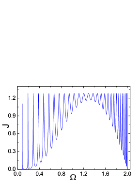
Figure 3: (Color online) Steady state energy current versus driving frequency in the harmonic lattice. $k=1$, $k_{o}=0$, $A_{0}=3.2$, $\gamma=1$, $\Delta T=T_{L}-T_{R}=0$, $N=32$ and $\alpha=1$.

Using Eq. (II.1), we calculate energy current vs driven frequencies, as shown in Fig. 3. It is not surprising to observe the multiple-peak resonance behavior in the harmonic case, since whenever the driven frequency approaches one of the system’s eigenfrequencies, resonance will occur. The number of the eigenfrequencies is mainly determined by the system size.

We can also define other quantities such as the rate of heat released from the two heat baths and rate of work done by the driving force. Their definitions and analytical expressions are given below:

$$\dot{q}_{L}\equiv\langle\dot{x}_{1}(\eta_{L}-\gamma\dot{x}_{1})\rangle=\langle\dot{x}^{s}_{1}(\eta_{L}-\gamma\dot{x}^{s}_{1})\rangle-\gamma(\dot{x}^{d}_{1})^{2},$$ (11)

where $\dot{q}_{L}$ stands for the rate of heat released from the left bath. The first term is contributed by heat baths and is zero when $\Delta T=0$, while the second term comes from the driving force. Therefore the periodic average at $\Delta T=0$ gives

$$\dot{Q}_{L}=\frac{\Omega}{2\pi}\int_{0}^{{2\pi}/{\Omega}}dt\dot{q}_{L}=\dot{Q}^{s}_{L}+\dot{Q}^{d}_{L}=-\frac{\gamma A_{0}^{2}\Omega^{2}}{2}|G_{1\alpha}(\Omega)|^{2}.$$ (12)

Similarly, the expression for $\dot{Q}_{R}$, the average rate of heat released from the right bath, is given as follows

$$\dot{Q}_{R}=\dot{Q}^{s}_{R}+\dot{Q}^{d}_{R}=-\frac{\gamma A_{0}^{2}\Omega^{2}}{2}|G_{N\alpha}|^{2}.$$ (13)

The rate of work done by the driving force is defined as

$$\dot{w}(t)\equiv\langle f(t)\dot{x}_{\alpha}\rangle=f(t)\dot{x}^{d}_{\alpha}$$ (14)

where $f(t)=A_{0}\sin(\Omega t)$. Its periodical average gives

$$\dot{W}=\frac{\Omega}{2\pi}\int_{0}^{{2\pi}/{\Omega}}dt\dot{w}(t)=\frac{A_{0}^{2}\Omega}{2}\mathcal{I}_{\alpha\alpha}(\Omega).$$ (15)

Just like the energy flux, $\dot{W},\ \dot{Q}_{L}$ and $\dot{Q}_{R}$ also show multi-resonance behavior zhangsongNUS . By the continuity equation, the energy current flowing out and into a particle must cancel each other when the system reaches its steady state, since the local energy density does not vary with time at steady state. Therefore, we immediately obtain the relation $\dot{W}+\dot{Q}_{L}=J_{i}=-\dot{Q}_{R}$ ($i>\alpha$), which obeys the energy conservation. For the harmonic model, a direct proof is given in the Appendix. We should also be aware that this relation also holds in the FK model and this is verified by numerical results.

II.2 Multiple resonances of energy transport in force-driven FK model

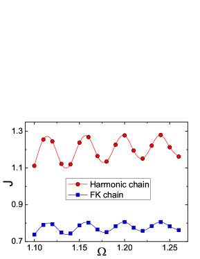
Figure 4: (Color online) Comparison of the FK case and harmonic case with force amplitude $A_{0}=3.2$ in a randomly selected frequency region. Other parameters are $k=1$, $k_{o}=0$, $V=5$, $\gamma=1$, $\Delta T=0$, $N=64$ and $\alpha=1$.

The main qualitative difference between the multiple-resonance curves in Fig. 2 and 3 lies in the fact that the height of the peak for the FK case is smaller than that for the harmonic case, due to the nonlinear on-site potential. This is more obvious for low and high frequency regime. More importantly, we notice that the positions of multiple peaks of the two models seem to be close to each other, as illustrated in Fig. 4. This suggests that the FK model and harmonic model share a similar resonance mechanism. The harmonic model discussed in Sec. II.1 is able to shed lights on the multi-resonance mechanism in a force-driven nonlinear lattice. It is worthwhile to point out that when sampling frequency is not dense enough, one may get a single peak, which actually corresponds to the lower envelope of the multi-resonance curve. When $A_{0}$ decreases, the system seems to have a single peak even though we increase the density of the sampling points, as shown in Fig. 2. The mechanism for the single peak should still be explained by the fact that the driving frequency is resonant with the system’s characteristic frequencies. However, the non-linear potential smooths out the peaks of multi-resonances. In this way, we can only observe the lower envelope so that only one peak is observable. Thus the single-resonance curve does not completely reflect the intrinsic transport property of the FK model.

Let us examine how the parameters of the system will affect the multi-resonance curve. We have already seen the case of the appearance of multiple peaks when $A_{0}$ increases, as shown in Fig. 2. When $A_{0}$ becomes large, the kinetic energy of the particle gained from driving force will be much larger than the height of the on-site potential. In this way, the mask effect of nonlinear on-site potential becomes negligible and the FK model effectively reduces to a harmonic model without on-site potential. This is also demonstrated in Fig. 5 with $A_{0}=10$. We arbitrarily choose three typical regimes of driving frequency: small, moderate and large $\Omega$. In all three regimes, the FK model is very close to the harmonic one. Thus, as long as $A_{0}$ becomes large enough, the mask effect of nonlinearity will fade away and the intrinsic multiple resonant peaks will emerge.

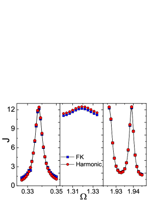
Figure 5: (Color online) Heat current vs driven frequency for large force amplitude $A_{0}=10$. (a) Low frequency regime. (b) Moderate frequency regime. (c) High frequency regime. Other parameters are the same as in Fig. 4.

We are also interested in the effect of temperature. Considering that $T$ (defined as $T\equiv{(T_{L}+T_{R})}/{2}$) will take the role of thermal excitation which mainly affects the kinetic energy of particles, we expect a large value of $T$ will have a similar effect with $A_{0}$ on the resonance behaviors. As shown in Fig. 2 with $T=0.5$ and $A_{0}=1$, there is no multiple resonances behavior. While for the increased temperature case $T=2.0$, there is clearly a peak in a small $\Omega$ range, as shown in Fig. 6(a), which indicates the multiple peaks resonance behavior in the whole frequency range. At low temperature with large amplitude, this is also the case, as illustrated in Fig. 6(b). When $T$ and $A_{0}$ are both small, compared to the nonlinear on-site potential $V$, particles are confined near their equilibrium positions, within the valley of non-linear on-site potential. By Taylor expansion of the potential to the second order, we see that the non-linear potential reduces to a harmonic one, so that the harmonic approximation works. In this case, the lower bound of the phonon band will be raised by $\sqrt{V}$. The phonon band in this case is therefore moved from $0<\Omega<\sqrt{4k}$ to $\sqrt{V}<\Omega<\sqrt{V+4k}$ interface . (Accordingly, the phonon band of the harmonic model is shifted by the on-site potential $k_{o}$ to $\sqrt{k}_{o}<\Omega<\sqrt{k_{o}+4k}$). Energy transport is forbidden outside the frequency region. It is thus expected to see a shift of the energy flux curve to the right while the multi-resonance are still observed, as shown in Fig. 6(c).

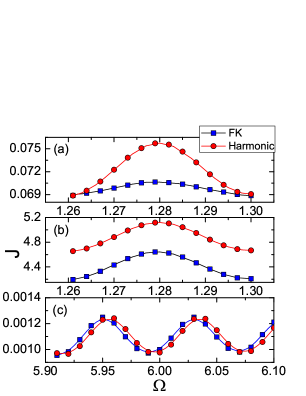
Figure 6: (Color online) Temperature effect on comparison of the FK case and harmonic case. (a) $T=2.0$, $A_{0}=1$. (b) $T=0.01$, $A_{0}=6.4$. (c) $T=0.01$, $A_{0}=0.1$. Other parameters are the same as in Fig. 4, except in (c): $k=10$, $k_{o}=15$ and $V=15$.

The above discussion reveals that there are mainly three dynamic regimes:

(1) When $k_{B}T+{A_{0}a}/({2\pi})\gg{V}/{(2\pi)^{2}}$ ($a$ is the lattice constant as defined previously), the FK model will approach a harmonic model without an on-site potential. Multi-resonances are observable.

(2) For the opposite case, in which $k_{B}T+{A_{0}a}/({2\pi})\ll{V}/{(2\pi)^{2}}$, the FK model reduces to a harmonic model with pure harmonic on-site potential of strength $k_{o}=V$. Multi-resonances are still observable.

(3) When $T+{A_{0}a}/({2\pi})$ is comparable with ${V}/{(2\pi)^{2}}$, the multiple peaks will be smoothed out by the effect of nonlinear on-site potentials and only single resonant peak is observable. In the intermediate regimes, there is the crossover from single peak to multiple peaks, of which the resonant magnitudes are smaller compared with those in the harmonic model.

In addition, the heat released from the baths and the work done by the force in FK model also show parameter-dependent multiple resonances zhangsongNUS , which can be explained by the same mechanism.

III Absence of heat pumping in a force-driven lattice

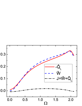
Figure 7: (Color online) $-\dot{Q}_{L}$, $\dot{W}$, $J$ vs the driving frequency in force-driven FK model. Parameters are the same as those for lower single peak curve with $A_{0}=1$, $T_{L}<T_{R}$ in Fig. 2. $\dot{Q}_{L}$ is negative at all frequencies, showing a negative result for pumping effect.

In all simulations so far, we only consider the energy flux flowing into the right reservoir as a whole. In fact it is a sum of two parts: the rate of heat released from the left reservoir into the system and the rate of work done by $f(t)$, i.e, $J=-\dot{Q}_{R}=\dot{Q}_{L}+\dot{W}$. Now let’s consider a typical result of energy transport in a force-driven FK lattice with $T_{L}<T_{R}$, where these two contributions are separated, as shown in Fig. 7. Notably, though $J$ is positive (from $L$ to $R$) in the resonance region, $\dot{Q}_{L}$ is negative in the full range. This indicates heat will always flow into the left reservoir from the chain, whatever the driving frequency is. The corresponding energy flow diagram is depicted in Fig. 8(a). This actually shows that the FK system fails to function as a heat pump since normally, a pump should have an energy flow diagram as in Fig. 8(b), where the heat is absorbed from the low temperature bath and released to the high temperature one. We have tested a broad range of parameters and even in the regimes with multiple resonances. In all cases, the energy never flows as in Fig. 8(b). Therefore we conclude that there is no heat pumping action in a force-driven FK lattice.

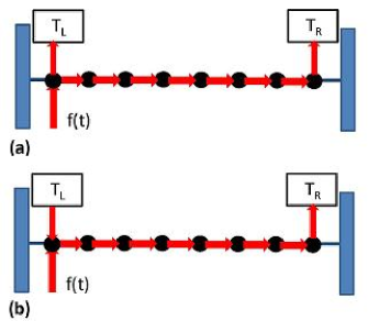
Figure 8: (Color online) (a) A typical energy flow diagram in force-driven FK model with $T_{L}<T_{R}$. (b) The situation when a model performs as a heat pump with $T_{L}<T_{R}$. The arrow denotes the direction of the energy flow.

This finding is consistent with Ref. Marathe07 , wherein it is found that two coupled oscillators of either harmonic or FPU-like interaction would not act as a heat pump under external driving forces. Ref. Ai2010 gets the opposite conclusion, because they overlook the direction of $\dot{Q}_{L}$ and claim the model can act as a heat pump whenever $J$ flows to the right bath of a higher temperature.

To understand the underling mechanism for the absence of heat pumping in a force-driven lattice system, we may consider Eq. (11). The first stochastic contribution is always negative since $T_{L}<T_{R}$. And the second driving contribution, which does not depend on the temperature, always contributes a negative value as well. Thus, $\dot{Q}_{L}$ will still be negative, which indicates the low temperature bath always absorbs rather than releases heat, even we may change the position of the driving force. The situation just corresponds the energy flow diagram in Fig. 8(a).

Clearly as long as the effects of the driving force and the baths are independent, Eq. (11) holds for harmonic chain. Thus for a harmonic system, in order to get a heat pump, a necessary condition is that the driving force is statistically correlated to the bath, such that these two contributions could be synergetic. While in the FK model, effects from the deterministic driving force and stochastic baths are not separable as in Eq. (11) because of the nonlinear on-site potential. However, the nonlinearity can not yet make the two contributions synergetic. And still, our numerical simulations show a negative result for a force-driven FK lattice acting as a heat pump. We thus speculate that for both the force-driven harmonic and nonlinear lattice, the correlation may be the key ingredient for the presence of heat pump action, similar to the entanglement in quantum thermal baths single , the off-equilibrium nonthermal reservoirs Das and the bath noise correlation in temperature-driven case Ren10 , for “low temperature to high temperature” thermal transports.

IV Conclusion

To summarize, we have studied the energy transport control in a force-driven one dimensional nonlinear lattice–the Frenkel-Kontorova model. We have found multiple thermal resonances as a function of the driven frequency. Although not exactly the same, the resonant frequencies are closely related to the eigenfrequencies of the force matrix, and the number of resonant peaks is bounded above by the system size $N$. Moreover, since the onsite nonlinear potential tends to decrease the magnitude of energy current and smoothes out the multiple peaks, the multi-resonance phenomenon is only observable in certain parameter ranges and the crossover from multiple resonances to single resonance will occur. Finally, by following a rigorous definition of heat pump, we clarify a previous contradiction and conclude that heat pumping effect is absent in force-driven lattices.

In this paper, we focus on a one-dimensional chain. However the analysis and results can be generalized to high dimensional system with arbitrary topology, like polymer networks, proteins network1 , and the three dimensional random elastic network network2 , of which the eigen-spectra are much more complicated and non-trivial. The investigation of the resonances in such systems will give us more flexible methods for mechanical control of energy transport in real applications.

V Acknowledgement

This work has been supported in part by an NUS grant, R-144-000-285-646. This work results from Mr. Zhang Song’s “UROPS” (Undergraduate Research Opportunities) project under supervision of Jie Ren and Baowen Li.

APPENDIX

Intuitively, from the energy conservation point of view, the following relations should hold

$$-\dot{Q}_{R} =J_{\alpha+1}=\cdots=J_{N},$$ (16)

$$\dot{Q}_{L} =J_{1}=\cdots=J_{\alpha},$$ (17)

$$\dot{W} =-\dot{Q}_{L}-\dot{Q}_{R}.$$ (18)

However, it is highly nontrivial to give direct proofs for arbitrary nonlinear force-driven lattices. In the following, we will provide a direct proof of the above equations in force-driven harmonic chains by using the analytical forms of $\dot{Q}_{L,R}$, $\dot{W}$ and $J_{i}$.

Let us first define the dimensionless matrix $\mathbf{\hat{Z}}(\Omega)\equiv{\mathbf{Z}(\Omega)}/{k}$, such that ${\hat{Z}}_{ij}=\delta_{i,j}(c-ib\delta_{i,1}-ib\delta_{i,N})-\delta_{i,j+1}-\delta_{i,j-1}$, where $b={\gamma\Omega}/{k}$ and $c=2-{m\Omega^{2}}/{k}$ are two dimensionless parameters. Here we set $k_{o}=0$ without loss of generality. Considering $\mathbf{G}=\mathbf{Z}^{-1}={\mathbf{\hat{Z}}^{-1}}/{k}$, we need a formula for the inversion of the matrix $\hat{\mathbf{Z}}$, which is given in its recurrence form FON :

$$(\mathbf{\hat{Z}}^{-1})_{ij}=\frac{\theta_{i-1}\phi_{j+1}}{\theta_{N}}\quad\text{if }i\leq j,$$ (19)

$$(\mathbf{\hat{Z}}^{-1})_{ij}=\frac{\theta_{j-1}\phi_{i+1}}{\theta_{N}}\quad\text{if }i>j,$$ (20)

where $\theta_{i}$ and $\phi_{i}$ are two sequences, defined by the recurrence relations:

$$\theta_{i} ={\hat{Z}}_{ii}\theta_{i-1}-\theta_{i-2},$$ (21)

$$\phi_{i} ={\hat{Z}}_{ii}\phi_{i+1}-\phi_{i+2},$$ (22)

with the initial condition $\theta_{0}=1$, $\theta_{1}={\hat{Z}}_{11}$, $\phi_{N+1}=1$ and $\phi_{N}={\hat{Z}}_{NN}$. Note $\theta_{N}$ is actually the determinant of the matrix $\mathbf{\hat{Z}}$, which will be denoted as $d$ in follows. Now, to prove Eq. (16), let us recall the expression for $\dot{Q}_{R}$ and $J_{i}$ (see Eq. (II.1) and (13)) and use Eq. (19) and (20). We then get (set $A_{0}=1$ for clearness):

$$-\dot{Q}_{R} =\frac{\gamma\Omega^{2}}{2}|G_{N\alpha}|^{2}=\frac{\gamma\Omega^{2}}{2|d|^{2}k^{2}}|\theta_{\alpha-1}|^{2},$$ (23)

$$J_{i} =\frac{k\Omega}{2}\text{Im}[G_{i-1\alpha}^{*}G_{i\alpha}]$$

$$=\frac{\Omega}{2k|d|^{2}}\text{Im}[(\theta_{\alpha-1}\phi_{i})^{*}(\theta_{\alpha-1}\phi_{i+1})]$$

$$=\frac{\Omega\text{Im}[\phi_{i}^{*}\phi_{i+1}]}{2k|d|^{2}}|\theta_{\alpha-1}|^{2}$$ (24)

where $i>\alpha$. Hence, to prove the above two equations are equivalent with each other, we need to show $\text{Im}[\phi_{i}^{*}\phi_{i+1}]=\gamma\Omega/k$ for all particles to the right of the driving force. We do induction on the index $l$. For $l=N$, the relation is clearly true, which can be taken as the base case. Then suppose the relation is true for all $l\geq i$, we need to show it is also true for $l=i-1$ case. Use the recurrence equation Eq. (21), we have $\text{Im}[\phi_{i-1}^{*}\phi_{i}]=\text{Im}[(c\phi_{i}^{*}-\phi_{i+1}^{*})\phi_{i}]=-\text{Im}[\phi_{i+1}^{*}\phi_{i}]=\text{Im}[\phi_{i}^{*}\phi_{i+1}]=\gamma\Omega/k$. Thus, we have finished the proof that Eq. (16) holds for all particles to the right of the force. A similar proof can be given to show Eq. (17) holds for all particles to the left of the driving force.

Before proceeding to prove Eq. (18), we need more notations. Denote the $n\times n$ matrix $\mathbf{M^{(n)}}$ with elements ${M^{(n)}}_{ij}=c\delta_{i,j}-\delta_{i,j+1}-\delta_{i,j-1}$ and its determinant $K_{n}=det[\mathbf{M}^{(n)}]$, with boundary $K_{-1}=0$ and $K_{0}=1$. The explicit expression of the determinant is given by $K_{n-1}={(y_{1}^{n}-y_{2}^{n})}/{(y_{1}-y_{2})}$, where $y_{1}$, $y_{2}$ is the solution of the quadratic equation $y^{2}-cy+1=0$. We observe that $\theta_{i}$ is in fact the determinant of the sub-matrix in $\mathbf{\hat{Z}}$ starting from the $1st$ row and column to the $ith$ row and column. Similarly $\phi_{i}$ is the determinant of the sub-matrix in $\mathbf{\hat{Z}}$ starting from the $ith$ row and column to the $Nth$ row and column. Now we may expand $\theta_{i}$, $\phi_{i}$ and the determinant of $\mathbf{\hat{Z}}$ in terms of $K_{n}$

$$d =K_{N}-b^{2}K_{N-2}-2ibK_{N-1},$$ (25)

$$\theta_{i} =K_{i}-ibK_{i-1},$$ (26)

$$\phi_{i} =K_{N-i+1}-ibK_{N-i}.$$ (27)

Now we are ready to prove Eq. (18). Let us assume Eq. (18) holds and substitute in the expressions of $\dot{W}$, $\dot{Q}_{L}$ and $\dot{Q}_{R}$ (see Eq. (12), (13) and (15)). Then Eq. (18) becomes $\mathcal{I}_{\alpha\alpha}=\gamma\Omega(|G_{1\alpha}|^{2}+|G_{N\alpha}|^{2})$. With $b={\gamma\Omega}/{k}$ and $G={\mathbf{\hat{Z}}^{-1}}/{k}$, also using Eq. (19)$\sim$ (22), we get

$$\text{Im}(\theta_{\alpha-1}\phi_{\alpha+1}d^{*})=b(|\theta_{\alpha-1}|^{2}+|\phi_{\alpha+1}|^{2}).$$ (28)

Express the left hand side (LHS) and right hand side (RHS) of Eq. (28) in terms of $K_{n}$ (see Eq.($25$)$\sim$($27$)), and after some algebraic work, it can be shown

$$\text{LHS}= b^{3}(K_{\alpha-2}K_{N-2}K_{N-\alpha}+K_{\alpha-1}K_{N-2}K_{N-\alpha-1}$$

$$-2K_{\alpha-2}K_{N-1}K_{N-\alpha-1})$$

$$+b(2K_{\alpha-1}K_{N-1}K_{N-\alpha}-K_{\alpha-2}K_{N}K_{N-\alpha}$$

$$-K_{\alpha-1}K_{N}K_{N-\alpha-1}),$$ (29)

$$\text{RHS}= b^{3}(K_{\alpha-2}^{2}+K_{N-\alpha-1}^{2})+b(K_{\alpha-1}^{2}+K_{N-\alpha}^{2}),$$ (30)

Now in order to show Eq. (18) holds, it is sufficient to prove LHS=RHS to complete the proof. Denote the coefficient of $b^{3}$ ($b$) in LHS by $L_{3}$ ($L_{1}$) and that of RHS by $R_{3}$ ($R_{1}$). By using the formula $K_{n-1}={(y_{1}^{n}-y_{2}^{n})}/{(y_{1}-y_{2})}$ and the fact $y_{1}y_{2}=1$, we get

$$L_{3}= \frac{1}{(y_{1}-y_{2})^{3}}[y_{1}^{2\alpha-1}-y_{2}^{2\alpha-1}+y_{1}^{2N-2\alpha+1}-y_{2}^{2N-2\alpha+1}$$

$$-(y_{1}^{2\alpha-3}-y_{2}^{2\alpha-3})-(y_{1}^{2N-2\alpha-1}-y_{2}^{2N-2\alpha-1})$$

$$-4(y_{1}-y_{2})]=R_{3}.$$ (31)

Note that by a relabeling of $\alpha\rightarrow\alpha+1$ and $N\rightarrow N+2$ in $L_{3}$ and $R_{3}$, and utilizing the relation $K_{n}=cK_{n-1}-K_{n-2}$, we can show $L_{3}\rightarrow L_{1}$ and $R_{3}\rightarrow R_{1}$. Therefore, LHS=RHS and the proof is completed.

References

- (1) L. Wang and B. Li, Phys. World 21, 27 (2008).
- (2) M. Terraneo, M. Peyrard, and G. Casati, Phys. Rev. Lett. 88, 094302 (2002); B. Li, L. Wang, and G. Casati, Phys. Rev. Lett. 93, 184301 (2004).
- (3) B. Li, L. Wang, and G. Casati, Appl. Phys. Lett. 88, 143501 (2006).
- (4) L. Wang and B. Li, Phys. Rev. Lett. 99, 177208 (2007).
- (5) L. Wang and B. Li, Phys. Rev. Lett. 101, 267203 (2008).
- (6) C. W. Chang, D. Okawa, A. Majumdar, and A. Zettl, Science 314, 1121 (2006).
- (7) W. Kobayashi et al Appl. Phys. Lett. 95, 171905 (2009); D Sawaki et al, Appl. Phys. Lett. 98, 081915 (2011)
- (8) C. W. Chang, D. Okawa, H. Garcia, A. Majumdar, and A. Zettl, Phys. Rev. Lett. 99, 045901 (2007).
- (9) R.-G. Xie, C.-T. Bui, B. Varghese, M.-G. Xia, Q.-X. Zhang, C.-H. Sow, B. Li, and J. T. L. Thong, Adv. Funct. Mat 21, 1602 (2011).
- (10) N. Li, P. Hänggi, and B. Li, Europhys. Lett. 84, 40009 (2008); N. Li, F. Zhan, P. Hänggi, and B. Li, Phys. Rev. E 80, 011125 (2009).
- (11) J. Ren and B. Li, Phys. Rev. E 81, 021111 (2010).
- (12) D. Segal and A. Nitzan, Phys. Rev. E 73, 026109 (2006); D. Segal, Phys. Rev. Lett. 101, 260601 (2008).
- (13) J. Ren, P. Hänggi, and B. Li, Phys. Rev. Lett. 104, 170601 (2010).
- (14) R. Marathe, A. M. Jayannavar, and A. Dhar, Phys. Rev. E 75, 030103(R) (2007).
- (15) B. Q. Ai, D. He, and B. Hu, Phys. Rev. E 81 031124 (2010).
- (16) A. Dhar, Adv. Phys. 57, 457 (2008).
- (17) Song Zhang’s “UROPS” project report, Faculty of Science, National University of Singapore, 2010.
- (18) B. Li, J.H. Lan, and L. Wang, Phy. Rev. Lett. 95, 104302 (2005).
- (19) A. E. Allahverdyan and T. M. Nieuwenhuizen, Phys. Rev. Lett. 85, 1799 (2000).
- (20) S. Das, O. Narayan, and S. Ramaswamy, Phys. Rev. E 66, 050103(R) (2002).
- (21) J. Ren and B. Li, Phys. Rev. E 79 051922 (2009).
- (22) H. Hu, A. Strybulevych, J. H. Page, S. E. Skipetrov, and B. A. van Tiggelen, Nature Physics 4, 945 (2008).
- (23) C. M. da Fonseca, J. Comp. Appl. Math. 200, 283 (2007).