Joint and individual variation explained (JIVE) for integrated analysis of multiple data types

Abstract

Research in several fields now requires the analysis of data sets in which multiple high-dimensional types of data are available for a common set of objects. In particular, The Cancer Genome Atlas (TCGA) includes data from several diverse genomic technologies on the same cancerous tumor samples. In this paper we introduce Joint and Individual Variation Explained (JIVE), a general decomposition of variation for the integrated analysis of such data sets. The decomposition consists of three terms: a low-rank approximation capturing joint variation across data types, low-rank approximations for structured variation individual to each data type, and residual noise. JIVE quantifies the amount of joint variation between data types, reduces the dimensionality of the data and provides new directions for the visual exploration of joint and individual structures. The proposed method represents an extension of Principal Component Analysis and has clear advantages over popular two-block methods such as Canonical Correlation Analysis and Partial Least Squares. A JIVE analysis of gene expression and miRNA data on Glioblastoma Multiforme tumor samples reveals gene–miRNA associations and provides better characterization of tumor types.

Data and software are available at https://genome.unc.edu/jive/.

T1Supported in part by NIH Grant R01 MH090936-01, NSF Grant DMS-09-07177, NSF Grant DMS-08-54908 and NIH Grant U24-CA143848.

, , and

1 Introduction

Many fields of scientific research now analyze high-dimensional data, in which a large number of variables are measured for a given set of experimental objects. Increasingly, those data include multiple high-dimensional data sets for a common set of objects. Table 1 gives very diverse examples of such data objects. In this context we refer to each data set as a data type to indicate that it comes from a distinct mode of measurement or domain.

Table 1: Examples with multiple high-dimensional data types

Field	Object	Data types
Computational biology	Tissue samples	Gene expression, microRNA, genotype, protein abundance/activity
Chemometrics	Chemicals	Mass spectra, NMR spectra, atomic composition
Atmospheric sciences	Locations	Temperature, humidity, particle concentrations over time
Internet traffic	Websites	Word frequencies, visitor demographics, linked pages

The motivation for this article is a particular application to biological data. In biomedical studies, a number of technologies now commonly collect diverse information on an organism or tissue sample. The amount of available biological data from multiple platforms and technologies is expanding rapidly. The 2011 Online Database collection of Nucleic Acids Research lists 1330 publicly available databases that measure various aspects of molecular and cell biology [Galberin and Cochrane (2011)]. Large online databases such as ArrayExpress [Parkinson et al. (2009)] and the UCSC Genome-browser [Rhead et al. (2010)] often contain multiple data types collected from a common set of samples. Large-scale projects like The Human Connectome Project [Sporns, Tononi and Kötter (2005)] and The Cancer Genome Atlas [Cancer Genome Atlas Research Network (2008)] focus on the integrated analysis of multiple data types.

Well-established multivariate methods can be used to separately analyze different data types measured on the same set of objects. However, individual analyses will not capture the critical associations and potential causal relationships between data types. Furthermore, each data type can impart unique and useful information. There is a strong need for new statistical methods that explore associations between multiple data types and combine data from multiple sources when making inference about the objects. This motivates an interesting new area of statistical research.

1.1 Data

We describe an application to data from TCGA, an ongoing collaborative effort funded by the National Cancer Institute (NCI) and the National Human Genome Research Institute (NHGRI). A goal of TCGA is to characterize cancer on a molecular level through the analysis and integration of multidimensional large scale genomic data. The integration of information from disparate genomic sources has the promise to provide a more comprehensive understanding of cancer genetics and cell biology.

We focus, in particular, on a set of 234 Glioblastoma Multiforme (GBM) tumor samples. GBM is a common and very fatal form of malignant brain tumor. However, GBM cases are not homogeneous, and an understanding of systematic distinctions between the tumor samples may lead to more targeted therapies. Verhaak et al. (2010) classified the TCGA GBM samples into four subtypes: Neural, Mesenchymal, Proneural and Classical. These subtypes have distinct expression characteristics, copy number alterations and gene mutations. In addition, there were clinical differences across subtypes in response to aggressive therapy.

Copy number aberrations and somatic mutations, and their relation to gene expression, have been recognized as important aspects of GBM biology [see, e.g., Bredel et al. (2009) and Cancer Genome Atlas Research Network (2008)]. However, the role of microRNA (miRNA) data in GBM biology has not been well studied. In this article we focus on the integrated analysis of miRNA and gene expression data. These data are two distinct data types, as they are measured on different platforms and represent different biological components.

Current biological ideas suggest that miRNAs function primarily as post-transcriptional regulators of gene expression. Typically, they are considered negative regulators, decreasing gene expression levels. Many of the algorithms that predict miRNA targets (TargetScan, miRanda, Pictar, and RNA22) have vastly different predicted gene lists [Peter (2010)]. Therefore, miRNA and gene expression relations are not well understood. However, recent research suggests that miRNAs may be partly responsible for the expression of well-known tumor activating genes (oncogenes) and tumor suppressing genes.

Investigating each data type individually would lose some important relations, considering the inherent interactions between miRNAs and gene expression. An integrative, multivariate approach is desired. The data decomposition proposed in Section 1.2 gives new insight into the joint and individual variation between the miRNA and gene expression data. Although this decomposition is unsupervised with respect to the above GBM subtypes, we further investigate how it leads to a better characterization of these subtypes.

For each tumor sample, there are measures of intensity for 534 miRNAs and 23,293 genes (messenger RNA). These data are publicly available from TCGA. The preprocessed data used for this analysis are available at https://genome.unc.edu/jive.

1.2 Proposed method

Given the biological relation between gene expression and miRNA, it is reasonable to expect shared patterns in the two sets of measurements. We refer to such shared patterns as joint structure. We also expect the gene expression data to have systematic variation that is unrelated to the miRNAs and vice versa. This individual structure can be the result of technical artifacts, but may also be of biological interest. For example, miRNA regulation is just one of many factors that can influence gene expression. This structured individual variation can interfere with finding the important joint signal, just as joint structure can obscure the important signal that is individual to a data type.

To separate joint and individual effects, we introduce a method called Joint and Individual Variation Explained (JIVE). This exploratory method decomposes a data set into a sum of three terms: a low-rank approximation capturing joint structure between data types, low-rank approximations capturing structure individual to each data type and residual noise. Analysis of individual structure provides a way to identify potentially useful information that exists in one data type, but not others. Accounting for individual structure also allows for more accurate estimation of what is common between data types. As illustrated in Section 4.2, JIVE can identify joint structure not found by existing methods. It may be used regardless of whether the dimension of a data set exceeds the sample size. Furthermore, JIVE is applicable to data sets with more than two data types and has a simple algebraic interpretation.

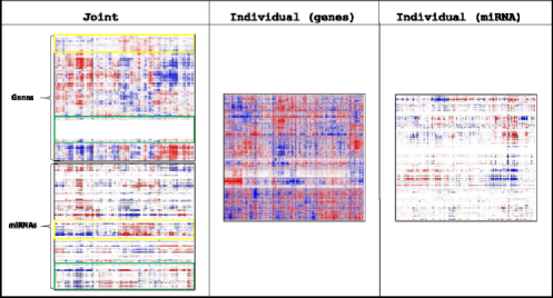
A heatmap of joint structure and individual structure in the GBM data, identified by JIVE, is shown in Figure 1. Columns (corresponding to the 234 samples) are shown in the same order for both gene and miRNA data in the display of joint structure. This common ordering shows complex structure in both data types, and shared patterns are present in subsets of genes and miRNAs. JIVE also identifies a large amount of structured variation individual to the gene expression data and a lesser degree of individual structure in the miRNA data. While the individual structure accounts for more variability in the data than the joint structure, our analysis suggests that the joint structure is more relevant to the cancer biology.

Figure 1: JIVE estimates for joint structure and individual structure in the GBM data. Blue corresponds to negative values, red positive values. Columns are given in the same order in the joint structure, and subsets of genes and miRNAs that share similar patterns are highlighted in green and yellow.

2 Model and estimation

2.1 Formal framework

Formally, we focus on data for multiple matrices $X_{1},X_{2},\ldots,X_{k}$ with $k\geq 2$. Each matrix has $n$ columns, corresponding to a common set of $n$ objects. The $i$th matrix $X_{i}$ has $p_{i}$ rows, each corresponding to a variable in a given measurement technology that varies from matrix to matrix. For example, in our application to GBM data the rows of $X_{1}$ contain gene expression measurements (of dimension $p_{1}=23\mbox{,}293$) and the rows of $X_{2}$ contain miRNA measurements (of dimension $p_{2}=534$) for the same set of 234 tissue samples ($n=234$). The $k$ matrices may be combined into a single data matrix

$$X=\left[\matrix{X_{1}\vspace*{2pt}\cr\vdots\vspace*{2pt}\cr X_{k}}\right]\dvtx p\times n,$$

where $p=p_{1}+p_{2}+\cdots+p_{k}$.

Direct analysis of $X$ can be problematic as the size and scale of the constituent data types often differ. To remove baseline differences between data types, it is helpful to row-center the data by subtracting the mean within each row. Data types may also be of different dimension ($p_{i}$) or differ in variability. To circumvent cases where “the largest data set wins,” it is helpful to scale each data type by its total variation, or sum-of-squares. In particular, for each $i$ define $X_{i}^{\mathrm{scaled}}$ = $\frac{X_{i}}{\|X_{i}\|}$, where $\|\cdot\|$ defines the Frobenius norm $\|A\|^{2}=\sum_{i,j}a_{ij}^{2}$. Then, $\|X_{i}^{\mathrm{scaled}}\|=1$ for each $i$, and each data type contributes equally to the total variation of the concatenated matrix

$$X^{\mathrm{scaled}}=\left[\matrix{X_{1}^{\mathrm{scaled}}\vspace*{2pt}\cr\vdots\vspace*{2pt}\cr X_{k}^{\mathrm{scaled}}}\right].$$ (1)

2.2 Model

Let $X_{1},X_{2},\ldots,X_{k}$ be matrices as in Section 2.1, scaled appropriately. Joint structure is represented by a single $p\times n$ matrix of rank $r<\operatorname{rank}(X)$. Individual structure for each $X_{i}$ is represented by a $p_{i}\times n$ matrix of rank $r_{i}<\operatorname{rank}(X_{i})$.

More formally, let $A_{i}$ be the matrix representing the individual structure of $X_{i}$, and let $J_{i}$ be the submatrix of the joint structure matrix that is associated with $X_{i}$. Then, the unified JIVE model is

$$X_{1} = J_{1}+A_{1}+\varepsilon_{1},$$ (2)

$$\vdots$$

$$X_{k} = J_{k}+A_{k}+\varepsilon_{k},$$

where $\varepsilon_{i}$ are $p_{i}\times n$ error matrices of independent entries with $\mathbb{E}(\varepsilon_{i})=0_{p_{i}\times n}$. Let

$$J=\left[\matrix{J_{1}\vspace*{2pt}\cr\vdots\vspace*{2pt}\cr J_{k}}\right]$$

denote the joint structure matrix. The model imposes the rank constraints $\operatorname{rank}(J)=r$ and $\operatorname{rank}(A_{i})=r_{i}$ for $i=1,\ldots,k$. Furthermore, we require that the rows of joint and individual structures are orthogonal: $JA_{i}^{T}=0_{p\times p_{i}}$ for $i=1,\ldots,k$. Intuitively, this means that sample patterns responsible for joint structure between data types are unrelated to sample patterns responsible for individual structure. This requirement does not constrain the model, in that any matrix in the form (2) can be written equivalently with orthogonality between joint and individual structures. Furthermore, the orthogonality constraint assures that the joint and individual components in (2) are uniquely determined (see the supplementary material [Lock et al. (2012)] for more details). It is remarkable that no further orthogonality constraints (say, between the column space of $J_{i}$ and the column space of $A_{i}$, or between the row spaces of each $A_{i}$) are required to make the decomposition identifiable.

2.3 Estimation

Here we discuss estimation of the model for fixed ranks $r,r_{1},\ldots,r_{k}$. The choice of these ranks is important to accurately quantify the amount of joint and individual structures. The supplementary material [Lock et al. (2012)] describes a permutation testing approach to rank selection.

Joint and individual structures are estimated by minimizing the sum of squared error. Let $R$ be the $p\times n$ matrix of residuals after accounting for joint and individual structures:

$$R=\left[\matrix{R_{1}\vspace*{2pt}\cr\vdots\vspace*{2pt}\cr R_{k}}\right]=\left[\matrix{X_{1}-J_{1}-A_{1}\vspace*{2pt}\cr\vdots\vspace*{2pt}\cr X_{k}-J_{k}-A_{k}}\right].$$

We estimate the matrices $J$ and $A_{1},\ldots,A_{k}$ by minimizing $\|R\|^{2}$ under the given ranks. This is accomplished by iteratively estimating joint and individual structures:

• Given $J$, find $A_{1},\ldots,A_{k}$ to minimize $\|R\|$.

• Given $A_{1},\ldots,A_{k}$, find $J$ to minimize $\|R\|$.

• Repeat until convergence.

The joint structure $J$ minimizing $\|R\|$ is equal to the first $r$ terms in the singular value decomposition (SVD) of X with individual structure removed. The estimated individual structure for $X_{i}$ is equal to the first $r_{i}$ terms of the SVD of $X_{i}$ with the joint structure removed. The estimate of individual structure for $X_{i}$ will not change those for $X_{j}$, $j\neq i$ and, hence, the $k$ individual approximations minimize $\|R\|$ for fixed joint structure. Pseudocode for this iterative algorithm is given in the supplementary material [Lock et al. (2012)]. Computing time can be improved by reducing the dimensionality of $X_{1},\ldots,X_{k}$ at the outset via their SVD (see the supplementary material [Lock et al. (2012)]).

Figure 2: $X$ and $Y$ are generated by adding together joint structure, individual structure and noise. Blue corresponds to negative values, red positive values.

The iterative method is monotone in the sense that $\|R\|$ decreases at each step. Thus, $\|R\|$ converges to a coordinate-wise minimum, which can not be improved by changing the estimated joint or individual, structure. Further convergence properties of the algorithm are currently under study.

2.4 Illustrative example

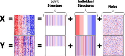
As a basic illustration we generate two matrices, $X$ and $Y$, with simple patterns corresponding to joint and individual structures. The simulated data are depicted in Figure 2. Both $X$ and $Y$ are of dimension $50\times 100$, that is, each has 50 variables measured for the same 100 objects. A common pattern $V$ of 100 independent standard normal variables is added to half of the rows in $X$ and half of the rows in $Y$. This represents the joint structure between the two data sets. Structure individual to $X$ is generated by partitioning the objects into five groups, each of size twenty. Those columns corresponding to group 1, 2, 3, 4 or 5 have $-2$, $-1$, 0, 1, 2 added to each row of $X$, respectively. Structure individual to $Y$ is generated similarly, but the groups are randomly determined and are therefore independent of the groups in $X$. Finally, independent $N(0,1)$ noise is added to both $X$ and $Y$. Note that the important joint structure is visually obscured.

The common pattern $V$ represents an underlying phenomenon that contributes to several variables in both $X$ and $Y$. Practically, the individual structure in $X$ (or $Y$) may correspond to an experimental grouping of the measured variables in $X$ ($Y$) not present in $Y$ ($X$), for example, batch effects in microarray data. Our goal is to identify both the common underlying phenomenon and individual group effects.

Figure 3 shows the JIVE estimate for joint structure, JIVE estimates for individual structure and the fit given by the sum of joint and individual structures. Estimates closely resemble the true signal in Figure 2.

Figure 3: JIVE estimates for joint structure and individual structure. Blue corresponds to negative values, red positive values.

2.5 GBM data

As the gene expression and miRNA data for the GBM samples differ in dimension and variability, they were scaled as in Section 2.1. Permutation testing (see the supplementary material [Lock et al. (2012)]) was used to determine the ranks of estimated joint and individual structures. The test (using $\alpha=0.01$, and 1000 permutations) identified:

• rank 5 joint structure

• rank 33 structure individual to gene expression

• rank 13 structure individual to miRNA.

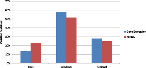
The percentage of variation (sum of squares) explained in each data set by joint structure, individual structure and residual noise is shown in Figure 4. This illustrates how the JIVE decomposition can be used to quantify and compare the amount of shared and individual variation between data types. As shown in Figure 4, joint structure is responsible for more variation in miRNA than in gene expression (23% and 14%, resp.), and the gene expression data has a considerable amount of structured variation (58%) that is unrelated to miRNA. This is consistent with current biological understanding, as miRNAs are just one of several factors that can influence gene expression.

Figure 4: Percentage of variation (sum of squares) explained by estimated joint structure, individual structure and residual noise for miRNA and gene expression data.

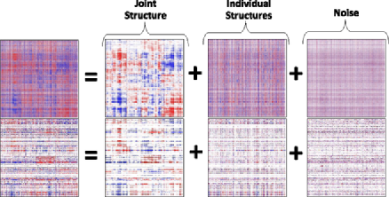
Heatmaps of the low-rank estimates for joint structure, individual structure and residual noise are shown in Figure 5. Columns have the same order in all heatmaps. This reveals the shared patterns present in the joint structure from Figure 1, but little of the structure that is present in the individual estimates.

Figure 5: Heatmaps of low-rank estimates for joint structure, individual structure and residual noise in the gene expression (top) and miRNA (bottom) data. Blue corresponds to negative values, red positive values. Columns have the same order in all heatmaps.

3 Model factorization

3.1 Relation to PCA

The JIVE model can be factorized as in Principal Component Analysis (PCA). For a row-centered $p\times n$ matrix $X$, the first $r$ principal components yield the rank $r$ approximation

$$X\approx US,$$

where $S(r\times n)$ contains the sample scores and $U(p\times r)$ contains the variable loadings for the first $r$ components.

As in PCA, the rank $r$ joint structure matrix $J$ in the JIVE model can be written as $US$, where $U$ is a $p\times r$ loading matrix and $S$ is an $r\times n$ score matrix. Let

$$U=\left[\matrix{U_{1}\vspace*{2pt}\cr\vdots\vspace*{2pt}\cr U_{k}}\right],$$

where $U_{i}$ gives the loadings of the joint structure corresponding to the rows of $X_{i}$. The rank $r_{i}$ individual structure matrix $A_{i}$ for $X_{i}$ can be written as $W_{i}S_{i}$, where $W_{i}$ is a $p_{i}\times r_{i}$ loading matrix and $S_{i}$ is an $r_{i}\times n$ score matrix. Then, the low-rank decomposition of $X_{i}$ into joint and individual structures is given by $X_{i}\approx U_{i}S+W_{i}S_{i}.$ This gives the factorized model

$$X_{1} = U_{1}S+W_{1}S_{1}+R_{1},$$ (3)

$$\vdots$$

$$X_{k} = U_{k}S+W_{k}S_{k}+R_{k}.$$

Joint structure is represented by the common score matrix $S$. These scores summarize patterns in the samples that explain variability across multiple data types. The loading matrices $U_{i}$ indicate how these joint scores are expressed in the rows (variables) of data type $i$. The score matrices $S_{i}$ summarize sample patterns individual to data type $i$, with variable loadings $W_{i}$.

3.2 GBM data

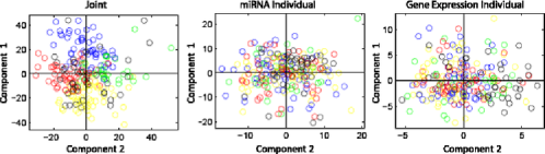
Sample scores for joint structure, matrix $S$ in equation (3), reveal sample patterns that are present across the miRNA and gene expression data. Sample scores for individual structure, matrices $S_{1}$ and $S_{2}$ in equation (3), reveal sample patterns that are individual to each data type. Figure 6 shows separate scatterplots of the sample scores for the first two principal components of estimated joint structure, the first two components individual to miRNA, and the first two components individual to gene expression. Subtype distinctions are clearly present in the scatterplot of joint scores, but a subtype effect is not visually apparent in either of the individual scatterplots.

Figure 6: Scatterplots of sample scores for the first two joint components, first two individual miRNA components and first two individual gene expression components. Samples are colored by subtype: Mesenchymal (yellow), Proneural (blue), Neural (green) and Classical (red). Samples colored black were assayed after the initial subtype analysis and are considered unclassified.

Table 2: SWISS scores for TCGA subtypes. Lower scores indicate more subtype distinction

Data	Gene expression	0.8431
	miRNA	0.8763
JIVE	Joint	0.7678
	Gene expression individual	0.9019
	miRNA individual	0.9284

Since the subtypes are defined by gene expression clustering, their appearance in Figure 6 is not surprising. However, the clustering apparent in the joint plot shows involvement of miRNA in the differentiation of these subtypes. It is interesting that a subtype effect is not apparent in either scatterplot for individual structure, suggesting that this variation is driven by other biological components. This is remarkable, as the fraction of gene expression variation explained by joint structure (see Figure 4) is small.

To numerically compare the extent to which subtype distinctions are present, we consider the standardized within-subtype sum of squares

$$\operatorname{SWISS}(A)=\frac{\sum_{i}\sum_{j}(A_{ij}-\bar{A}_{i,s(j)})^{2}}{\sum_{i}\sum_{j}(A_{ij}-\bar{A}_{i\cdot})^{2}},$$

where $s(j)=\{k\dvtx\mathrm{samples}\ j\mbox{ and }k\mbox{ belong to the same subtype}\}$. This represents the variability within subtypes (across all rows) as a proportion of total variability. Table 2 gives SWISS scores for the gene expression and miRNA data, and SWISS scores for the JIVE estimates of joint and individual structures. A permutation test described in Cabanski et al. (2010) concludes that the four subtypes are significantly more distinguished on the estimated joint structure than on the gene expression and miRNA data ($p<0.001$; $10\mbox{,}000$ permutations). SWISS scores for individual structure in gene expression and miRNA are close to one, as subtype distinctions are almost entirely represented in the joint structure between the two data types. This suggests that miRNA may play a greater role in GBM biology than previously thought.

In general, these analyses illustrate how an unsupervised, integrated analysis across multiple data types can result in a better distinction between subtypes or other biological classes. One could conduct a similar analysis to investigate how the JIVE components relate to survival or other clinical factors, rather than subtype. Furthermore, a direct cluster analysis on the JIVE components could be used to identify sample groups that are distinguished across multiple data types.

4 Comparison with existing methods

4.1 Existing methods

One approach to the analysis of multiple data sets is to mine the data for variable-by-variable associations. In computational biology, large-scale correlation studies can identify millions of pairwise variable associations between genomic data types [see, e.g., Gilad, Rifkin and Pritchard (2008)]. Furthermore, network models can link associated variables across and within data types [see Adourian et al. (2008)]. However, analysis of variable-by-variable associations alone does not identify the global modes of variation that drive associations across and within data types, which is the focus of this paper.

PCA of the block-scaled matrix $X^{\mathrm{scaled}}$ in (1) coincides with Consensus PCA [Wold, Kettaneh and Tjessem (1996), Westerhuis, Kourti and MacGregor (1998)]. This direct approach is also used by the iCluster method [Shen, Olshen and Ladanyi (2009)], which performs clustering based on a factor analysis of the concatenated matrix $X$. While these methods synthesize information from multiple data types, they do not distinguish between joint or individual effects.

Canonical Correlation Analysis (CCA) [Hotelling (1936)] is a popular method to globally examine the relation between two sets of variables. If $X_{1}$ and $X_{2}$ are two data sets on a common set of samples, the first pair of canonical loadings (variable weights) $u_{1}$ and $u_{2}$ are unit vectors maximizing $\operatorname{Corr}(u_{1}^{T}X_{1},u_{2}^{T}X_{2})$. Geometrically, $u_{1}$ and $u_{2}$ can be interpreted as the pair of directions that maximize the correlation between $X_{1}$ and $X_{2}$. Sample projections on the canonical loadings, $u_{1}^{T}X_{1}$ and $u_{2}^{T}X_{2}$, give the canonical scores for $X_{1}$ and $X_{2}$. Subsequent CCA directions can be found by enforcing orthogonality with previous directions. For data sets with $p_{1}>n$ or $p_{2}>n$ the CCA directions are not well defined, and overfitting is often a problem even when $p_{1},p_{2}<n$. Hence, standard CCA is typically not applicable to high-dimensional data.

Partial Least Squares (PLS) [Wold (1985)] directions are defined similarly to CCA, but maximize covariance rather than correlation. PLS is appropriate for high-dimensional data. However, Trygg and Wold (2003) examine how structured variation in $X_{1}$ not associated with $X_{2}$ (and vice versa) can drastically alter PLS scores, making the interpretation of such scores problematic. Their solution, called O2-PLS, seeks to remove structured variation in $X_{1}$ not linearly related to $X_{2}$ (and vice versa) from the PLS components. As such, O2-PLS components are often more representative of the true joint structure between two data types. However, the restriction of O2-PLS (and PLS) to pairwise comparisons limits their utilty in finding common structure among more than two data types.

Witten and Tibshirani (2009) recently introduced Multiple Canonical Correlation Analysis (mCCA) to explore associations and common structure on two or more data sets. For $X_{1},X_{2},\ldots,X_{k}$ as in Section 2.1, standardized so that each row has mean 0 and standard deviation 1, the standard mCCA loading vectors $u_{1},u_{2},\ldots,u_{k}$ satisfy

$$\mathop{\arg\max}_{\|u_{1}\|=\cdots=\|u_{k}\|=1}\sum_{i<j}u_{i}^{T}X_{i}X_{j}^{T}u_{j}=\sum_{i<j}\operatorname{Cov}\bigl{(}u_{i}^{T}X_{i},u_{j}^{T}X_{j}\bigr{)}.$$

As such, mCCA can be viewed as a natural extension of PLS to more than two data types.

Di et al. (2009) develop multi-level functional PCA (MF-PCA) for the analysis of variation between and within grouped samples of functional data. Similar in spirit to JIVE, MF-PCA yields a sum of two PCA decompositions: one for variability between groups and one for variability within groups. We stress that JIVE is designed for analysis across disparate data types, while MF-PCA analyzes grouped observations on the same functional data type. More substantively, MF-PCA does not model shared structure and individual structure. Rather, MF-PCA models structure among main effects (e.g., at the group level) and structured variation about those main effects (e.g., at the sample level), in the context of functional data.

4.2 Illustrative example

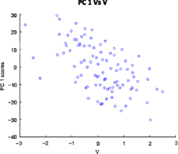
We return to the example introduced in Section 2.4. Consensus PCA of the concatenated matrix $[{X^{\prime}\enskip Y^{\prime}}]^{\prime}$ does a poor job of finding the joint structure. The scatterplot in Figure 7 shows a weak association between the first principal component scores and the joint response $V$. This is because PCA of the concatenated data is driven by all variation in the data, joint or individual.

Figure 8 shows an analysis of PLS and CCA for $X$ and $Y$. The scores for the first PLS direction for $X$ and $Y$ show a weak association (panel C). Furthermore, the PLS scores are not strongly related to the joint response $V$ (panels A and B). Scores for $X$ and $Y$ show a stronger association with $V$ within groups, indicating how for PLS individual structure can interfere with the identification of joint structure. The CCA scores are very highly correlated (panel F), but show nearly no association with the joint or individual structures (panels D and E). This illustrates the tendency of CCA to overfit on high-dimensional data.

Figure 7: Scatterplot of the first consensus principal component scores vs the joint signal $V$. The scores are weakly associated with the joint signal.

Figure 8: Scores for the first PLS, and CCA, directions for $X$ and $Y$. Panels (A) and (B) show some association between the PLS scores and the joint signal $V$. Points are colored by simulated group in both $X$ and $Y$, and are more highly associated with $V$ within each group. The two PLS directions have a weak correlation (C). The CCA directions correlate with each other (F), but not the common signal $V$ (D and E). This illustrates the tendency of CCA to overfit.

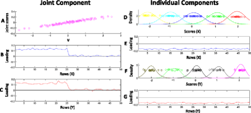
Next we consider the JIVE analysis of $X$ and $Y$. Scores and loadings for the joint component and both individual components are shown in Figure 9. JIVE is able to find the true joint signal between the two data sets, as joint scores are closely associated with the common response $V$ (panel A). Furthermore, individual scores do a good job of distinguishing the groups specific to $X$ and $Y$ (panels D and F). The joint signal was added to only the first 25 variables in $X$ and $Y$, which is reflected in the joint loadings (panels B and C). The individual groups were defined on all 50 variables for both $X$ and $Y$, which is reflected in the individual loadings (panels E and G). Note that joint and individual loadings are not constrained to be orthogonal, which gives the analysis more flexibility.

Figure 9: Scores and loadings for joint and individual components in the JIVE decomposition. Joint scores are highly associated with the common signal $V$ (panel A). Individual scores distinguish groups specific to $X$ and $Y$ (D and F). Joint loadings (B and C) show a strong effect (difference from zero) on half of the variables in $X$ and $Y$. Individual loadings (E and G) show a similar effect on all variables in $X$ and $Y$.

5 Variable sparsity

In many practical applications, important structure between samples or objects is present on only a small subset of the measured variables. This motivates the use of sparse methods, in which only a subset of variables contribute to a fitted model. Sparse versions of exploratory methods such as PCA [Shen and Huang (2008)], PLS [Lê Cao et al. (2008)] and CCA [Parkhomenko, Tritchler and Beyene (2009)] already exist.

Here, we describe the use of a penalty term to induce variable sparsity in the JIVE decomposition. Sparsity is accomplished if some of the variable loadings for joint and individual structures [$U$ and $W_{i}$ in equation (3)] are exactly 0. For weights $\lambda$ and $\lambda_{i}$, we minimize the penalized sum of squares

$$\|R\|^{2}+\lambda\operatorname{Pen}(U)+{\sum}_{i}\lambda_{i}\operatorname{Pen}(W_{i}),$$

where $\operatorname{Pen}$ is a penalty designed to induce sparsity in the loading vectors. In our implementation, $\operatorname{Pen}$ is an $L1$ penalty analogous to Lasso regression [Tibshirani (1996)], namely,

$$\operatorname{Pen}(A)={\sum}_{i,j}|a_{ij}|.$$

Under this penalty, loadings of variables with a small or insignificant contribution tend to shrink to 0. Other sparsity-inducing penalties (e.g., hard thresholding) may be substituted for $L1$ penalization.

Figure 10: Plot of gene–miRNA correlations (A), and scores and loadings for the first two sparse joint components (B–E). In (A), gene–miRNA pairs are colored red if they have a significant positive correlation and blue if they have a signficant negative correlation ($P<10^{-5}$). Panels (B) and (D) show sample scores for the first two joint components, colored by subtype. Panels (C) and (E) display gene–miRNA pairs where both have nonzero loadings. Pairs are colored red if both gene and miRNA loadings have the same sign, blue otherwise. In panels (A), (C) and (E) genes and miRNAs are ordered separately by average linkage correlation clustering.

Estimation with sparsity is accomplished by an iterative procedure analogous to that used for the nonsparse case:

• Given $J$, find $A_{i}$ to minimize $\|R_{i}\|^{2}+\lambda_{i}\operatorname{Pen}(W_{i})$ for each $i=1,\ldots,k$.

• Given $A_{1},\ldots,A_{k}$, find $J$ to minimize $\|R\|^{2}+\lambda\operatorname{Pen}(U)$.

• Repeat until convergence.

At each iteration, the sparsity penalty is incorporated through the use of a sparse singular value decomposition (SSVD), adapted from Lee et al. (2010). The weights $\lambda$, $\lambda_{i}$ may be pre-specified or estimated via the Bayesian Information Criterion (BIC) [Schwarz (1978)] at each iteration.

Inducing sparsity in the joint structure effectively identifies subsets of variables within each data type that are associated. Examination of the joint sample scores, in turn, reveals sample patterns that drive these associations.

5.1 GBM data

A natural way to explore associations between individual genes and miRNAs is to compute the matrix of all gene–miRNA correlations, and then examine the set of significant correlations. Panel A of Figure 10 shows a heatmap of the significant gene–miRNA correlations.

A sparse implementation of JIVE provides an alternative approach to identifying gene–miRNA associations, and can reveal additional structure. Panel B shows the sample scores in the first joint component resulting from a sparse JIVE analysis of the data. Panel C shows all the gene–miRNA pairs with the property that both that gene and miRNA have nonzero loadings in the first joint component. Thus, the nonzero entries of the heatmap have the form of a Cartesian product. We note that the nonzero entries in panel C closely match those in the correlation map of panel A, and that the signs of these entries also show good agreement. Scores for the first joint component (panel B) distinguish the Mesenchymal and Proneural subtypes, suggesting that differences between these sample groups are driving the first joint component, and appear to influence the correlation structure of the data as well.

Figure 11: Network of predicted gene–miRNA interactions for the first two sparse joint components. Gene-miRNA pairs are linked if the miRNA is predicted to target the gene in two or more of the four databases miRanda, Pictar, RNA22 and TargetScan. Genes are shown as circles, and miRNAs are shown as squares. All predicted targets are shown between the 10 miRNAs with the largest absolute loading and the 10 genes with the largest absolute loading, for both components (genes and miRNAs with no targets are not shown). Genes and miRNAs with a positive loading are colored red, and with a negative loading are colored blue. The icon size is proportional to the absolute loading.

Panels D and E display sample scores and nonzero loadings for the second joint component. Panel D shows that the second joint component distinguishes the Neural and Classical subtypes. We note that panel E is markedly different from panel A, indicating that the second joint component is capturing associations between the expression of genes and miRNA that are not immediately apparent from the consideration of correlations alone. Indeed, these associations appear to be masked by variation captured in the first joint component.

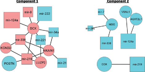
Of primary interest are the biological relations between the genes and miRNAs. Figure 11 displays a network of possible gene–miRNA interactions for each of the first two joint components, constructed from genes and miRNAs with large absolute loadings. A gene–miRNA pair is linked if the miRNA is predicted to regulate the expression of the gene, based on its DNA sequence. In particular, we use the mirWalk target prediction module [Dweep et al. (2011)] and include those pairs that are given in two or more of the miRNA target databases miRanda, Pictar, RNA22 and TargetScan. We caution that current methods to predict miRNA targets are inexact, and linked gene–miRNA pairs only indicate potential causal relations. Nevertheless, each joint component includes several predicted gene–miRNA interactions.

We further examine the individual genes and miRNAs that contribute the most to the first two joint components. The POSTN gene, which has the largest loading among genes in the first joint component, encodes the protein Periostine. Over-expression of Periostine is frequently reported in cancerous tumor cells and is suspected to facilitate cell motility (the ability of a cancer cell to migrate quickly and spontaneously) [Gillan et al. (2002)]. In GBM, the downregulation of POSTN expression by mir-219 has recently been linked to differences in survival and time to disease progression [Zinn et al. (2011)]. Interestingly, the miRNA mir-124a has the largest loading in both components, and a recent study suggests that this miRNA may also play an important role in GBM cell motility [Fowler et al. (2011)].

6 Summary and discussion

TCGA and similar projects are providing researchers with access to an increasing number of data sets that consist of multiple high-dimensional data types. However, there are relatively few general statistical methods for the analysis of such integrated data sets, and the unique features of JIVE provide a powerful new approach. JIVE finds both the coordinated activities of multiple data types, as well as those features unique to a particular data type. We demonstrate how accounting for joint structure can lead to better estimation of individual structure and vice versa. Our application of JIVE to gene and miRNA data on GBM tumor samples has provided better characterization of tumor types and better understanding of the biological interactions between the given data types.

JIVE does not require that the data are ordered, as in functional data analysis. Regularization techniques such as smoothing may improve the method for functional data. As pointed out by an Associate Editor, JIVE estimates for joint and individual structures are not robust to outliers. Exploratory methods such as PCA suffer similarly, and robust versions of PCA have recently been developed [see, e.g., Candes et al. (2009)]. A robust version of JIVE is an interesting potential extension. Further, any missing values must be imputed prior to computing JIVE estimates. An approach that explicitly accounts for missing values in the estimation of joint and individual structures is another potential extension.

The statistical properties of the algorithm also deserve further attention. In particular, measures of confidence (e.g., for variation explained by joint and individual structures) would be useful. Standard resampling techniques such as bootstrapping may help in this regard. However, factors such as the discrete nature of the ranks must be considered carefully.

While this paper focuses on vertically integrated biomedical data, the JIVE model and algorithm are very general and may be useful in other contexts. A similar approach can be applied to horizontally integrated data, in which disparate sets of samples (e.g., sick and healthy patients) are available on the same data type. In finance, JIVE has the potential to improve on current models that explain variation across and within disparate markets [see Bekaert, Hodrick and Zhang (2009)]. These applications are currently under study.

References

- Adourian et al. (2008) {barticle}[author] \bauthor\bsnmAdourian, \bfnmA.\binitsA., \bauthor\bsnmJennings, \bfnmE.\binitsE., \bauthor\bsnmBalasubramanian, \bfnmR.\binitsR., \bauthor\bsnmHines, \bfnmW.\binitsW., \bauthor\bsnmDamian, \bfnmD.\binitsD., \bauthor\bsnmPlasterer, \bfnmT.\binitsT., \bauthor\bsnmClish, \bfnmC.\binitsC., \bauthor\bsnmStroobant, \bfnmP.\binitsP., \bauthor\bsnmMcBurney, \bfnmR.\binitsR., \bauthor\bsnmVerheij, \bfnmE.\binitsE., \bauthor\bsnmBobeldijk, \bfnmI.\binitsI., \bauthor\bsnmGreef, \bfnmJ.\binitsJ., \bauthor\bsnmLindberg, \bfnmJ.\binitsJ., \bauthor\bsnmKenne, \bfnmK.\binitsK., \bauthor\bsnmAndersson, \bfnmU.\binitsU., \bauthor\bsnmHellmold, \bfnmH.\binitsH., \bauthor\bsnmNilsson, \bfnmK.\binitsK., \bauthor\bsnmSalterd, \bfnmH.\binitsH. and \bauthor\bsnmSchuppe-Koistinenc, \bfnmI.\binitsI. (\byear2008). \btitleCorrelation network analysis for data integration and biomarker selection. \bjournalMolecular BioSystems \bvolume4 \bpages249–259. \bptokimsref \endbibitem
- Bekaert, Hodrick and Zhang (2009) {barticle}[author] \bauthor\bsnmBekaert, \bfnmG.\binitsG., \bauthor\bsnmHodrick, \bfnmR.\binitsR. and \bauthor\bsnmZhang, \bfnmX.\binitsX. (\byear2009). \btitleInternational stock return comovements. \bjournalJ. Finance \bvolume64 \bpages2591–2626. \bptokimsref \endbibitem
- Bredel et al. (2009) {barticle}[pbm] \bauthor\bsnmBredel, \bfnmMarkus\binitsM., \bauthor\bsnmScholtens, \bfnmDenise M.\binitsD. M., \bauthor\bsnmHarsh, \bfnmGriffith R.\binitsG. R., \bauthor\bsnmBredel, \bfnmClaudia\binitsC., \bauthor\bsnmChandler, \bfnmJames P.\binitsJ. P., \bauthor\bsnmRenfrow, \bfnmJaclyn J.\binitsJ. J., \bauthor\bsnmYadav, \bfnmAjay K.\binitsA. K., \bauthor\bsnmVogel, \bfnmHannes\binitsH., \bauthor\bsnmScheck, \bfnmAdrienne C.\binitsA. C., \bauthor\bsnmTibshirani, \bfnmRobert\binitsR. and \bauthor\bsnmSikic, \bfnmBranimir I.\binitsB. I. (\byear2009). \btitleA network model of a cooperative genetic landscape in brain tumors. \bjournalJAMA \bvolume302 \bpages261–275. \biddoi=10.1001/jama.2009.997, issn=1538-3598, pii=302/3/261, pmid=19602686 \bptokimsref \endbibitem
- Cabanski et al. (2010) {barticle}[pbm] \bauthor\bsnmCabanski, \bfnmChristopher R.\binitsC. R., \bauthor\bsnmQi, \bfnmYuan\binitsY., \bauthor\bsnmYin, \bfnmXiaoying\binitsX., \bauthor\bsnmBair, \bfnmEric\binitsE., \bauthor\bsnmHayward, \bfnmMichele C.\binitsM. C., \bauthor\bsnmFan, \bfnmCheng\binitsC., \bauthor\bsnmLi, \bfnmJianying\binitsJ., \bauthor\bsnmWilkerson, \bfnmMatthew D.\binitsM. D., \bauthor\bsnmMarron, \bfnmJ. S.\binitsJ. S., \bauthor\bsnmPerou, \bfnmCharles M.\binitsC. M. and \bauthor\bsnmHayes, \bfnmD. Neil\binitsD. N. (\byear2010). \btitleSWISS MADE: Standardized within class sum of squares to evaluate methodologies and dataset elements. \bjournalPLoS ONE \bvolume5 \bpagese9905. \biddoi=10.1371/journal.pone.0009905, issn=1932-6203, pmcid=2845619, pmid=20360852 \bptokimsref \endbibitem
- Cancer Genome Atlas Research Network (2008) {bmisc}[auto] \borganizationCancer Genome Atlas Research Network (\byear2008). \bhowpublishedComprehensive genomic characterization defines human glioblastoma genes and core pathways. Nature 455 1061–1068. \biddoi=10.1038/nature07385, issn=1476-4687, mid=NIHMS68048, pii=nature07385, pmcid=2671642, pmid=18772890 \bptokimsref \endbibitem
- Candes et al. (2009) {bmisc}[author] \bauthor\bsnmCandes, \bfnmE.\binitsE., \bauthor\bsnmLi, \bfnmX.\binitsX., \bauthor\bsnmMa, \bfnmY.\binitsY. and \bauthor\bsnmWright, \bfnmJ.\binitsJ. (\byear2009). \bhowpublishedRobust principal component analysis? Available at arXiv:\arxivurl0912.3599. \bptokimsref \endbibitem
- Di et al. (2009) {barticle}[mr] \bauthor\bsnmDi, \bfnmChong-Zhi\binitsC.-Z., \bauthor\bsnmCrainiceanu, \bfnmCiprian M.\binitsC. M., \bauthor\bsnmCaffo, \bfnmBrian S.\binitsB. S. and \bauthor\bsnmPunjabi, \bfnmNaresh M.\binitsN. M. (\byear2009). \btitleMultilevel functional principal component analysis. \bjournalAnn. Appl. Stat. \bvolume3 \bpages458–488. \biddoi=10.1214/08-AOAS206, issn=1932-6157, mr=2668715 \bptokimsref \endbibitem
- Dweep et al. (2011) {barticle}[pbm] \bauthor\bsnmDweep, \bfnmHarsh\binitsH., \bauthor\bsnmSticht, \bfnmCarsten\binitsC., \bauthor\bsnmPandey, \bfnmPriyanka\binitsP. and \bauthor\bsnmGretz, \bfnmNorbert\binitsN. (\byear2011). \btitlemiRWalk-database: Prediction of possible miRNA binding sites by “walking” the genes of three genomes. \bjournalJ. Biomed. Inform. \bvolume44 \bpages839–847. \biddoi=10.1016/j.jbi.2011.05.002, issn=1532-0480, pii=S1532-0464(11)00078-5, pmid=21605702 \bptokimsref \endbibitem
- Fowler et al. (2011) {barticle}[author] \bauthor\bsnmFowler, \bfnmA.\binitsA., \bauthor\bsnmThompson, \bfnmD.\binitsD., \bauthor\bsnmGiles, \bfnmK.\binitsK., \bauthor\bsnmMaleki, \bfnmS.\binitsS., \bauthor\bsnmMreich, \bfnmE.\binitsE., \bauthor\bsnmWheeler, \bfnmH.\binitsH., \bauthor\bsnmLeedman, \bfnmP.\binitsP., \bauthor\bsnmBiggs, \bfnmM.\binitsM., \bauthor\bsnmCook, \bfnmR.\binitsR., \bauthor\bsnmLittle, \bfnmN.\binitsN., \bauthor\bsnmRobinson, \bfnmB.\binitsB. and \bauthor\bsnmMcDonald, \bfnmK.\binitsK. (\byear2011). \btitlemiR-124a is frequently down-regulated in glioblastoma and is involved in migration and invasion. \bjournalEuropean Journal of Cancer \bvolume47 \bpages953–963. \bptokimsref \endbibitem
- Galberin and Cochrane (2011) {barticle}[author] \bauthor\bsnmGalberin, \bfnmM.\binitsM. and \bauthor\bsnmCochrane, \bfnmG.\binitsG. (\byear2011). \btitleThe 2011 nucleic acids research database issue and the online molecular biology database collection. \bjournalNucleic Acids Res. \bvolume39 \bpagesD1–D6. \bptokimsref \endbibitem
- Gilad, Rifkin and Pritchard (2008) {barticle}[pbm] \bauthor\bsnmGilad, \bfnmYoav\binitsY., \bauthor\bsnmRifkin, \bfnmScott A.\binitsS. A. and \bauthor\bsnmPritchard, \bfnmJonathan K.\binitsJ. K. (\byear2008). \btitleRevealing the architecture of gene regulation: The promise of eQTL studies. \bjournalTrends Genet. \bvolume24 \bpages408–415. \biddoi=10.1016/j.tig.2008.06.001, issn=0168-9525, mid=NIHMS71884, pii=S0168-9525(08)00177-7, pmcid=2583071, pmid=18597885 \bptokimsref \endbibitem
- Gillan et al. (2002) {barticle}[author] \bauthor\bsnmGillan, \bfnmL.\binitsL., \bauthor\bsnmMatei, \bfnmD.\binitsD., \bauthor\bsnmFishman, \bfnmD.\binitsD., \bauthor\bsnmGerbin, \bfnmC.\binitsC., \bauthor\bsnmKarlan, \bfnmB.\binitsB. and \bauthor\bsnmChang, \bfnmD.\binitsD. (\byear2002). \btitlePeriostin secreted by epithelial ovarian carcinoma is a ligand for alpha(V)beta(3) and alpha(V)beta(5) integrins and promotes cell motility. \bjournalCancer Research \bvolume62 \bpages5358–5364. \bptokimsref \endbibitem
- Hotelling (1936) {barticle}[author] \bauthor\bsnmHotelling, \bfnmH.\binitsH. (\byear1936). \btitleRelations between two sets of variates. \bjournalBiometrika \bvolume28 \bpages321–377. \bptokimsref \endbibitem
- Lê Cao et al. (2008) {barticle}[mr] \bauthor\bsnmLê Cao, \bfnmKim-Anh\binitsK.-A., \bauthor\bsnmRossouw, \bfnmDebra\binitsD., \bauthor\bsnmRobert-Granié, \bfnmChristèle\binitsC. and \bauthor\bsnmBesse, \bfnmPhilippe\binitsP. (\byear2008). \btitleA sparse PLS for variable selection when integrating omics data. \bjournalStat. Appl. Genet. Mol. Biol. \bvolume7 \bpagesArt. 35, 31. \biddoi=10.2202/1544-6115.1390, issn=1544-6115, mr=2457048 \bptokimsref \endbibitem
- Lee et al. (2010) {barticle}[mr] \bauthor\bsnmLee, \bfnmMihee\binitsM., \bauthor\bsnmShen, \bfnmHaipeng\binitsH., \bauthor\bsnmHuang, \bfnmJianhua Z.\binitsJ. Z. and \bauthor\bsnmMarron, \bfnmJ. S.\binitsJ. S. (\byear2010). \btitleBiclustering via sparse singular value decomposition. \bjournalBiometrics \bvolume66 \bpages1087–1095. \biddoi=10.1111/j.1541-0420.2010.01392.x, issn=0006-341X, mr=2758496 \bptokimsref \endbibitem
- Lock et al. (2012) {bmisc}[author] \bauthor\bsnmLock, \bfnmE.\binitsE., \bauthor\bsnmHoadley, \bfnmK.\binitsK., \bauthor\bsnmMarron, \bfnmJ.\binitsJ. and \bauthor\bsnmNobel, \bfnmA.\binitsA. (\byear2012). \bhowpublishedSupplement to “Joint and individual variation explained (JIVE) for integrated analysis of multiple data types”. DOI:\doiurl10.1214/12-AOAS597SUPP. \bptokimsref \endbibitem
- Parkhomenko, Tritchler and Beyene (2009) {barticle}[mr] \bauthor\bsnmParkhomenko, \bfnmElena\binitsE., \bauthor\bsnmTritchler, \bfnmDavid\binitsD. and \bauthor\bsnmBeyene, \bfnmJoseph\binitsJ. (\byear2009). \btitleSparse canonical correlation analysis with application to genomic data integration. \bjournalStat. Appl. Genet. Mol. Biol. \bvolume8 \bpagesArt. 1, 36. \biddoi=10.2202/1544-6115.1406, issn=1544-6115, mr=2471148 \bptokimsref \endbibitem
- Parkinson et al. (2009) {barticle}[author] \bauthor\bsnmParkinson, \bfnmH.\binitsH., \bauthor\bsnmKapushesky, \bfnmM.\binitsM., \bauthor\bsnmKolesnikov, \bfnmN.\binitsN., \bauthor\bsnmRustici, \bfnmG.\binitsG., \bauthor\bsnmShojatalab, \bfnmM.\binitsM., \bauthor\bsnmAbeygunawardena, \bfnmN.\binitsN., \bauthor\bsnmBerube, \bfnmH.\binitsH., \bauthor\bsnmDylag, \bfnmM.\binitsM., \bauthor\bsnmEmam, \bfnmI.\binitsI., \bauthor\bsnmFarne, \bfnmA.\binitsA., \bauthor\bsnmHolloway, \bfnmE.\binitsE., \bauthor\bsnmLukk, \bfnmM.\binitsM., \bauthor\bsnmMalone, \bfnmJ.\binitsJ., \bauthor\bsnmMani, \bfnmR.\binitsR., \bauthor\bsnmPilicheva, \bfnmE.\binitsE., \bauthor\bsnmRayner, \bfnmT.\binitsT., \bauthor\bsnmRezwan, \bfnmF.\binitsF., \bauthor\bsnmSharma, \bfnmA.\binitsA., \bauthor\bsnmWilliams, \bfnmE.\binitsE., \bauthor\bsnmBradley, \bfnmX.\binitsX., \bauthor\bsnmAdamusiak, \bfnmT.\binitsT., \bauthor\bsnmBrandizi, \bfnmM.\binitsM., \bauthor\bsnmBurdett, \bfnmT.\binitsT., \bauthor\bsnmCoulson, \bfnmR.\binitsR., \bauthor\bsnmKrestyaninova, \bfnmM.\binitsM., \bauthor\bsnmKurnosov, \bfnmP.\binitsP., \bauthor\bsnmMaguire, \bfnmE.\binitsE., \bauthor\bsnmNeogi, \bfnmS.\binitsS., \bauthor\bsnmRocca-Serra, \bfnmP.\binitsP., \bauthor\bsnmSansone, \bfnmS.\binitsS., \bauthor\bsnmSklyar, \bfnmN.\binitsN., \bauthor\bsnmZhao, \bfnmM.\binitsM., \bauthor\bsnmSarkans, \bfnmU.\binitsU. and \bauthor\bsnmBrazma, \bfnmA.\binitsA. (\byear2009). \btitleArrayExpress update—from an archive of functional genomics experiments to the atlas of gene expression. \bjournalNucleic Acids Res. \bvolume37 \bpages868–872. \bptokimsref \endbibitem
- Peter (2010) {barticle}[pbm] \bauthor\bsnmPeter, \bfnmM. E.\binitsM. E. (\byear2010). \btitleTargeting of mRNAs by multiple miRNAs: The next step. \bjournalOncogene \bvolume29 \bpages2161–2164. \biddoi=10.1038/onc.2010.59, issn=1476-5594, pii=onc201059, pmid=20190803 \bptokimsref \endbibitem
- Rhead et al. (2010) {barticle}[author] \bauthor\bsnmRhead, \bfnmB.\binitsB., \bauthor\bsnmKarolchik, \bfnmD.\binitsD., \bauthor\bsnmKuhn, \bfnmR.\binitsR., \bauthor\bsnmHinrichs, \bfnmA.\binitsA., \bauthor\bsnmZweig, \bfnmA.\binitsA., \bauthor\bsnmFujita, \bfnmP.\binitsP., \bauthor\bsnmDiekhans, \bfnmM.\binitsM., \bauthor\bsnmSmith, \bfnmK.\binitsK., \bauthor\bsnmRosenbloom, \bfnmK.\binitsK., \bauthor\bsnmRaney, \bfnmB.\binitsB., \bauthor\bsnmPohl, \bfnmA.\binitsA., \bauthor\bsnmPheasant, \bfnmM.\binitsM., \bauthor\bsnmMeyer, \bfnmL.\binitsL., \bauthor\bsnmLearned, \bfnmK.\binitsK., \bauthor\bsnmHsu, \bfnmF.\binitsF., \bauthor\bsnmHillman-Jackson, \bfnmJ.\binitsJ., \bauthor\bsnmHarte, \bfnmR.\binitsR., \bauthor\bsnmGiardine, \bfnmB.\binitsB., \bauthor\bsnmDreszer, \bfnmT.\binitsT., \bauthor\bsnmClawson, \bfnmH.\binitsH., \bauthor\bsnmBarber, \bfnmG.\binitsG., \bauthor\bsnmHaussler, \bfnmD.\binitsD. and \bauthor\bsnmKent, \bfnmW.\binitsW. (\byear2010). \btitleThe UCSC genome browser database: Update 2010. \bjournalNucleic Acids Res. \bvolume38 \bpages613–619. \bptokimsref \endbibitem
- Schwarz (1978) {barticle}[mr] \bauthor\bsnmSchwarz, \bfnmGideon\binitsG. (\byear1978). \btitleEstimating the dimension of a model. \bjournalAnn. Statist. \bvolume6 \bpages461–464. \bidissn=0090-5364, mr=0468014 \bptokimsref \endbibitem
- Shen and Huang (2008) {barticle}[mr] \bauthor\bsnmShen, \bfnmHaipeng\binitsH. and \bauthor\bsnmHuang, \bfnmJianhua Z.\binitsJ. Z. (\byear2008). \btitleSparse principal component analysis via regularized low rank matrix approximation. \bjournalJ. Multivariate Anal. \bvolume99 \bpages1015–1034. \biddoi=10.1016/j.jmva.2007.06.007, issn=0047-259X, mr=2419336 \bptokimsref \endbibitem
- Shen, Olshen and Ladanyi (2009) {barticle}[pbm] \bauthor\bsnmShen, \bfnmRonglai\binitsR., \bauthor\bsnmOlshen, \bfnmAdam B.\binitsA. B. and \bauthor\bsnmLadanyi, \bfnmMarc\binitsM. (\byear2009). \btitleIntegrative clustering of multiple genomic data types using a joint latent variable model with application to breast and lung cancer subtype analysis. \bjournalBioinformatics \bvolume25 \bpages2906–2912. \biddoi=10.1093/bioinformatics/btp543, issn=1367-4811, pii=btp543, pmcid=2800366, pmid=19759197 \bptokimsref \endbibitem
- Sporns, Tononi and Kötter (2005) {barticle}[pbm] \bauthor\bsnmSporns, \bfnmOlaf\binitsO., \bauthor\bsnmTononi, \bfnmGiulio\binitsG. and \bauthor\bsnmKötter, \bfnmRolf\binitsR. (\byear2005). \btitleThe human connectome: A structural description of the human brain. \bjournalPLoS Comput. Biol. \bvolume1 \bpagese42. \biddoi=10.1371/journal.pcbi.0010042, issn=1553-7358, pmcid=1239902, pmid=16201007 \bptokimsref \endbibitem
- Tibshirani (1996) {barticle}[mr] \bauthor\bsnmTibshirani, \bfnmRobert\binitsR. (\byear1996). \btitleRegression shrinkage and selection via the lasso. \bjournalJ. Roy. Statist. Soc. Ser. B \bvolume58 \bpages267–288. \bidissn=0035-9246, mr=1379242 \bptokimsref \endbibitem
- Trygg and Wold (2003) {barticle}[author] \bauthor\bsnmTrygg, \bfnmJ.\binitsJ. and \bauthor\bsnmWold, \bfnmS.\binitsS. (\byear2003). \btitleO2-PLS, a two-block (X-Y) latent variable regression (LVR) method with an integral OSC filter. \bjournalJournal of Chemometrics \bvolume17 \bpages53–64. \bptokimsref \endbibitem
- Verhaak et al. (2010) {barticle}[pbm] \bauthor\bsnmVerhaak, \bfnmRoel G. W.\binitsR. G. W., \bauthor\bsnmHoadley, \bfnmKatherine A.\binitsK. A., \bauthor\bsnmPurdom, \bfnmElizabeth\binitsE., \bauthor\bsnmWang, \bfnmVictoria\binitsV., \bauthor\bsnmQi, \bfnmYuan\binitsY., \bauthor\bsnmWilkerson, \bfnmMatthew D.\binitsM. D., \bauthor\bsnmMiller, \bfnmC. Ryan\binitsC. R., \bauthor\bsnmDing, \bfnmLi\binitsL., \bauthor\bsnmGolub, \bfnmTodd\binitsT., \bauthor\bsnmMesirov, \bfnmJill P.\binitsJ. P., \bauthor\bsnmAlexe, \bfnmGabriele\binitsG., \bauthor\bsnmLawrence, \bfnmMichael\binitsM., \bauthor\bsnmO’Kelly, \bfnmMichael\binitsM., \bauthor\bsnmTamayo, \bfnmPablo\binitsP., \bauthor\bsnmWeir, \bfnmBarbara A.\binitsB. A., \bauthor\bsnmGabriel, \bfnmStacey\binitsS., \bauthor\bsnmWinckler, \bfnmWendy\binitsW., \bauthor\bsnmGupta, \bfnmSupriya\binitsS., \bauthor\bsnmJakkula, \bfnmLakshmi\binitsL., \bauthor\bsnmFeiler, \bfnmHeidi S.\binitsH. S., \bauthor\bsnmHodgson, \bfnmJ. Graeme\binitsJ. G., \bauthor\bsnmJames, \bfnmC. David\binitsC. D., \bauthor\bsnmSarkaria, \bfnmJann N.\binitsJ. N., \bauthor\bsnmBrennan, \bfnmCameron\binitsC., \bauthor\bsnmKahn, \bfnmAri\binitsA., \bauthor\bsnmSpellman, \bfnmPaul T.\binitsP. T., \bauthor\bsnmWilson, \bfnmRichard K.\binitsR. K., \bauthor\bsnmSpeed, \bfnmTerence P.\binitsT. P., \bauthor\bsnmGray, \bfnmJoe W.\binitsJ. W., \bauthor\bsnmMeyerson, \bfnmMatthew\binitsM., \bauthor\bsnmGetz, \bfnmGad\binitsG., \bauthor\bsnmPerou, \bfnmCharles M.\binitsC. M., \bauthor\bsnmHayes, \bfnmD. Neil\binitsD. N. and \bauthor\bsnmCancer Genome Atlas Research Network (\byear2010). \btitleIntegrated genomic analysis identifies clinically relevant subtypes of glioblastoma characterized by abnormalities in PDGFRA, IDH1, EGFR, and NF1. \bjournalCancer Cell \bvolume17 \bpages98–110. \biddoi=10.1016/j.ccr.2009.12.020, issn=1878-3686, mid=NIHMS166306, pii=S1535-6108(09)00432-2, pmcid=2818769, pmid=20129251 \bptokimsref \endbibitem
- Westerhuis, Kourti and MacGregor (1998) {barticle}[author] \bauthor\bsnmWesterhuis, \bfnmJ.\binitsJ., \bauthor\bsnmKourti, \bfnmT.\binitsT. and \bauthor\bsnmMacGregor, \bfnmJ.\binitsJ. (\byear1998). \btitleAnalysis of multiblock and hierarchical PCA and PLS models. \bjournalJournal of Chemometrics \bvolume12 \bpages301–321. \bptokimsref \endbibitem
- Witten and Tibshirani (2009) {barticle}[mr] \bauthor\bsnmWitten, \bfnmDaniela M.\binitsD. M. and \bauthor\bsnmTibshirani, \bfnmRobert J.\binitsR. J. (\byear2009). \btitleExtensions of sparse canonical correlation analysis with applications to genomic data. \bjournalStat. Appl. Genet. Mol. Biol. \bvolume8 \bpagesArt. 28, 29. \biddoi=10.2202/1544-6115.1470, issn=1544-6115, mr=2533636 \bptokimsref \endbibitem
- Wold (1985) {bincollection}[author] \bauthor\bsnmWold, \bfnmH.\binitsH. (\byear1985). \btitlePartial Least Squares. In \bbooktitleEncyclopedia of Statistical Sciences (Vol. 6) (\beditor\bfnmS.\binitsS. \bsnmKotz and \beditor\bfnmN.\binitsN. \bsnmJohnson, eds.) \bpages581–591. \bpublisherWiley, \blocationNew York. \bptokimsref \endbibitem
- Wold, Kettaneh and Tjessem (1996) {barticle}[author] \bauthor\bsnmWold, \bfnmS.\binitsS., \bauthor\bsnmKettaneh, \bfnmN.\binitsN. and \bauthor\bsnmTjessem, \bfnmK.\binitsK. (\byear1996). \btitleHierarchical multiblock PLS and PC models for easier model interpretation and as an alternative to variable selection. \bjournalJournal of Chemometrics \bvolume10 \bpages463–482. \bptokimsref \endbibitem
- Zinn et al. (2011) {barticle}[author] \bauthor\bsnmZinn, \bfnmP.\binitsP., \bauthor\bsnmMajadan, \bfnmB.\binitsB., \bauthor\bsnmSathyan, \bfnmP.\binitsP., \bauthor\bsnmSingh, \bfnmK.\binitsK., \bauthor\bsnmMajumder, \bfnmS.\binitsS., \bauthor\bsnmJolesz, \bfnmF.\binitsF. and \bauthor\bsnmColen, \bfnmR.\binitsR. (\byear2011). \btitleRadiogenomic mapping of edema/cellular invasion MRI-phenotypes in glioblastoma multiforme. \bjournalPLoS ONE \bvolume6 \bpagese25451. \bptokimsref \endbibitem