Closed form solution for the self-resonances in a short Josephson junction

Abstract

We present a closed form solution for the self-resonances in a short Josephson tunnel junction. This solution is alternative to the well known textbook result [1, 2] based on a series expansion. Results are derived for the up-to-date case of a $0-\pi$ junction.

When a constant voltage $V$ is present across the electrodes of a Josephson junction, the current flowing into the junction oscillates at a frequency $\omega=2\pi V/\Phi_{0}$, where $\Phi_{0}=2.07\times 10^{-15}$ Weber is the flux quantum. On the other hand, if the major size of the junction $L$ is shorter than the Josephson penetration depth $\lambda_{j}$ (short junction limit), the junction can be viewed as a cavity of length $L$. In the presence of a uniform magnetic field and at an applied junction voltage $V_{n}=\Phi_{0}\omega_{n}/2\pi$, the oscillation frequency of the Josephson current matches the n-th harmonic of the junction cavity mode resulting in the excitation of some of the modes at the frequencies $\omega_{n}/2\pi=n\bar{c}/2L$ (n = 1,2,3…), where $\bar{c}$ is the light velocity of the waves in the resonator. In this case typical current ’steps’, known as ’Fiske steps’ [3], appear in the $I-V$ characteristic of the junction [1].

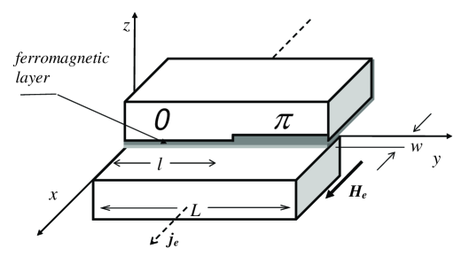
Figure 1: Schematic of the superconductor-insulator-ferromagnetic metal-superconductor $0-\pi$ Josephson tunnel junction, along with the coordinate system used in this work

Kulik [2] showed how to calculate, in agreement with the experiments [3], the dependence of the amplitude of these steps as a function of an applied magnetic field in the short junction limit. In the Kulik’s solution, the Josephson phase difference is expressed in the form of a Fourier series, each term representing one of the resonances at the voltages $V_{n}$. Fiske steps are observed also in long junctions ($L>\lambda_{j}$), when a magnetic field is externally applied. In this case however the junction behaves more like a transmission line than a resonator and relevant to the underlaying mechanism is the presence of so called fluxons, particle-like current-field structures periodically driven inside the junction [4].

In this letter we present and discuss an alternative equivalent approach we have developed for calculating the Fiske resonances in a short Josephson junction. The method is based on the development of a closed form solution to the linearized sine-Gordon equation. Compared to the standard result this method may present some advantages, in particular if one is interested to a description of the phase dynamics given in closed form. We apply the method to the relevant case of a $0-\pi$ Josephson junction, i.e. a junction which has a coupling, changing between $0$ and $\pi$ along the junction length, which implies an anomalous current-phase relation in the $\pi$-region (see equation(3)). This physical situation can be realized, for instance, in superconductor-insulator-ferromagnetic metal-superconductor tunnel junctions, i.e. junctions in which a ferromagnetic layer with step-like thickness is inserted, in addition to an insulating layer [5, 6] (see figure 1).

The effect of the presence of few, or many, adjacent $0-\pi$ phase shifts on the self resonant modes of a Josephson junction has been considered in the context of YBCO grain boundary Josephson junctions [7]. In that reference, in order to calculate the contribution of the self-resonances to the current-voltage characteristics, an extension of the Kulik expansion was developed. The results have been successfully used to fit data on Fiske steps in $0-\pi$ Josephson tunnel junctions [8]. Also recently, a careful analysis of Fiske modes, based on the Kulik theory, has been carried out in superconductor-insulator-ferromagnetic metal-superconductor to extract information on the junction quality factor and the relevant damping mechanisms [9].

Let us consider a $0-\pi$ junction with two adjacent regions $[0,\l]$ and $[\l,L]$, characterized by two different maximum Josephson current densities, $j_{1}$ and $j_{2}$ ($j_{1}>0$ and $j_{2}>0$) and a $\pi$ phase shift in region $[\l,L]$ (See figure 1). The supercurrent density can be written as

$$J(y)=J_{c}(y)\sin\ \left[\varphi+\pi\theta(y-l)\right]=\left\{\begin{array}[]{rl}j_{1}\sin(\varphi)&\textrm{if $0<y<\l$}\\ j_{2}\sin(\varphi+\pi)&\textrm{if $\l<y<L$}\end{array}\right.$$ (3)

Assuming a one-dimensional system ($w<<L$), the equation for the phase difference $\varphi(y,t)$ is expressed by

$$\langle\lambda_{j}\rangle^{2}\frac{\partial^{2}\varphi}{\partial y^{2}}-\frac{1}{\langle\omega_{p}\rangle^{2}}\frac{\partial^{2}\varphi}{\partial t^{2}}-\frac{1}{{{RC\langle\omega_{p}\rangle}^{2}}}\frac{\partial\varphi}{\partial t}=\frac{J_{c}(y)}{\langle J_{c}\rangle}\sin\ \left[\varphi+\pi\theta(y-l)\right]-\frac{j_{e}}{\langle J_{c}\rangle}$$ (4)

where we have introduced the specific normal resistance $R$ and capacitance $C$ of the junction. Function $\theta(y)$ is the Heaviside step function, $j_{e}/\langle{J_{c}}\rangle$ is the normalized external bias current density, and $\langle J_{c}\rangle=\left(j_{1}\l+j_{2}(L-\l)\right)/L$ is the average maximum Josephson current density. In Eq. 4 the average Josephson penetration depth is given by $\langle\lambda_{j}\rangle=\sqrt{\Phi_{0}/\left(2\pi\mu_{0}\langle J_{c}\rangle d_{eff}\right)}$ [7]where the effective depth is $d_{eff}\approx 2\lambda_{L}$ with $\lambda_{L}$ the London penetration length and we have introduced the average plasma frequency $\langle\omega_{p}\rangle=\sqrt{2\pi\langle J_{c}\rangle/\Phi_{0}C}$.

In the geometry of figure 1, the magnetic field within the junction is related to the derivative of $\varphi$ through the relationship

$$H(y)=-\frac{\Phi_{0}}{2\pi\mu_{0}d_{eff}}\left(\frac{d\varphi}{dy}\right)$$ (5)

The boundary conditions appropriate to equation (4), and to the considered geometry are

$$\left.\frac{\partial\varphi}{\partial y}\right|_{0}=\left.\frac{\partial\varphi}{\partial y}\right|_{L}=-\frac{2\pi\mu_{0}d_{eff}H_{e}}{\Phi_{0}}$$ (6)

Further important conditions are given by the continuity of $\varphi$ and of its derivative at the point $y=\l$. The last condition expresses the continuity of the magnetic field. From now on, all lengths and time variables will be normalized to $\langle\lambda_{j}\rangle$ and to the inverse average plasma frequency $\langle\omega_{p}\rangle$, respectively, so that equations (4) and (6) become respectively

$$\varphi_{yy}-\varphi_{tt}-\alpha\varphi_{t}=\frac{J_{c}(y)}{\langle J_{c}\rangle}\sin\left[\varphi+\pi\theta(y-l)\right]-\frac{j_{e}}{\langle J_{c}\rangle},$$ (7)

$$\varphi_{y}(0,t)=\varphi_{y}(L,t)=-h_{e},$$ (8)

where $\alpha=1/Q=1/\langle\omega_{p}\rangle RC$ is the dimensionless damping coefficient, $Q$ the damping quality factor and $h_{e}=H_{e}/\langle\lambda_{j}\rangle\langle J_{c}\rangle$ is the normalized external magnetic field.

Following the Kulik approximation, for solving equation (4) we write the phase $\varphi$ as a sum of two terms $\varphi(y,t)=\varphi_{0}(y,t)+\varphi_{1}(y,t)$ where the unperturbed term is $\varphi_{0}=\omega t-h_{e}y$, $\varphi_{1}\ll\varphi_{0}$ and $v=\Phi_{0}/2\pi d\varphi_{1}/dt$ is the perturbation to the steady voltage $V$. Here $\omega=\left(2\pi V/\Phi_{0}\right)/\langle\omega_{p}\rangle$ is the normalized Josephson frequency corresponding to the fixed voltage $V$ applied between the electrodes of the junction. We note that, to the zero-$th$ order, no magnetic field is associated with the $0-\pi$ discontinuity in the present approximation, as on the left and right of the point $y=l$ we have $d\varphi_{0}/dy=-h_{e}$, and the only magnetic field present is the external one. A time dependent magnetic field perturbation however appears to the 1st order, i.e. $\partial\varphi_{1}/\partial y$.

If we denote the perturbation $\varphi_{1}$ as $\varphi_{1}^{L}$, when considered in the interval $0\leq y\leq\l$, and $\varphi_{1}^{R}$, when considered in the interval $\l\leq y\leq L$, the linear equations providing $\varphi_{1}^{L}$ and $\varphi_{1}^{R}$ are respectively

$$\frac{\partial^{2}\varphi_{1}^{L}}{\partial y^{2}}-\frac{\partial^{2}\varphi_{1}^{L}}{\partial t^{2}}-\alpha\frac{\partial\varphi_{1}^{L}}{\partial t}=g_{1}\sin\left(\omega t-h_{e}y\right)$$ (9)

for $0\leq y\leq\l$, and

$$\frac{\partial^{2}\varphi_{1}^{R}}{\partial y^{2}}-\frac{\partial^{2}\varphi_{1}^{R}}{\partial t^{2}}-\alpha\frac{\partial\varphi_{1}^{R}}{\partial t}=g_{2}\sin\left(\omega t-h_{e}y\right)$$ (10)

for $\l\leq y\leq L$. In equations (9) and (10) we have defined $g_{1}=j_{1}/\langle J_{c}\rangle$, $g_{2}=-j_{2}/\langle J_{c}\rangle$. The boundary conditions appropriate to equations (9) and (10) are

$$\frac{\partial\varphi_{1}^{L}(0,t)}{\partial y}=\frac{\partial\varphi_{1}^{R}(L,t)}{\partial y}=0$$ (11)

$$\varphi_{1}^{L}(\l,t)=\varphi_{1}^{R}(\l,t)$$ (12)

$$\frac{\partial\varphi_{1}^{L}(\l,t)}{\partial y}=\frac{\partial\varphi_{1}^{R}(\l,t)}{\partial y}$$ (13)

Equation (11) is the requirement of perfect reflectivity of the edges of the junction and continuity of the phase and of its first derivative at the point $y=\l$ are determined by the equations (12) and (13), respectively.

After defining the two complex functions $u(y)$ and $v(y)$ through the factorization

$$\varphi_{1}^{L}=Re\left[u(y)\exp(-i\omega t)\right]$$ (14)

$$\varphi_{1}^{R}=Re\left[v(y)\exp(-i\omega t)\right]$$ (15)

and substituting (14) and (15) in (9) and (10), we find that $u$ and $v$ satisfy the two equations

$$\frac{d^{2}u}{dy^{2}}+\chi^{2}u=ig_{1}\exp(ih_{e}y)$$ (16)

for $0\leq y\leq\l$, and

$$\frac{d^{2}v}{dy^{2}}+\chi^{2}v=ig_{2}\exp(ih_{e}y)$$ (17)

for $\l\leq y\leq L$, where we have defined $\chi^{2}=\left(\omega^{2}+i\alpha\omega\right)$. The boundary conditions for the two complex functions $u(y)$ and $v(y)$ are

$$\frac{du(0)}{dy}=\frac{dv(L)}{dy}=0$$ (18)

$$u(\l)=v(\l)$$ (19)

$$\frac{du(\l)}{dy}=\frac{dv(\l)}{dy}$$ (20)

We can write now the general solution to equations (16) and (17) in the following form

$$u(y)=\alpha_{u}e^{-i\chi y}+\beta_{u}e^{+i\chi y}+u_{p}(y),0\leq y\leq\l$$ (21)

$$v(y)=\alpha_{v}e^{-i\chi(y)}+\beta_{v}e^{+i\chi(y)}+v_{p}(y),\l\leq y\leq L$$ (22)

where the basic task reduces to determine the four constants $\alpha_{u}$, $\beta_{u}$, $\alpha_{v}$ , $\beta_{v}$ from the boundary conditions (18)-(20). In equations (21) and (22) we have introduced the particular solutions $u_{p}(y)$ and $v_{p}(y)$ which, by following standard methods, can be promptly written as

$$u_{p}(y)=\frac{ig_{1}e^{ih_{e}y}}{\chi^{2}-h_{e}^{2}}$$ (23)

$$v_{p}(y)=\frac{ig_{2}e^{ih_{e}y}}{\chi^{2}-h_{e}^{2}}$$ (24)

By using the boundary conditions (18)-(20) we find the following relationship between the unknown coefficients $\alpha_{u}$, $\beta_{u}$, $\alpha_{v}$ and $\beta_{v}$

$$i\chi\left(\alpha_{u}-\beta_{u}\right)=\frac{g_{1}h_{e}}{\chi^{2}-h_{e}^{2}}$$ (25)

$$i\chi\left(\alpha_{v}e^{i\chi L}-\beta_{v}e^{-i\chi L}\right)=\frac{g_{2}h_{e}e^{ih_{e}L}}{\chi^{2}-h_{e}^{2}}$$

$$\left(\alpha_{u}-\alpha_{v}\right)e^{i\chi l}+\left(\beta_{u}-\beta_{v}\right)e^{-i\chi l}=\frac{(g_{2}-g_{1})h_{e}e^{ih_{e}l}}{\chi^{2}-h_{e}^{2}}$$

$$i\chi\left(\alpha_{u}-\alpha_{v}\right)e^{i\chi l}+i\chi\left(\beta_{u}-\beta_{v}\right)e^{-i\chi l}=\frac{(g_{1}-g_{2})h_{e}e^{ih_{e}l}}{\chi^{2}-h_{e}^{2}}$$

From equations (23)-(25) we obtain $\alpha_{u}$, $\beta_{u}$, $\alpha_{v}$, which can be written as

$$\alpha_{u}=\frac{1}{2\chi(\sin\chi L)(\chi^{2}-h_{e}^{2})}\times$$ (26)

$$\left[(g_{2}-g_{1})e^{ih_{e}l}S(L-l)+h_{e}(g_{1}e^{-i\chi L}-g_{2}e^{ih_{e}L})\right]$$

$$\beta_{u}=\frac{1}{2\chi(\sin\chi L)(\chi^{2}-h_{e}^{2})}\times$$ (27)

$$\left[(g_{2}-g_{1})e^{ih_{e}l}S(L-l)+h_{e}(g_{1}e^{i\chi L}-g_{2}e^{ih_{e}L})\right]$$

$$\alpha_{v}=\frac{1}{2\chi(\sin\chi L)(\chi^{2}-h_{e}^{2})}\times$$ (28)

$$\left[(g_{2}-g_{1})e^{i(h_{e}l-\chi l)}S(-l)+h_{e}(g_{1}e^{-i\chi L}-g_{2}e^{ih_{e}L})\right]$$

$$\beta_{v}=\frac{1}{2\chi(\sin\chi L)(\chi^{2}-h_{e}^{2})}\times$$ (29)

$$\left[(g_{2}-g_{1})e^{i(h_{e}l+\chi l)}S(-l)+h_{e}(g_{1}e^{-i\chi L}-g_{2}e^{ih_{e}L})\right]$$

where $S(z)=h_{e}\cos{(\chi z)}+i\chi\sin{(\chi z)}$.
Equations (14), (15), and (21), (22), with coefficients (26), (27), (28) and (29), determine in the present approximation of ’small $Q$’ and short junction [1], the dynamics of the phase $\varphi_{1}$ and the magnetic field inside the junction $\partial\varphi_{1}/\partial y$ for arbitrary $\omega$ and $h_{e}$ values.

Next, in order to extract a possible dc term in the current, we have to carry out time and space averages. That is to say, we have to calculate the quantity

$$J_{dc}(\omega,h_{e})=\frac{1}{L}\int_{0}^{L}\langle J_{c}(y)\sin\varphi(y)\rangle dy=$$ (30)

$$= \frac{1}{L}\int_{0}^{L}\langle J_{c}(y)\sin(\varphi_{0}(y)+\varphi_{1}(y,t)+\pi\theta(\l-L))\rangle dy=$$

$$= \frac{1}{L}\left[j_{1}\int_{0}^{\l}\langle\sin(\varphi_{0}+\varphi_{1}^{L})\rangle dy-j_{2}\int_{\l}^{L}\langle\sin(\varphi_{0}+\varphi_{1}^{R})\rangle dy\right]$$

Angle brackets indicate time average over the period $T=2\pi/\omega$, i.e. if $F(t)$ is an arbitrary function of the time, then $\langle F(t)\rangle=(1/T)\int_{0}^{T}F(t)dt=(1/2\pi)\int_{0}^{2\pi}F(\omega t)d(\omega t)$. Furthermore, since $\langle\sin(\varphi_{0}+\varphi_{1})\rangle\approx\langle\sin\varphi_{0}\rangle+\langle\varphi_{1}\cos\varphi_{0}\rangle$ and

$$\langle\sin\varphi_{0}\rangle=0$$

$$\langle\varphi_{1}^{L}\cos\varphi_{0}\rangle=\frac{1}{2}Re\left[ue^{-ih_{e}y}\right]$$

$$\langle\varphi_{1}^{R}\cos\varphi_{0}\rangle=\frac{1}{2}Re\left[ve^{-ih_{e}y}\right]$$

we obtain for the dc component of the current due to the self- resonances, the expression

$$\frac{J_{dc}(\omega,h_{e})}{\langle J_{c}\rangle}=\frac{1}{2L}Re\left[g_{1}\int_{0}^{\l}ue^{-ih_{e}y}dy+g_{2}\int_{\l}^{L}ve^{-ih_{e}y}dy\right]$$ (32)

Figure 2: Current density vs $\omega$ in zero external magnetic field in a $0-\pi$ Josephson junction; $\alpha=1;L=1;h_{e}=0;l=0.5;g_{1}=1;g_{2}=-1;$ self-resonances appear only at the odd positions $\omega=\pi,3\pi,5\pi$

.

Figure 3: Current density vs $\omega$ in the presence of an external magnetic field in a $0-\pi$ Josephson junction. The two curves refer to two different values of the magnetic field ($h_{e}=11$ and $h_{e}=10$, thin and thick line respectively); $\alpha=1;L=1;l=0.5;g_{1}=1;g_{2}=-1;$

The result can be expressed in term of the normalized flux $\phi$ applied to the junction, with the position $h_{e}L=2\pi\phi=2\pi\Phi/\Phi_{0}$, where $\Phi=\mu_{0}H_{e}d_{eff}(L$ and $d_{eff}$ and $L$ are expressed in the usual units in the last expression). The coefficients, equations (26), (28) and (29), diverge for $\sin{\chi L}=0$ in the limit of vanishing damping. This gives the resonance frequencies of the system $\omega_{n}=n\pi/L$ and, with very good approximation, the frequencies at which, in the presence of damping, the current equation (32) peaks. The amplitude dependence of the $n-th$ step on the magnetic field, of fundamental importance for a comparison with the experiments [7],[8], can be calculated by equation (32) by setting the value of $\omega$ at $\omega=\omega_{n}$. The same equation can be also used to probe the ’shape’ of the resonances as a function of the frequency and $Q$ damping factor. For the sake of illustration, in figures 2 and 3 we show two cases of current versus frequency obtained by using equation (32). The first graph refers to the case of zero external field. As can be seen, odd resonances persist in zero field, even though the amplitudes of those following the first are vanishingly small, a phenomenon typical of the $0-\pi$ junction [7]. The second one refers to a generic situation of presence of an external magnetic field and the two curves are calculated at two different values of the normalized field. The right hand side of each of the bell shaped peak has negative resistance and, for this reason, has no relevance for a comparison with the experiments, where usually a current bias set up is considered. We point out that, in principle, in the framework of the Kulik theory [7], to obtain the same accuracy in the determination of the current density as a function of frequency or magnetic field, one would have to sum up the contributions of the entire series representing the current. Finally it is worthwhile to stress that the result for a $0-0$ tunnel junction, with uniform maximum Josephson current density, can be easily recovered by the above method. In this case we have to discuss only the equation

$$\frac{d^{2}u_{0}}{dy^{2}}+\chi^{2}u_{0}=i\exp(ih_{e}y)$$ (33)

with $0\leq y\leq L$, $\varphi_{1}=Re[u_{0}(y)exp(-i\omega t)]$ and the boundary conditions $du_{0}(0)/dy=du_{0}(L)/dy=0$. The solution can be written in the following form

$$u_{0}(y)=\alpha_{0}e^{-i\chi y}+\beta_{0}e^{i\chi y}+\frac{ie^{ih_{e}y}}{\chi^{2}-h_{e}^{2}},$$ (34)

only two coefficients $\alpha_{0}$ e $\beta_{0}$ have to be determined. These coefficients are obtained from the two boundary conditions since, now, the continuity condition at $l=0$ is no longer required and they are given by the following simple expressions

$$\alpha_{0}=\frac{1}{2\chi(\sin\chi L)(\chi^{2}-h_{e}^{2})}\left(e^{-i\chi L}-e^{ih_{e}L}\right)$$ (35)

$$\beta_{0}=\frac{1}{2\chi(\sin\chi L)(\chi^{2}-h_{e}^{2})}\left(e^{i\chi L}-e^{ih_{e}L}\right)$$

It is easy to verify that these coefficients can be formally obtained by (26)-(29) by letting $l=0$ and taking $g_{1}=g_{2}=1$. In the same limit, we can also determine from the general result given by equation (32), the explicit expression of the frequency and field dependance of the current density, namely

$$J_{dc}(\omega,h_{e})=Re\left[\frac{ih_{e}^{2}}{\chi L(\sin\chi L)(\chi^{2}-h_{e}^{2})^{2}}\left(\cos\chi L-\cos h_{e}L\right)+\frac{i}{2(\chi^{2}-h_{e}^{2})}\right]$$ (36)

In conclusion, we have presented and discussed a closed form solution for the determination of the dynamics of the phase in a Josephson junction in the limit of short junction. Within this framework we have also derived an expression for the dc current density associated to the Fiske resonances in a $0-\pi$ Josephson tunnel junction. This approach can be relevant for improving the accuracy of data fitting in the determination of the damping mechanism in $0-\pi$ Josephson junctions or conventional Josephson tunnel junctions.

References

[1] A. Barone and G. Paternó, Physics and Applications of the Josephson Effect
(Wiley, NY 1982)
[2]I. Kulik, JEPT Lett.2, 84 (1965)
[3] M.D. Fiske, Rev. Mod. Phys. 36(1), 221 (1964)
[4]O. H. Olsen and M. R. Samuelsen, J. Appl. Phys.52, 6247
(1981); C. Nappi, M. P. Lisitskiy, G. Rotoli, R. Cristiano, A.
Barone, Phys. Rev. Lett., 93 187001 (2004)
[5]M. Weides, M. Kemmler, H. Kohlstedt, R. Waser, D.
Koelle, R. Kleiner, E. Goldobin, Phys. Rev. Lett, 97, 247001 (2006)
[6] M. Weides, U. Peralagu, H. Kohlstedt, J. Pfeiffer, M. Kemmler,
C. Guerlich, E. Goldobin, D. Koelle, and R. Kleiner, Supercond.
Sci. Technol.23, 095007 (2010).
[7] C. Nappi, E. Sarnelli, M. Adamo, M. A. Navacerrada, Phys. Rev. B, 74, 144504 (2006)
[8] J. Pfeiffer, M. Kemmler, D. Koelle, R. Kleiner, E. Goldobin, M. Weides,
A. K. Feofanov, J. Lisenfeld, A. V. Ustinov Phys. Rev. B,
77, 214506 (2008)
[9] G. Wild, C. Probst, A. Marx, and R. Gross, Eur. Phys. J. B78, 509 523 (2010)