Transforming fixed-length self-avoiding walks
into radial SLE_8/3

Abstract

We conjecture a relationship between the scaling limit of the fixed-length ensemble of self-avoiding walks in the upper half plane and radial SLE_8/3 in this half plane from $0$ to $i$. The relationship is that if we take a curve from the fixed-length scaling limit of the SAW, weight it by a suitable power of the distance to the endpoint of the curve and then apply the conformal map of the half plane that takes the endpoint to $i$, then we get the same probability measure on curves as radial SLE_8/3. In addition to a non-rigorous derivation of this conjecture, we support it with Monte Carlo simulations of the SAW. Using the conjectured relationship between the SAW and radial SLE_8/3, our simulations give estimates for both the interior and boundary scaling exponents. The values we obtain are within a few hundredths of a percent of the conjectured values.

1 Introduction

Consider the uniform probability measure on all self-avoiding walks (SAW) with $N$ steps on a two dimensional lattice with spacing $\delta$, e.g., $\delta{\mathbb{Z}}^{2}$. We restrict to SAW’s that start at the origin and lie in the upper half plane thereafter. Now take $\delta=N^{-\nu}$ and let $N\rightarrow\infty$. This should give a probability measure on simple curves in the half plane that start at the origin and end somewhere in the half plane. We refer to this scaling limit as the fixed-length scaling limit. Radial SLE_8/3 gives a probability measure on simple curves in the half plane that start at the origin and end at some prescribed point. So it is natural to look for some relation between the fixed-length scaling limit of the SAW and radial SLE_8/3.

The simplest relation would be the following. Take a curve from the fixed-length scaling limit of the half plane SAW and apply the conformal map of the half plane to itself that fixes the origin and maps the endpoint of the curve to $i$. This transformation gives a probability measure on curves from the origin to $i$, and so one might ask if the resulting measure is radial SLE_8/3. Oded Schramm proposed a Monte Carlo study of this possibility to the author [21]. Simulations of the SAW gave strong evidence that these two probability measure are not the same. In this paper we will argue that this process of conformally mapping the endpoint of the SAW to $i$ does in fact give radial SLE_8/3 if one weights the walk by $R^{p}$ where $R$ is the distance from the origin to the endpoint of the walk taken from the fixed-length scaling limit. The power $p$ is conjectured to be $(\rho-\gamma)/\nu=-61/48$.

In addition to our heuristic derivation of this conjecture, we also provide Monte Carlo simulations of the SAW to support it. The Monte Carlo simulations show excellent agreement with analytic calculations done with radial SLE_8/3. We can also estimate the interior and exterior scaling exponents from the simulations and find values that are within a few hundredths of a percent of the conjectured values.

One can also consider an ensemble of SAW’s in the half plane that start at the origin and have any length. The walks are then weighted by $\mu^{-N}$ where $N$ is the length of the walk and $\mu$ is the lattice constant for the SAW on the lattice being used. The total weight of these walks is infinite, but SLE partition functions predict the relative weights of the walks that end at different points in the upper half plane. Our simulations of the SAW also provide a partial test of this prediction. More precisely, we are able to test the angular dependence of the prediction. Once again excellent agreement is found.

In section 2 we quickly review several different scaling limits one can take for the SAW and their conjectured relationships with chordal and radial SLE_8/3. We also review several critical exponents for the SAW and review SLE partition function predictions for the SAW. Section 3 is devoted to a non-rigorous derivation of our conjectured relationship between the fixed-length scaling limit of the SAW and radial SLE_8/3. We give two explicit conjectures about this relationship. One of them provides a partial test of SLE partition function predictions for the SAW. In section 4 we define four random variables that we use to test our conjectured relationship. The distributions of these random variables may be explicitly computed for radial SLE_8/3 using a theorem of Lawler, Schramm and Werner [17], and we give the results of those calculations. Section 5 gives the results of our Monte Carlo simulations of the SAW and the comparison with the radial SLE_8/3 computations. Finally, in section 6 we give our conclusions.

2 Background

In this section we review a variety of results, mostly non-rigorous, on the two-dimensional self-avoiding walk (SAW) that we will use. Some of the results we review involve the Schramm Loewner Evolution (SLE) introduced in [20]. Our conjectures and simulations will only involve ensembles defined in the half plane, but in this section we will consider other domains as well. We refer the reader to one of the reviews [1, 2, 7, 22] or the book [14] for background on SLE. A good general reference for the SAW is [18].

A SAW is a nearest neighbor walk on a lattice that does not visit any site more than once. We denote a SAW by $\omega$ and let $|\omega|$ denote the number of steps in the walk. So for $i=0,1,\cdots,|\omega|$, $\omega(i)$ is a site in the lattice. For $i=1,\cdots,|\omega|$ we have $||\omega(i)-\omega(i-1)||=1$, and $\omega(i)\neq\omega(j)$ for $i\neq j$. Our simulations will only be for SAW’s on the square lattice, but our conjecture should hold for other two-dimensional lattices as well, e.g., the triangular and hexagonal lattices. There are a variety of scaling limits that one can consider. We will first consider a scaling limit which uses SAW’s with the same number of steps. This is the scaling limit which is most relevant from the physics viewpoint and has been studied extensively. Unfortunately it is not directly described by SLE_8/3. Next we will consider two scaling limits which are conjectured to be directly related to SLE_8/3.

If the lattice has unit spacing, the mean square distance traveled by an $N$ step SAW grows with $N$ as

$${\bf E}_{N}\,[|\omega(N)|^{2}]\sim N^{2\nu}$$

where $|\omega(N)|$ denotes the length of the vector $\omega(N)$ and ${\bf E}_{N}$ denotes expectation with respect to the uniform probability measure on the set of SAW’s with $N$ steps that start at the origin. The conjectured value of $\nu$ is $3/4$ [6]. Now suppose we replace the lattice with unit spacing with a lattice with spacing $\delta=N^{-\nu}$, and let $N\rightarrow\infty$. This scaling limit is expected to give a probability measure on simple curves in the plane which start at the origin and end at a distance from the origin that is typically of order $1$.

We can also consider this scaling limit for SAW’s restricted to the upper half plane, ${\mathbb{H}}$. We take SAW’s with $N$ steps that start at the origin and then stay in ${\mathbb{H}}$ with the uniform probability measure. We then take a scaling limit just as we did above by taking the lattice spacing to be $N^{-\nu}$. (It is expected that the exponent $\nu$ is the same.) This is the SAW ensemble that is the focus of this paper, and we will refer to this scaling limit simply as the fixed-length scaling limit. We will denote the probability measure on curves in ${\mathbb{H}}$ that start at the origin that comes from this scaling limit by ${\bf P}_{\mathbb{H}}^{fixed}$ and the corresponding expectation by ${\bf E}_{\mathbb{H}}^{fixed}$.

The next scaling limits we consider involve the lattice constant $\mu$ defined as follows. Let $c_{N}$ be the number of self-avoiding walks in the full plane starting at the origin with $N$ steps. It is known that the limit $\lim_{N\rightarrow\infty}c_{N}^{1/N}$ exists. We denote it by $\mu$. Its value depends on the lattice. Nienhuis [19] conjectured that for the hexagonal lattice $\mu=\sqrt{2+\sqrt{2}}$. This conjecture was recently proven by Duminil-Copin and Smirnov [4]. For the square and triangular lattices we have only numerical estimates of the value of $\mu$.

The next two scaling limits we consider are conjectured to be directly related to SLE_8/3. We refer to them as the “chordal scaling limit” and the “radial scaling limit” since they will correspond to chordal and radial SLE_8/3. Consider a simply connected domain $D$. Introduce a lattice with spacing $\delta$. Fix a point $z$ on the boundary of $D$ and a point $v$ in the interior of $D$. We let $[z]$ and $[v]$ denote the lattice sites closest to $z$ and $v$. Then we consider all SAW’s from $[z]$ to $[v]$ that stay in $D$. The number of steps in the SAW’s is not constrained. We weight each walk $\omega$ by $\mu^{-|\omega|}$ where $|\omega|$ is the number of steps in $\omega$. The total weight is then

$$Z(D,z,v,\delta)=\sum_{\omega:z\rightarrow v,\omega\subset D}\mu^{-|\omega|}$$ (1)

We define a probability measure by weighting each walk $\omega$ by $\mu^{-|\omega|}/Z(D,z,v,\delta)$. The scaling limit $\delta\rightarrow 0$ is believed to exist and equal radial SLE_8/3 in $D$ from $z$ to $v$ [16]. We are primarily interested in the case that $D={\mathbb{H}}$ and $z=0$. We will use ${\bf P}^{radial}_{v}$ to denote the radial SLE_8/3 probability measure on curves in ${\mathbb{H}}$ from $0$ to $v$.

The chordal scaling limit is similar. The only difference is that both $z$ and $v$ are boundary points for $D$. It is conjectured that this scaling limit is chordal SLE_8/3 [16]. If $D={\mathbb{H}}$ (or another unbounded domain) then one possible choice for $z$ or $v$ is the boundary point $\infty$, but we cannot use the above construction in this case. Instead we can do the following. Use the uniform probability measure on SAW’s in ${\mathbb{H}}$ starting at $0$ with $N$ steps. We first take the limit $N\rightarrow\infty$ to get a probability measure on infinite length SAW’s. Then we let the lattice spacing go to zero. The result is believed to be a probability measure on simple curves starting at the origin and going to infinity that agrees with chordal SLE_8/3 from the origin to infinity in ${\mathbb{H}}$. This conjecture was tested by Monte Carlo simulations of the SAW, and excellent agreement was found [9, 10]. We can take this same double limit for SAW’s that start at the origin and live in the full plane, but this scaling limit will not play a role in this paper.

The existence of the limit of the uniform probability measure on half-plane SAW’s with $N$ steps as $N\rightarrow\infty$ has been proved. Madras and Slade [18], using results of Kesten [11, 12], proved that the uniform probability measure on $N$-step bridges has a weak limit as $N\rightarrow\infty$. Lawler, Schramm and Werner used their methods to prove that the uniform probability measure on $N$-step SAW’s in the half-plane has a weak limit as $N\rightarrow\infty$ which is the same as this infinite bridge measure [16]. However, the existence of the scaling limit has not been proved.

There is another way to construct the probability measure on infinite length SAW’s in ${\mathbb{H}}$ that is closer in spirit to the definition for bounded domains. Consider all finite length SAW’s in ${\mathbb{H}}$ that start at $0$. If we weight a walk $\omega$ by $\mu^{-|\omega|}$, then the total weight of the walks will be infinite. So we take $x>\mu$ and weight $\omega$ by $x^{-|\omega|}$. Then the total weight is finite, and so we can normalize to get a probability measure. The limit as $x\rightarrow\mu^{+}$ has been proved to exist and give the same measure on infinite walks in ${\mathbb{H}}$ as the probability measure one obtains as the limit of the uniform measure on $N$-step SAW’s as $N\rightarrow\infty$ [5].

Finally we consider how the normalization factor (1) depends on $z$ and $v$. It is conjectured that there are scaling exponents $b$ and ${\overline{b}}$ and a function $H(D,z,v)$ such that as the lattice spacing goes to zero,

$$Z(D,z,v,\delta)\sim\delta^{b+{\overline{b}}}H(D,z,v)$$ (2)

and $H(D,z,v)$ satisfies the following form of conformal covariance. If $\Phi$ is a conformal map of $D$ onto $D^{\prime}$, $z^{\prime}=\Phi(z)$ and $v^{\prime}=\Phi(v)$, then

$$H(D,z,v,\delta)=|\Phi^{\prime}(z)^{b}\Phi^{\prime}(v)^{{\overline{b}}}|\,H(D^{\prime},z^{\prime},v^{\prime})$$ (3)

See [13, 15, 16]. We will refer to the function $H(D,z,v)$ as an SLE partition function. Note that in [16], the boundary scaling exponent $b$ is denoted by $a$, and the interior scaling exponent ${\overline{b}}$ is denoted by $b$.

For a general domain $D$, equations (2) and (3) are not the full story. There are expected to be lattice effects associated with the boundary point $z$ which persist in the scaling limit. In this paper we only use this equation for the domain ${\mathbb{H}}$. In this case there are no such lattice effects to worry about.

Eq. (3) determines $H(D,z,v,\delta)$ up to an overall constant. In particular we can compute $H({\mathbb{H}},0,v)$. It will be convenient to represent the endpoint in polar coordinates $re^{i\theta}$. The conformal automorphism of ${\mathbb{H}}$ that fixes $0$ and maps $re^{i\theta}$ to $i$ is given by

$$\Phi(z)={z\sin\theta\over r-z\cos\theta}$$ (4)

With the convention that $H({\mathbb{H}},0,i)=1$ we find

$$H({\mathbb{H}},0,re^{i\theta})=r^{-b-{\overline{b}}}(\sin\theta)^{b-{\overline{b}}}$$ (5)

There are many critical exponents associated with the SAW. In addition to the exponent $\nu$ we will need two others: $\gamma$ and $\rho$. The definition of $\mu$ means that the geometric growth of the number of SAW’s is given by $c_{N}\sim\mu^{N}$. It is expected that there is a power law correction to this growth that is usually expressed in the form

$$c_{N}\sim N^{\gamma-1}\mu^{N}$$

The conjectured value of $\gamma$ is $43/32$ [19].

Let $b_{N}$ be the number of SAW’s that start at the origin and then stay in the upper half plane. Restricting the SAW to stay in the half plane does not change the geometric rate of growth, but it does change the power law correction. It can be written in the form

$$b_{N}\sim N^{\gamma-1-\rho}\mu^{N}$$ (6)

Note that $b_{N}/c_{N}$ gives the probability that a full-plane SAW with $N$ steps stays in the upper half plane. It goes as $N^{-\rho}$, so the exponent $\rho$ characterizes this probability. It is conjectured that $\rho=25/64$ [16].

3 The conjecture

To state our conjecture precisely we introduce some notation. We use ${\bf P}_{{\mathbb{H}},N,\delta}$ to denote the uniform probability measure on $N$-step SAW’s in ${\mathbb{H}}$ on the lattice with spacing $\delta$ that start at the origin. We use ${\bf E}_{{\mathbb{H}},N,\delta}$ to denote the corresponding expectation. We assume that if we take $\delta=N^{-\nu}$ and let $N\rightarrow\infty$, then the scaling limit of ${\bf P}_{{\mathbb{H}},N,\delta}$ exists. We denote it by ${\bf P}_{\mathbb{H}}^{fixed}$ and refer to it as the fixed-length scaling limit of the SAW. The corresponding expectation is denoted ${\bf E}_{\mathbb{H}}^{fixed}$. We use ${\bf P}^{radial}_{{\mathbb{H}},i}$ to denote the probability measure for radial SLE in ${\mathbb{H}}$ from $0$ to $i$.

Conjecture 1: The fixed length scaling limit of the SAW and radial SLE in the half plane from $0$ to $i$ are related by

$${{\bf E}_{\mathbb{H}}^{fixed}[R(\gamma)^{(\rho-\gamma)/\nu}\,1(\phi_{\gamma}(\gamma)\in E)]\over{\bf E}_{\mathbb{H}}^{fixed}[R(\gamma)^{(\rho-\gamma)/\nu}]}={\bf P}^{radial}_{{\mathbb{H}},i}(E).$$ (7)

$E$ is an event for simple curves in ${\mathbb{H}}$ that go from $0$ to $i$. In the left side, $\gamma$ is the random curve from the fixed length scaling limit measure, $R(\gamma)$ is the distance from the origin to the endpoint of $\gamma$, and $\phi_{\gamma}$ is the Moibius transformation of ${\mathbb{H}}$ that fixes the origin and takes the endpoint of $\gamma$ to $i$. So we can generate radial SLE_8/3 by generating a curve $\gamma$ from the fixed-length scaling limit, weighting it by $R(\gamma)^{(\rho-\gamma)/\nu}$, and applying the conformal map that takes the endpoint to $i$. With the conjectured values of the exponents, the power $(\rho-\gamma)/\nu$ is $-61/48$.

We give a non-rigorous derivation of this conjecture in this section. We consider SAW’s on a lattice with spacing $\delta$. Fix $0<r_{1}<r_{2}$. (We think of them as being of order 1. They will not diverge or go to zero in the scaling limit.) We consider all SAW’s in ${\mathbb{H}}$ which start at the origin and end somewhere in the region

$$A=\{z\in{\mathbb{H}}:r_{1}\leq|z|\leq r_{2}\}.$$

There is no constraint on the number of steps in the SAW. We weight a SAW $\omega$ by $\mu^{-|\omega|}$. (As before $|\omega|$ is the number of steps in $\omega$.) The total weight of the walks that end in the annular region is finite. (This is the reason for introducing the cutoffs $r_{1}$ and $r_{2}$.) So we can normalize to obtain a probability measure. To be more precise, we define

$$Z(A,\delta)=\sum_{\omega}\mu^{-|\omega|}1(R(\omega)\in[r_{1},r_{2}])\,$$ (8)

where $R(\omega)$ is the distance of the endpoint of $\omega$ to the origin. The sum over $\omega$ is over all SAW’s in ${\mathbb{H}}$ that start at $0$. The constraint that $\omega$ ends in $A$ is incorporated in the indicator function. In the notation of the previous section, $Z({\mathbb{H}},0,v,\delta)$ would denote the weight of the walks that end at $v$. So it would have been more consistent to denote the above by $Z({\mathbb{H}},0,A,\delta)$. Since all SAW’s in this section start at $0$ and stay in ${\mathbb{H}}$, we have shortened this to just $Z(A,\delta)$. We then assign probability $\mu^{-|\omega|}/Z(A,\delta)$ to each walk that ends in the annular region.

The above probability measure is on SAW’s that end in $A$. We now use it to define a probability measure on curves in ${\mathbb{H}}$ that go from $0$ to $i$. For a SAW $\omega$, let $\phi_{\omega}(z)$ be the conformal automorphism of ${\mathbb{H}}$ that fixes $0$ and takes the endpoint of $\omega$ to $i$. (Of course, this map only depends on the endpoint of $\omega$, not the entire SAW.) The image $\phi_{\omega}(\omega)$ will be a curve in ${\mathbb{H}}$ from $0$ to $i$. The probability measure of the previous paragraph gives a probability measure on such curves. Let $E$ be an event for such curves. The probability of $E$ is defined to be $N(E,A,\delta)/Z(A,\delta)$, where

$$N(E,A,\delta)=\sum_{\omega}\mu^{-|\omega|}1(R(\omega)\in[r_{1},r_{2}])\,1(\phi_{\omega}(\omega)\in E)$$ (9)

We decompose the sum over walks by length.

$$N(E,A,\delta) = \sum_{N}\mu^{-N}\sum_{\omega:|\omega|=N}\,1(R(\omega)\in[r_{1},r_{2}])\,1(\phi_{\omega}(\omega)\in E)$$

$$= \sum_{N}\mu^{-N}b_{N}\,\,{\bf E}_{{\mathbb{H}},N,\delta}[1(R(\omega)\in[r_{1},r_{2}])\,1(\phi_{\omega}(\omega)\in E)]$$

Using (6) we replace $\mu^{-N}b_{N}$ by $N^{\gamma-1-\rho}$.

$$N(E,A,\delta) \approx \sum_{N}N^{\gamma-1-\rho}\,\,{\bf E}_{{\mathbb{H}},N,\delta}[1(R(\omega)\in[r_{1},r_{2}])\,1(\phi_{\omega}(\omega)\in E)]$$

When the lattice spacing $\delta$ is small, the constraint that the SAW ends at a distance from the origin that lies in $[r_{1},r_{2}]$ implies that $N$ must be large. So we can approximate ${\bf E}_{{\mathbb{H}},N,\delta}$ using the fixed-length scaling limit. If we rescale $\omega$ by a factor of $\delta^{-1}N^{-\nu}$, then in the limit its distribution will converge to that of $\gamma$ drawn from ${\bf P}_{\mathbb{H}}^{fixed}$, the probability measure of the fixed-length scaling limit. We rewrite the condition that $R(\omega)\in[r_{1},r_{2}]$ as $r_{1}N^{-\nu}\delta^{-1}\leq R(\omega)N^{-\nu}\delta^{-1}\leq r_{2}N^{-\nu}\delta^{-1}$, so this becomes the condition $r_{1}N^{-\nu}\delta^{-1}\leq R(\gamma)\leq r_{2}N^{-\nu}\delta^{-1}$ where $R(\gamma)$ is the distance of the endpoint of $\gamma$ from the origin. Note that the condition $\phi_{\omega}(\omega)\in E$ just becomes $\phi_{\gamma}(\gamma)\in E$.

We now have

$$N(E,A,\delta) \approx \sum_{N}N^{\gamma-1-\rho}\,\,{\bf E}_{\mathbb{H}}^{fixed}[1(r_{1}N^{-\nu}\delta^{-1}\leq R(\gamma)\leq r_{2}N^{-\nu}\delta^{-1})\,\,1(\phi_{\gamma}(\gamma)\in E)]$$ (10)

We move the sum on $N$ inside the expectation and then consider

$$\sum_{N}N^{\gamma-1-\rho}\,1(r_{1}N^{-\nu}\delta^{-1}\leq R(\gamma)\leq r_{2}N^{-\nu}\delta^{-1})$$

$$= \sum_{N}N^{\gamma-1-\rho}\,1\left(\left({1\over\delta}{r_{1}\over R(\gamma)}\right)^{1/\nu}\leq N\leq\left({1\over\delta}{r_{2}\over R(\gamma)}\right)^{1/\nu}\right)$$

Since $\delta\rightarrow 0$, the values of $N$ are large, and so we can replace the above by

$$\int_{0}^{\infty}\,x^{\gamma-1-\rho}\,1\left(\left({1\over\delta}{r_{1}\over R(\gamma)}\right)^{1/\nu}\leq x\leq\left({1\over\delta}{r_{2}\over R(\gamma)}\right)^{1/\nu}\right)\,dx$$

$$= \delta^{(\rho-\gamma)/\nu}\,R(\gamma)^{(\rho-\gamma)/\nu}\,\int_{r_{1}^{1/\nu}}^{r_{2}^{1/\nu}}\,x^{\gamma-1-\rho}\,dx$$

$$= c\,\delta^{(\rho-\gamma)/\nu}\,R(\gamma)^{(\rho-\gamma)/\nu}$$

The factor of $c\delta^{(\rho-\gamma)/\nu}$ will cancel with the corresponding factor in $Z(A,\delta)$. Note that the approximation in the above corresponds to the rigorous statement that

$$\lim_{\delta\rightarrow 0}\delta^{(\gamma-\rho)/\nu}\,\sum_{N}N^{\gamma-1-\rho}\,1\left(\left({1\over\delta}{r_{1}\over R(\gamma)}\right)^{1/\nu}\leq N\leq\left({1\over\delta}{r_{2}\over R(\gamma)}\right)^{1/\nu}\right)=c\,R(\gamma)^{(\rho-\gamma)/\nu}$$ (11)

So we find

$$\lim_{\delta\rightarrow 0}{N(E,A,\delta)\over Z(A,\delta)}={{\bf E}_{\mathbb{H}}^{fixed}[R(\gamma)^{(\rho-\gamma)/\nu}\,1(\phi_{\gamma}(\gamma)\in E)]\over{\bf E}_{\mathbb{H}}^{fixed}[R(\gamma)^{(\rho-\gamma)/\nu}]}$$ (12)

We now return to (9) and decompose the sum according to the endpoint of the walk.

$$N(E,A,\delta)=\sum_{z\in\delta{\mathbb{Z}}^{2}\cap A}\,\sum_{\omega:0\rightarrow z}\mu^{-|\omega|}\,1(\phi_{\omega}(\omega)\in E)$$ (13)

where the notation $\omega:0\rightarrow z$ means that the sum over $\omega$ is over walks between $0$ and $z$. Recall that

$$Z({\mathbb{H}},0,z,\delta)=\sum_{\omega:0\rightarrow z}\mu^{-|\omega|}$$ (14)

Let ${\bf P}_{{\mathbb{H}},z,\delta}$ denotes the corresponding probability measure on SAW’s from $0$ to $z$ which gives $\omega$ the weight $\mu^{-|\omega|}/Z({\mathbb{H}},0,z,\delta)$. Then we can rewrite $N(E,A,\delta)$ as

$$N(E,A,\delta)=\sum_{z\in\delta{\mathbb{Z}}^{2}\cap A}Z({\mathbb{H}},0,z,\delta)\,{\bf P}_{{\mathbb{H}},z,\delta}(\phi_{\omega}(\omega)\in E)$$ (15)

As $\delta\rightarrow 0$, ${\bf P}_{{\mathbb{H}},z,\delta}(\phi_{\omega}(\omega)\in E)$ should converge to ${\bf P}^{radial}_{{\mathbb{H}},i}(E)$, where ${\bf P}^{radial}_{{\mathbb{H}},i}$ denotes the probability measure for radial SLE_8/3 in ${\mathbb{H}}$ from $0$ to $i$. So

$$\lim_{\delta\rightarrow 0}{N(E,A,\delta)\over Z(A,\delta)}={\bf P}^{radial}_{{\mathbb{H}},i}(E).$$ (16)

Thus we have derived the conjecture (7).

Recall that the scaling limit of $Z({\mathbb{H}},0,z,\delta)$ is conjectured to be given by (2) with $H({\mathbb{H}},0,z)$ given by (5). This formula did not enter the derivation of conjecture (7). We will derive a second conjecture that does involve, at least partially, this SLE partition function. For an angle $\theta\in[0,\pi]$ we define

$$F(\theta,A,\delta)=\sum_{\omega}\mu^{-|\omega|}1(r_{1}\leq R(\omega)\leq r_{2})\,1(arg(\omega)\leq\theta)$$ (17)

where $arg(\omega)$ denotes the polar angle of the endpoint of the SAW. The same argument as before shows

$$\lim_{\delta\rightarrow 0}\delta^{(\gamma-\rho)/\nu}\,F(\theta,A,\delta) = c\,{\bf E}_{\mathbb{H}}^{fixed}[R(\gamma)^{(\rho-\gamma)/\nu}\,1(\arg(\gamma)\leq\theta)]$$

If we decompose the sum in (17) according to the endpoint of the walk we have

$$F(\theta,A,\delta) = \sum_{z\in\delta{\mathbb{Z}}^{2}\cap A}1(arg(z)\leq\theta)\,\sum_{\omega:0\rightarrow z}\mu^{-|\omega|}$$ (18)

$$= \sum_{z\in\delta{\mathbb{Z}}^{2}\cap A}1(arg(z)\leq\theta)\,Z({\mathbb{H}},0,z,\delta)$$

As $\delta\rightarrow 0$, $\delta^{-b-{\overline{b}}}Z({\mathbb{H}},0,z,\delta)$ should converge to the SLE partition function $H({\mathbb{H}},0,z)$. We assume that

$$b+{\overline{b}}={\rho-\gamma\over\nu}+2$$ (19)

This relation was conjectured in [16]. It is satisfied by the conjectured values $b=5/8$, ${\overline{b}}=5/48$, $\gamma=43/32$ and $\rho=25/64$. So we can rewrite the above as

$$\delta^{(\gamma-\rho)/\nu}F(\theta,A,\delta)=\delta^{2}\sum_{z\in\delta{\mathbb{Z}}^{2}\cap A}1(arg(z)\leq\theta)\,\delta^{-b-{\overline{b}}}Z({\mathbb{H}},0,z,\delta)$$ (20)

As $\delta\rightarrow 0$, the sum over $z$ together with the factor of $\delta^{2}$ becomes an integral over $z$. Then using (5) we obtain our second conjecture.

Conjecture 2:

$${{\bf E}_{\mathbb{H}}^{fixed}\left[R(\gamma)^{(\rho-\gamma)/\nu}\,1(\arg(\gamma)\leq\theta)\right]\over{\bf E}_{\mathbb{H}}^{fixed}\left[R(\gamma)^{(\rho-\gamma)/\nu}\right]}={\int_{0}^{\theta}\,\sin(\alpha)^{b-{\overline{b}}}d\alpha\over\int_{0}^{\pi}\,\sin(\alpha)^{b-{\overline{b}}}d\alpha}$$ (21)

4 Exact calculations for SLE

In this section we compute the distribution of four random variables defined in terms of radial SLE_8/3 in ${\mathbb{H}}$ from $0$ to $i$. We will use these and simulations of the SAW to test our conjecture. We will also use these distributions and the simulations to estimate the values of the scaling exponents $b$ and ${\overline{b}}$ and compare them to the conjectured values.

We consider radial SLE_8/3 in the half plane from $0$ to $i$. We denote the probability measure by ${\bf P}^{radial}_{{\mathbb{H}},i}$ and the SLE curve by $\gamma$. Suppose $A$ is a closed set not containing $0$ or $i$, such that ${\mathbb{H}}\setminus A$ is simply connected. We want to compute the probability that the SLE curve does not enter $A$. Let $\phi_{A}$ be the conformal map from ${\mathbb{H}}\setminus A$ onto ${\mathbb{H}}$ with $\phi_{A}(0)=0$ and $\phi_{A}(i)=i$. Then

$${\bf P}^{radial}_{{\mathbb{H}},i}(\gamma\cap A=\emptyset)=|\phi_{A}^{\prime}(0)|^{b}\,|\phi_{A}^{\prime}(i)|^{{\overline{b}}},\quad b=5/8,\,{\overline{b}}=5/48$$ (22)

This formula is stated at the end of [17]. (They state a formula for radial SLE_8/3 in the unit disc which immediately gives the above formula.)

The first random variable we consider is the rightmost excursion of $\gamma$. So

$$X=\max_{t}Re(\gamma(t))$$ (23)

Since $\gamma$ starts at the origin, $X\geq 0$. We want to compute the probability that $X<x$, i.e., that the walk does not entered the region given by the quarter plane $A_{x}=\{z\in{\mathbb{H}}:Re(z)\geq x\}$. We denote the conformal map $\phi_{A_{x}}$ by just $\phi_{x}$. It is given by

$$\phi_{x}(z)={2x(2xz-z^{2})\over z^{2}-2xz+4x^{2}+1}$$ (24)

After some computation, (22) yields

$${\bf P}^{radial}_{{\mathbb{H}},i}(X\leq x)=\left[{4x^{2}\over 4x^{2}+1}\right]^{b}\left[{\sqrt{x^{2}+1}\over x}\right]^{{\overline{b}}}$$ (25)

The second random variable we consider is the highest excursion of $\gamma$. So

$$Y=\max_{t}Im(\gamma(t))$$ (26)

The event $Y<y$ says that the walk does not enter the half plane $A_{y}=\{z:Im(z)\geq y\}$. The conformal map $\phi_{A_{y}}$ is given by

$$\phi_{y}(z)={\sin({\pi\over y})\over 1-\cos({\pi\over y})}\tanh({\pi z\over 2y})$$ (27)

We then find from (22) that

$${\bf P}^{radial}_{{\mathbb{H}},i}(Y\leq y)=\left[{\sin({\pi\over y})\over 1-\cos({\pi\over y})}\,{\pi\over 2y}\right]^{b+{\overline{b}}}\left[\cos({\pi\over 2y})\right]^{-2{\overline{b}}}$$ (28)

The third random variable is the maximum distance of $\gamma$ from its starting point at the origin. So

$$R=\max_{t}|\gamma(t)|$$ (29)

Obviously, $R\geq 1$. The event $R<r$ corresponds to $\gamma$ not entering $A_{r}=\{z\in{\mathbb{H}}:|z|\geq r\}$. The conformal map is

$$\phi_{r}(z)={(r^{2}-1)z\over z^{2}+r^{2}}$$ (30)

So we find

$${\bf P}^{radial}_{{\mathbb{H}},i}(R\leq r)=\left[{r^{2}-1\over r^{2}}\right]^{b}\left[{r^{2}+1\over r^{2}-1}\right]^{{\overline{b}}}$$ (31)

Our final random variable is the maximum distance of the walk from the endpoint at $i$.

$$S=\max_{t}|\gamma(t)-i|$$ (32)

Since $\gamma$ starts at $0$, $S\geq 1$. As we will see, ${\bf P}^{radial}_{{\mathbb{H}},i}(S=1)>0$. The event $S<s$ is that $\gamma$ does not enter $D_{s}=\{z:|z-i|\geq s\}$. Define $l>0$ by $1+l^{2}=s^{2}$, so that the circle $|z-i|=s$ intersects the real axis at $-l$ and $l$. Let

$$f(z)={l+z\over l-z},\quad g(z)=z^{\pi/\theta}-1,$$

Then $f$ maps ${\mathbb{H}}\setminus D_{s}$ to a wedge $0<arg(z)<\theta$, and $g$ maps this wedge to ${\mathbb{H}}$. The point $l+2i$ is on the circle $|z-i|=s$, and $f(l+2i)=-1+li$. So $\theta$ is given by $\tan(\theta)=-l$.

The map $g{\circ}f$ fixes $0$. Let $x+iy=g(f(i))=\exp(i\pi\alpha/\theta)-1$. The automorphism of ${\mathbb{H}}$ that fixes $0$ and takes $x+iy$ to $i$ is

$$\psi(z)={yz\over x^{2}+y^{2}-xz}$$ (33)

So the final conformal map is $\phi_{s}(z)=\psi(g(f(z)))$.

Note that $|f(i)|=1$, so $f(i)=\exp(i\alpha)$ with $\alpha$ given by $\tan\alpha=2l/(l^{2}-1)$. So $x+iy=\exp(i\alpha\pi/\theta)-1$. Computing all the derivatives we find

$${\bf P}^{radial}_{{\mathbb{H}},i}(S\leq s)=\left[{\pi\sin({\pi\alpha\over\theta})\over l\theta(1-\cos({\pi\alpha\over\theta}))}\right]^{b}\left[{2\pi l\over\theta\sin({\pi\alpha\over\theta})(l^{2}+1)}\right]^{{\overline{b}}}$$ (34)

where $\theta,\alpha$ and $l$ depend on $s$ through $1+l^{2}=s^{2}$, $\tan\theta=-l$, and $\tan\alpha=2l/(l^{2}-1)$. By taking $s=1$ in the above, we find ${\bf P}^{radial}_{{\mathbb{H}},i}(S=1)=2^{{\overline{b}}-b}$.

5 Simulations

The pivot algorithm provides a fast Markov chain Monte Carlo algorithm for simulating the fixed length ensemble of the SAW in the full plane or the half plane. For an introduction to this algorithm see [18]. We use the version of the algorithm found in [8], but note that a much faster version of the algorithm has been developed by Clisby [3].

We simulate the SAW in the half plane with four different numbers of steps:
$N=100K,200K,500K$ and $1000K$. The iterations of the Markov chain are highly correlated, so there is no point in sampling the chain at every iteration. Instead we sample every $100$ iterations. The number of samples generated for each of the four values of $N$ are given in table 1.

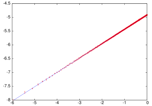
Figure 1: log-log plot of ${\bf E}_{N}[R^{(\rho-\gamma)/\nu}\,1(\theta\leq\Theta\leq\theta+d\theta)]$ vs. $\sin(\theta+d\theta/2)$. The line is the least squares fit to the data.

We first test our second conjecture (21). We divide the range of $\Theta$ into $1800$ equal subintervals and compute ${\bf E}_{N}[R^{(\rho-\gamma)/\nu}\,1(\theta\leq\Theta\leq\theta+d\theta)]$ for each subinterval. We make the approximation

$$\int_{\theta}^{\theta+d\theta}\,\sin(\alpha)^{b-{\overline{b}}}d\alpha\approx\left[\sin(\theta+{d\theta\over 2})\right]^{b-{\overline{b}}}\,d\theta$$

We then do a log-log plot of ${\bf E}_{N}[R^{(\rho-\gamma)/\nu}\,1(\theta\leq\Theta\leq\theta+d\theta)]$ as a function of $\sin(\theta+d\theta/2)$. The result for the $N=1000K$ data is shown in figure 1. The conjecture (21) says that the points should lie on a line. The line shown in the figure is a least squares fit to the data. It has a slope of 0.520655. This should be compared with the conjectured value of $b-{\overline{b}}=25/48=0.52083\overline{3}$.

Next we test our main conjecture (7). In our simulations we generate SAW’s from the uniform probability measure on SAW’s in the half plane with $N$ steps. Let $\gamma$ be the SAW scaled by a factor of $N^{-\nu}$. It is given the weight $R(\gamma)^{(\rho-\gamma)/\rho}$. We apply the conformal map that takes the endpoint of the walk to $i$ and compute the four random variables $X,Y,R$ and $S$ for the transformed walks. Note that we have to normalize by the sum of the weights $R(\gamma)^{(\rho-\gamma)/\rho}$, not by the number of samples generated. Throughout this section we use ${\bf P}_{N}^{\prime}$ to denote this probability measure. It depends on the length of the walks that we use in the simulation, but for large $N$ it should be a good approximation to the ratio in the left side of our first conjecture (7). Our conjecture is that ${\bf P}_{N}^{\prime}$ converges to ${\bf P}^{radial}_{{\mathbb{H}},i}$ as $N\rightarrow\infty$.

The cumulative distribution functions from our simulations are shown in figure 2 along with the exact distributions of these random variables for radial SLE_8/3 that we computed in section 4. There are eight curves in this figure, but the differences between the exact radial SLE_8/3 results and the simulation are too small to be seen in the figure so it appears there are only four curves. The differences between the analytic SLE_8/3 results and the simulations for the four random variables are shown in figures 3 to 6. We plot the differences for $N=200K,500K,1000K$. The most important feature of these plots is the scale on the vertical axis. The full vertical scale on each of the four plots is only $3\times 10^{-4}$. For the most part the deviation of the SAW simulation results from the exact results for SLE_8/3 comes from statistical errors, i.e., from the fact that we cannot run the Monte Carlo simulation forever. Systematic errors from the finite length of the SAW’s can be seen in figures 4 and 5 for values of the random variable just above $1$.

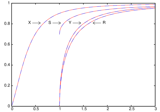
Figure 2: For each of the random variables $X,Y,R$ and $S$ we plot both the cumulative distribution function for radial SLE_8/3 and for the transformed, appropriately weighted SAW. The SLE_8/3 and SAW curves are drawn with dashed lines in different colors. They agree so well that the two dashed lines appear to form a single curve.

N	samples	$b-5/8$	${\overline{b}}-5/48$
100K	566M	-0.0012195299	-0.0003553937
200K	399M	-0.0009095889	-0.0003603211
500K	254M	-0.0004963860	-0.0002366523
1000K	180M	-0.0003692820	-0.0002336083

Table 1: The estimates of $b$ and ${\overline{b}}$ from the SAW simulations. We use four different lengths of walks. The second column gives the number of samples used in millions.

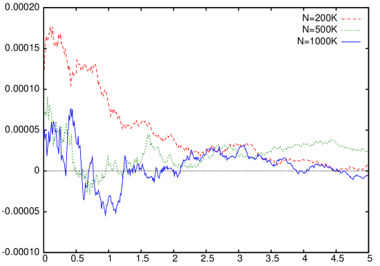
Figure 3: For the random variable $X$ we plot the difference of the cumulative distribution functions for the transformed, appropriately weighted SAW and for radial SLE_8/3.

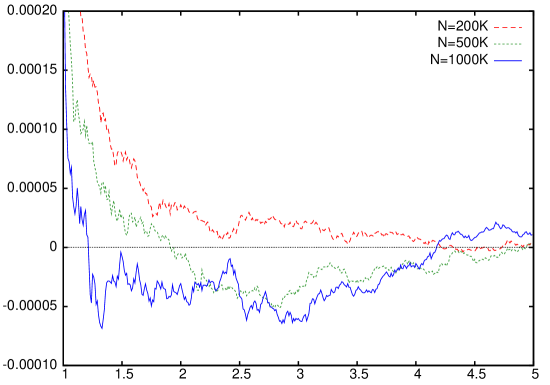
Figure 4: For the random variable $Y$ we plot the difference of the cumulative distribution functions for the transformed, appropriately weighted SAW and for radial SLE_8/3.

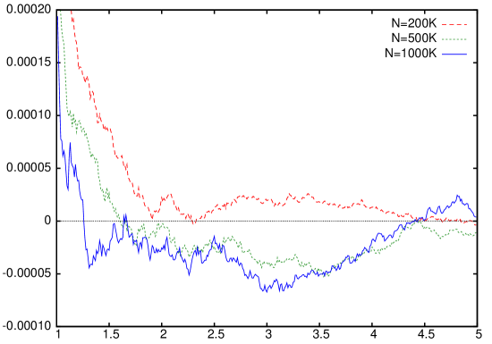
Figure 5: For the random variable $R$ we plot the difference of the cumulative distribution functions for the transformed, appropriately weighted SAW and for radial SLE_8/3.

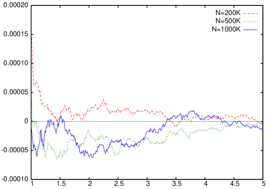
Figure 6: For the random variable $S$ we plot the difference of the cumulative distribution functions for the transformed, appropriately weighted SAW and for radial SLE_8/3.

Let $W$ be one of the random variables $X,Y,R,S$ and $\phi_{w}(z)$ the corresponding conformal map where $w=x,y,r,s$. Taking the $\log$ of (22) we have

$$\log[{\bf P}_{N}^{\prime}(W\leq w)]=b\,\log|\phi_{w}^{\prime}(0)|+{\overline{b}}\,\log|\phi_{w}^{\prime}(i)|$$ (35)

The right side is linear in $b$ and ${\overline{b}}$, so we can do a least squares fit to estimate these two exponents. For each of the four random variables we take a discrete set of values of $w$. For $X$ these values range from $0$ to $5$ by $0.01$. For $Y,R,S$ they range from $1$ to $5$ by $0.01$. Our simulations estimate $\log[{\bf P}_{N}^{\prime}(W\leq w)]$. The calculations in section 4 give $\log|\phi_{w}^{\prime}(0)|$ and $\log|\phi_{w}^{\prime}(i)|$. The results of a least square fit for $b$ and ${\overline{b}}$ using these $1900$ cases of (35) are shown in table 1 for SAW’s with 100K, 200K, 500K and 1000K steps. The values of $b$ and ${\overline{b}}$ are given in terms of their difference with the conjectured values of $b=5/8$ and ${\overline{b}}=5/48$ [16]. Note that values of $b$ and ${\overline{b}}$ we obtain from the simulations are within a few hundredths of a percent of the conjectured values.

6 Conclusions

We have shown how one may obtain radial SLE_8/3 from the scaling limit of the fixed-length SAW in the half-plane. We take a curve from the scaling limit and apply the conformal automorphism of the half-plane that fixes the origin and maps the endpoint of the curve to $i$. This transformation by itself does not transform the fixed-length SAW into radial SLE_8/3 from from $0$ to $i$. We must also change the probability measure by weighting each curve from the fixed-length scaling limit by $R^{p}$ where $R$ is the distance of the endpoint of the curve to the origin. The power $p$ is conjectured to be $(\rho-\gamma)/\nu=-61/48$.

Our heuristic derivation of the conjectured relationship of the fixed-length SAW to radial SLE_8/3 is further supported by Monte Carlo simulations of the SAW. In particular, we computed estimates of the scaling exponents $b$ and ${\overline{b}}$ and found values that agree with the conjectured values within a few hundredths of a percent. Our simulations also gave a partial test of predictions of the SLE partition function (5) for the SAW in the half-plane with arbitrary length.

An obvious open problem is to prove the relationship between the fixed-length SAW and radial SLE_8/3. Given the near total absence of rigorous results on the two-dimensional SAW, progress on this problem would be a major breakthrough.

Acknowledgments: Oded Schramm’s suggestion to test if simply applying the conformal map to the fixed-length SAW would give radial SLE_8/3 stimulated the author’s interest in this problem. The author has also benefited from discussions with Greg Lawler and Wendelin Werner. This research was supported in part by the National Science Foundation under grant DMS -0758649.

References

- [1] M. Bauer, D. Bernard, 2D growth processes: SLE and Loewner chains, Phys. Rep. 432, 115-221 (2006). Archived as arXiv:math-ph/0602049v1.
- [2] J. Cardy, SLE for theoretical physicists, Ann. Physics 318, 81-118 (2005). Archived as arXiv:cond-mat/0503313v2 [cond-mat.stat-mech].
- [3] N. Clisby, Efficient implementation of the pivot algorithm for self-avoiding walks, J. Statist. Phys. 140, 349-392 (2010). Archived as arXiv:1005.1444v1 [cond-mat.stat-mech].
- [4] H. Duminil-Copin,S. Smirnov, The connective constant of the honeycomb lattice equals . Preprint, 2010. Archived arXiv:1007.0575v1 [math-ph].
- [5] B. Dyhr, M. Gilbert, T. Kennedy, G. Lawler, S. Passon, The self-avoiding walk in a strip. Preprint (2010). Archived as arXiv:1008.4321v1 [math.PR].
- [6] P.J. Flory, The configuration of a real polymer chain, J. Chem. Phys. 17, 303-310 (1949).
- [7] W. Kager, B. Nienhuis, A guide to stochastic Loewner evolution and its applications, J. Statist. Phys. 115, 1149-1229 (2004). Archived as arXiv:math-ph/0312056v3.
- [8] T. Kennedy, A faster implementation of the pivot algorithm for self-avoiding walks, J. Stat. Phys. 106, 407-429 (2002). Archived as arXiv:cond-mat/0109308v1.
- [9] T. Kennedy, Monte Carlo tests of SLE predictions for 2D self-avoiding walks, Phys. Rev. Lett. 88, 130601 (2002). Archived as arXiv:math/0112246v1 [math.PR].
- [10] T. Kennedy, Conformal invariance and stochastic Loewner evolution predictions for the 2D self-avoiding walk - Monte Carlo tests, J. Stat. Phys. 114, 51–78 (2004). Archived as arXiv:math/0207231v2 [math.PR].
- [11] H. Kesten, On the number of self-avoiding walks, J. Math. Phys 4, 960-969 (1963).
- [12] H. Kesten, On the number of self-avoiding walks II, J. Math. Phys 5, 1128-1137 (1964).
- [13] G. Lawler, Partition functions, loop measure, and versions of SLE. J. Statist. Phys. 134, 813-837 (2009).
- [14] G. Lawler, Conformally Invariant Processes in the Plane. American Mathematical Society (2005).
- [15] G. Lawler, Schramm-Loewner evolution, in Statistical Mechanics, S. Sheffield and T. Spencer, ed., IAS/Park City Mathematical Series, AMS, 231-295 (2009). Archived as arXiv:0712.3256v1 [math.PR].
- [16] G. Lawler, O. Schramm, and W. Werner, On the scaling limit of planar self-avoiding walk, Fractal Geometry and Applications: a Jubilee of Benoit Mandelbrot, Part 2, 339–364, Proc. Sympos. Pure Math. 72, Amer. Math. Soc., Providence, RI, 2004. Archived as arXiv:math/0204277v2 [math.PR].
- [17] G. Lawler, O. Schramm, W.Werner, Conformal restriction: the chordal case, J. Amer. Math. Soc. 16, 917-955 (2003). Archived as arXiv:math/0209343v2 [math.PR].
- [18] N. Madras and G. Slade, The Self-Avoiding Walk. Birkhäuser (1996).
- [19] B. Nienhuis, Exact critical exponents for the models in two dimensions, Phys. Rev. Lett. 49 1062-1065 (1982).
- [20] O. Schramm, Scaling limits of loop-erased random walks and uniform spanning trees, Israel J. Math. 118, 221-288 (2000). arXiv:math/9904022v2 [math.PR].
- [21] O. Schramm, private communication, November, 2002.
- [22] W. Werner, Random planar curves and Schramm-Loewner evolutions, Ecole d’Eté de Probabilités de Saint-Flour XXXII - 2002, Lecture Notes in Mathematics 1840, Springer-Verlag, 107–195 (2004). Archived as arXiv:math/0303354v1 [math.PR].