The conformal window on the lattice

Abstract:

Lattice simulations can play an important role in the study of dynamical electroweak symmetry breaking by providing quantitative results on the nonperturbative dynamics of candidate theories. For this programme to succeed, it is crucial to identify the questions that are relevant for phenomenology, and develop the tools that will provide robust answers to these questions. The existence of a conformal window for nonsupersymmetric gauge theories, and its characterization, is one of the phenomenologically important problems that can be studied on the lattice. We summarize the recent results from studies of IR fixed points by numerical simulations, discuss their current limitations, and analyze the future perspectives.

1 Motivations and aims

Theories that are asymptotically free at high energies, and have an infrared fixed point (IRFP) in the renormalization group (RG) flow of their couplings are said to be inside the “conformal window”. The typical running of the coupling, with its limiting value $g^{*}$ at small energies, is shown in Fig. 1. The existence of a conformal window has been studied analytically for supersymmetric theories, see e.g. Ref. [1] for a review. Quantitative analytical studies of the IR regime for the non-supersymmetric cases are more difficult, due to a lack of adequate tools to investigate the nonperturbative dynamics of gauge theories. Nevertheless interesting results have appeared in recent years, see e.g. Refs. [2, 3, 4, 5] for a summary. Besides its field-theoretical interest, the existence of a conformal window has important consequences for building models of physics beyond the standard model (BSM) that are based on strongly-interacting theories.

Figure 1: Running of the coupling as a function of the energy scale for a theory with an IRFP. At low energies the coupling flows to a fixed-point value $g^{*}$, while the high energy behaviour is the usual one expected for asymptotically free theories. The scale $\Lambda_{\mathrm{U}}$ corresponds approximately to the energy where the running starts to be dictated by asymptotic freedom. The dashed curve at low energies shows the running of the coupling when a fermionic mass term is switched on.

Models of dynamical electroweak symmetry breaking (DEWSB) provide elegant realizations of the mechanism responsible for the breaking of electroweak symmetry down to electromagnetism, by means of the vacuum expectation value of a fermion bilinear, see Ref. [6] for a review and a list of references. In the simplest versions of DEWSB, the fermion condensate is produced by the strong dynamics of some new asymptotically free non-abelian gauge theory. The new gauge group is usually called “technicolor” (TC) [7, 8]. The massless fermions coupled to this new gauge field are called “technifermions”; they transform under some representation of the new gauge group, and their left-handed components are weak doublets, so that their condensate breaks electroweak symmetry in the standard model (SM). The technifermion condensate also breaks the global chiral symmetry of the technicolor theory, in analogy with chiral symmetry breaking in QCD, and therefore implies the existence of massless “technipions”. The number and the dynamics of technipions depend on the details of the technicolor model. Three of these technipions are “Higgsed” and become the longitudinal components of the $W$ and $Z$ bosons. As a result, the latter acquire a mass proportional to the technipion decay constant, and therefore $F_{T}\sim v\sim 250~{}\mathrm{GeV}$, where $v$ denotes the Higgs condensate in the SM. This constraint sets the typical scale of the technihadronic spectrum, $\Lambda_{\mathrm{TC}}$. The rest of the technihadron spectrum depends on the specific theory that is selected to mediate the new strong force. Being able to compute in the strongly-interacting regime of the technicolor theories is the main ingredient to understand this mechanism.

Lattice simulations are a prime tool to investigate nonperturbative physics from first principles. However numerical studies will play an important role in BSM studies only if we are able to identify the questions that are relevant in order to achieve a quantitative understanding of DEWSB. In this introduction we briefly review some of the problems that technicolor model building is confronted to, and analyze the possibility to use numerical results to make progress in this area.

Constraints on technicolor.

While technicolor provides a natural way to generate $W$ and $Z$ masses, additional interactions must be introduced in order to describe the SM flavor sector. A scenario that has been extensively studied involves “extended technicolor” gauge interactions (ETC) [9, 10]. The ETC gauge bosons couple to both the SM fermions and the technifermions. At some energy $M_{\mathrm{ETC}}$, larger than the TC scale, the extended gauge symmetry is then broken down to the residual TC gauge symmetry, which remains intact. As a result, interactions between the technifermions and the ordinary standard model fermions are generated at low-energies. We have so far introduced two new sectors, a TC one and an ETC one. Their connections and the energy scales involved are summarized in Fig. 2. Note that below the ETC scale the TC theory and the flavor sector of the SM are decoupled.

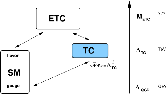
Figure 2: A schematic representation of the technicolor (TC) and extended technicolor (ETC) theories, and their connections with the standard model (SM). The interactions are characterized by different scales, indicated on the right. Bounds on the ETC scale $M_{\mathrm{ETC}}$ are set by SM precision measurements.

In current simulations, only the TC sector is simulated on the lattice. At energies of the order of the TC scale, the ETC-mediated interactions are described by the effective lagrangian obtained when the heavy ETC degrees of freedom are integrated out. This lagrangian includes four-fermion operators, whose couplings are suppressed by inverse powers of the ETC scale. These are dimension-six operators involving technifermions and SM fermions; denoting the SM and TC fermion fields by $\psi(x)$ and $Q(x)$ respectively, the terms that are relevant for our discussion can be schematically written as:

$$\frac{1}{M_{\mathrm{ETC}}^{2}}\bar{Q}(x)Q(x)\bar{\psi}(x)\psi(x)\,,$$ (1)

$$\frac{1}{M_{\mathrm{ETC}}^{2}}\bar{\psi}(x)\psi(x)\bar{\psi}(x)\psi(x)\,,$$ (2)

where for simplicity we have suppressed the flavor, color and spin indices.

Eq. (1) shows that a technifermion condensate $\langle\bar{Q}Q\rangle$ generates a mass term for the SM fermions. It is worthwhile to recall here that the quark masses in the SM are defined in a given renormalization scheme and at a given scale $\mu$, see e.g. the review in Ref. [6]. When the fermion masses are generated via an ETC theory, this dependence is reflected in the scheme and scale dependence of the technifermion condensate. We are going to follow the convention used in the PDG and always refer to the quark masses in the $\overline{\mathrm{MS}}$ scheme. However it should be clear that this choice is arbitrary, and that it is possible to convert from one scheme to the other. Below the scale $M_{\mathrm{ETC}}$ the technicolor and the flavor sectors decouple, and therefore the running of the quark masses is simply given by the QCD logarithmic evolution, which we neglect here. In an ETC scenario, the SM fermion masses are therefore set by the value of the technifermion condensate in the $\overline{\mathrm{MS}}$ scheme at the scale $M_{\mathrm{ETC}}$:

$$m(M_{\mathrm{ETC}})=\frac{1}{{}_{\Lambda^{2}_{\mathrm{ETC}}}}\left.\langle\bar{Q}Q\rangle\right|_{M_{\mathrm{ETC}}}=\frac{1}{{}_{\Lambda^{2}_{\mathrm{ETC}}}}\exp\left[\int_{\Lambda_{\mathrm{TC}}}^{M_{\mathrm{ETC}}}\frac{d\mu}{\mu}\gamma(\mu)\right]\left.\langle\bar{Q}Q\rangle\right|_{\Lambda_{\mathrm{TC}}}\,,$$ (3)

where $\gamma$ is the mass anomalous dimension of the technicolor theory in this scheme, and the second equality shows explicitly the evolution of the chiral condensate.

On the other hand, ETC interactions in Eq. (2) include flavor changing neutral currents (FCNC), which would result in sizeable contributions to $K$ and $D$ mixing. As noted long ago [9], the experimental limits on such contributions imply a lower bound on the ETC scale. For instance the ETC scale associated with the generation of the strange mass should be larger than $10^{3}~{}\mathrm{TeV}$, unless some fine-tuned mechanism is in place. As a consequence of this large value of $M_{\mathrm{ETC}}$, heavy quark masses can be generated only if the techniquark condensate is enhanced with respect to the naive value obtained by rescaling QCD. A detailed discussion of the fermion mass generation in ETC models can be found in Ref. [11]. Recent summaries on technicolor and the constraints imposed by current measurements can be found in Refs. [2, 12, 13].

It has been suggested that “walking” theories, i.e. theories where the RG evolution is very slow, could produce the required enhancement of the condensate [14, 15, 16, 17, 18, 19, 20]. This is illustrated in Eq. (3): if the couplings are approximately constant as the energy scale varies, the integral of the anomalous dimension yields a power enhancement:

$$\left.\langle\bar{Q}Q\rangle\right|_{M_{\mathrm{ETC}}}=\left(\frac{M_{\mathrm{ETC}}}{\Lambda_{\mathrm{TC}}}\right)^{\gamma}\left.\langle\bar{Q}Q\rangle\right|_{\Lambda_{\mathrm{TC}}}\,.$$ (4)

For comparison note that, in a QCD-like theory, the condensate at the higher scale is of the order of $\left\langle\bar{Q}Q\rangle\right|_{\Lambda_{\mathrm{TC}}}$ up to logarithmic corrections. For a sufficiently large value of $\gamma$, the factor in Eq. (4) can yield large quark masses and hence ease the tension between technicolor and the flavor sector of the SM. Recent analyses suggest that $\gamma>1$ is needed to avoid a fine-tuned ETC sector [21], while unitarity constraints imply that $\gamma<2$ [22]. For a strongly-coupled theory, the value of $\gamma$ can only be computed by nonperturbative methods.

Furthermore “walking” theories are expected to ease the tension between TC and the constraints from electroweak precision measurements [23, 24, 25].

A lucid list of questions that need to be addressed in order to build a phenomenologically successful model of DEWSB is presented in Ref. [26].

It is important to recall that the rate at which the coupling constants evolve, and the corresponding power enhancement, depend on the renormalization scheme, and therefore the definition of “walking” needs to be qualified better. The existence of an IRFP, i.e. a zero of the beta functions for the couplings at small energy scales, is independent of the scheme. It describes the physical properties of theories that are scale-invariant at large distances, where the field correlators have power-like behaviours characterized by the anomalous dimensions of the fields . A concise description of the scheme dependent features of IRFPs is presented in Ref. [27].

The conformal window.

In the absence of fermionic matter fields, SU(N) gauge theories are asymptotically free. The running of the gauge coupling $g$ is encoded in the beta function, which can be computed in perturbation theory close to the Gaussian fixed point $g=0$:

$$\mu\frac{d}{d\mu}g=\beta(g)=-\beta_{0}g^{3}-\beta_{1}g^{5}+\ldots\,.$$ (5)

At one-loop in perturbation theory the effect of the fermion fields can be read from the first coefficient

$$\beta_{0}=\frac{1}{(4\pi)^{2}}\left[\frac{11}{3}C_{2}(A)-\frac{4}{3}T_{R}n_{f}\right]\,,$$ (6)

where $C_{2}(R)$ and $T_{R}$ denote respectively the quadratic Casimir and the normalization of the generators in the representation $R$. The coefficient $C_{2}(A)$ originates from the gluons being in the adjoint representation of the gauge group, and $n_{f}$ counts the number of Dirac fermions in the theory. At one loop the dependence on the fermionic representation is entirely encoded in the factor $T_{R}$. In discussing perturbative results, we use here the same conventions introduced in Ref. [28]. As the number of fermion fields is increased, $\beta_{0}$ changes sign and asymptotic freedom is lost. We shall denote by $n_{f,\mathrm{up}}$ the number of fermions above which asymptotic freedom is lost, clearly such a number depends on the gauge group and the fermionic representation.

At higher orders in perturbation theory the fermionic contribution to the running of the coupling has the potential to generate a non-trivial zero of the beta function before asymptotic freedom is lost. This is signalled in perturbation theory by a change of sign of the coefficient $\beta_{1}$. We shall denote by $n_{f,\mathrm{lo}}$ the number of fermions above which the theory exhibits an IRFP. In this case the theory becomes scale-invariant at large distances, while the short-distance behaviour is still the one dictated by asymptotic freedom. As a consequence of scale invariance at large distances, the theory cannot be in a confining phase and chiral symmetry remains unbroken. The long-distance dynamics is governed by the IRFP’s critical exponents, which determine the scaling laws in the vicinity of the fixed point. The range of values $n_{f,\mathrm{lo}}<n_{f}<n_{f,\mathrm{up}}$ is known as the “conformal window”. The Banks-Zaks theories [29, 30], where $N_{c}$ and $n_{f}$ are arranged such that the critical coupling $g^{*}\ll 1$, provide one working example of theories within the conformal window that can be analysed in perturbation theory.

Theories near the edge of the conformal window (e.g. $n_{f}\lesssim n_{f,\mathrm{lo}}$) have been recently put forward as candidate walking theories [31]. Alternative scenarios start from a theory inside the conformal window, and deform the theory away from conformality by perturbing it with operators that are relevant in the IR regime [32], see also Refs. [33, 34]. In both cases, the starting point is being able to identify the conformal window, i.e. to be able to identify the existence of a fixed point, and to compute the critical exponents that characterize the relevant directions of the RG flow. We shall concentrate on this specific problem in this review.

Informations about the existence of IRFPs in nonsupersymmetric gauge theories can be obtained by analytical methods like e.g. the solution of the truncated Schwinger-Dyson equation [35, 36, 37, 38], or the usage of conjectures about the nonperturbative behaviour of quantum field theories [39]. This information is valuable to guide the numerical investigations, but robust results ultimately need investigations that rely on first principles; besides the lattice studies discussed below, interesting analytical results for the anomalous dimensions in a CFT have been obtained in Ref. [40] from first principles.

Lattice evidence.

Having set the task to identify the existence of IR fixed points, we need to spell out clearly what are the observables that can be evaluated by Monte Carlo methods, and what are the systematic errors that need to be kept under control in order to draw meaningful conclusions from the lattice data.

The tools that have been developed for the numerical studies of QCD can be adapted to this new class of theories, yielding new and interesting informations. These tools are reviewed in Sect. 2 below.

In order to perform a lattice study, a particular theory has to be selected and simulated. Analytical results can help in selecting candidate theories inside the conformal window. However the lack of robust analytical results means that there is no guarantee of being inside (or near) the conformal window before simulations are performed. As a consequence, numerical tools developed for these studies need to provide:

• flexibility; so that the same codebase can be used to simulate more than just one theory.

• efficiency; so that simulations are reasonably fast. At this stage, it is important to find the right balance between optimization and flexibility.

• a wide range of observables; so that robust conclusions can be drawn, based on more than one observation.

• detailed numerical benchmarks, so that the algorithmic issues can be clearly identified, and distinguished from the physically meaningful results. In my opinion these algorithmic studies have not yet reached the maturity of their QCD counterparts.

A few candidate theories have been studied recently, chosen according to the conjectured boundaries of the conformal window for SU(N) gauge theories with fermions in the fundamental, adjoint or two-index representations. These boundaries have been summarized in Ref. [2], whence the plot in Fig. 3 is extracted. As shown in this plot, theories with fermions in higher dimensional representations of the gauge group are expected to develop a fixed point for relatively small numbers of flavors. Recent studies have focused on theories that are close to the lower edge of the conformal window: SU(3) with $n_{f}=16,12,10,9,8,6$ flavors in the fundamental representation, SU(2) with $n_{f}=6$ flavors in the fundamental, SU(2) with $n_{f}=2$ flavors in the adjoint representation, and SU(3) with $n_{f}=2$ flavors in the two-index symmetric (sextet) representation. At these early stages of the nonperturbative studies of the conformal window it is important to try to identify a paradigm to guide the numerical investigations, rather than trying to get exhaustive results on one specific theory.

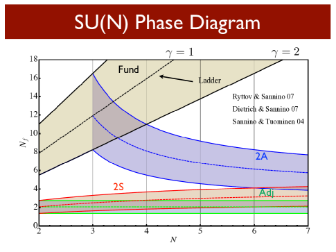
Figure 3: Boundaries of the conformal window for SU(N) gauge theories with $n_{f}$ species of Dirac fermions. The four bands represent respectively fermions in the fundamental (Fund), adjoint (A) and two-index symmetric and antisymmetric (2S,2A) representations. The upper limit of each band corresponds to the number of flavors where asymptotic freedom is lost, as obtained from one-loop perturbative computations. The lower limit of each band yields the number of flavors above which the theories develop an IR fixed point. The location of these lower limits relies upon assumptions about the nonperturbative dynamics of the theories. Lattice simulations can provide first-principle evidence in favour (or against) this picture, and compute the critical exponents that characterize the fixed points. Figure courtesy of F. Sannino.

2 Tools

Numerical tools that were originally designed for investigating lattice QCD have been used in order to identify the existence of IRFPs. We describe briefly the main ideas, the observables that are used in the different approaches, and their expected behaviour in the presence of an IRFP. For each case we try to emphasize the sources of systematic errors that need to be kept under control in order to draw robust conclusions from numerical data.

2.1 Phase structure of the lattice theories.

Lattice simulations are performed by discretizing the action of a given theory on a Euclidean space-time lattice. At weak coupling the RG flow can be computed perturbatively, and the relevant parameters are easily identified. For an asymptotically-free gauge theory, $g=0$ is an UV fixed point that defines the usual continuum limit of the lattice theory. The IRFP that we are seeking is a fixed point on the massless renormalized trajectory that originates from the continuum limit. As the bare coupling is increased, the lattice theory may have a complicated phase structure, with new fixed points appearing, which are not necessarily related to the continuum limit.

In particular there can be bulk phase transitions in the lattice theory at strong coupling. These are lattice artefacts and can obscure the continuum physics that we are interested in. Mapping the phase structure of the lattice theory is important in order to be able to identify the genuine features of the continuum limit.

Finite volume effects also play an important role in determining the long-distance behaviour of a gauge theory. The inverse size of the lattice $1/L$ is a relevant coupling in the IR, which introduces an explicit length scale: we can only probe energies above $1/L$ when performing lattice simulations in a finite box, while the largest scaling factor that we can probe in a simulation is $s_{\mathrm{max}}=L/a$.

There are two potential effects to take into account. On the one hand, as the box size is decreased, the IR cutoff can potentially change the behaviour of the gauge theory and drive the theory into different phases, characterized by the breaking of centre symmetries [41, 42]. It is important to study the impact of these transitions on the measured observables. On the other hand, even when the box is large enough and the system is in the correct phase, $1/L$ determines the size of the scaling violations. These can be readily included in scaling laws determined from RG analyses [43, 44, 45, 46, 47].

2.2 Spectral studies

Informations about the mass spectrum and the decay constants of a given gauge theory, can be obtained from the numerical analysis of two-point correlators, using the standard techniques developed for QCD.

Simulations are performed at a finite value of the mass, and in a finite volume. Both these quantities break conformal invariance at large distances. The signatures of an IRFP in this framework are the scaling laws of physical observables as functions of the mass and volume, as it is often the case when studying critical phenomena. Using the scaling behaviour of lattice observables to identify IRFP was proposed in Refs. [48, 49, 43, 50]. Scaling laws are derived using the RG equations for field correlators [43, 50]. A detailed analysis of the scaling of lattice observables was discussed in Refs. [46, 47]. Scaling laws in the vicinity of a fixed point were already considered in searches for UV fixed points in lower-dimensional field theories. For a summary of results in the case of three-dimensional four-fermi theories, see e.g. Ref. [51] and references therein.

The masses of the states in the technihadron spectrum scale as:

$$M_{H}\sim m^{1/y_{m}}\,,$$ (7)

where $y_{m}=1+\gamma_{*}$ is the critical exponent associated to the fermion mass, and $\gamma_{*}$ is the (scheme-independent) value of the anomalous dimension at the fixed point.

A generic operator $O$ with appropriate quantum numbers couples to the states of the theory with strength denoted $G_{H}$ for a scalar state, and $F_{V}$ for a vector one. The scaling of these couplings, which are related to the decay constant of the state $H$, can also be derived from the scaling behaviour of two-point correlators. Following the notation introduced in Ref. [46] the scaling behaviour of the decay constants can be written as:

$$G\sim m^{\eta_{G}}\,,~{}~{}~{}~{}F\sim m^{\eta_{F}}\,,$$ (8)

with the exponents summarized in Tab. 1. Note that the scaling relations hold for any state in the spectrum. In particular for the pseudoscalar meson states, they yield a modified Banks-Casher relation. Scaling laws in the vicinity of a fixed point have also been discussed in the context of the functional RG, see e.g. Ref. [52, 53].

$O$	def	$\langle 0|O|J^{\mathrm{P(C)}}(p)\rangle$	$J^{\mathrm{P(C)}}$	$\Delta_{O}$	$\eta_{G[F]}$
$S$	$\bar{q}q$	$G_{S}$	$0^{++}$	$3-\gamma_{*}$	$(2-\gamma_{*})/y_{m}$
$S^{a}$	$\bar{q}\lambda^{a}q$	$G_{S^{a}}$	$0^{+}$	$3-\gamma_{*}$	$(2-\gamma_{*})/y_{m}$
$P^{a}$	$\bar{q}i\gamma_{5}q$	$G_{P^{a}}$	$0^{-}$	$3-\gamma_{*}$	$(2-\gamma_{*})/y_{m}$
$V$	$\bar{q}\gamma_{\mu}q$	$\epsilon_{\mu}(p)M_{V}F_{V}$	$1^{--}$	$3$	$1/y_{m}$
$V^{a}$	$\bar{q}\gamma_{\mu}\lambda^{a}q$	$\epsilon_{\mu}(p)M_{V}F_{V^{a}}$	$1^{-}$	$3$	$1/y_{m}$
$A^{a}$	$\bar{q}\gamma_{\mu}\gamma_{5}\lambda^{a}q$	$\epsilon_{\mu}(p)M_{A}F_{A^{a}}$	$1^{+}$	$3$	$1/y_{m}$
		$ip_{\mu}F_{P^{a}}$	$0^{-}$	$3$	$1/y_{m}$

Table 1: Scaling laws, $G[F]\sim m^{\eta_{G[F]}}$ for decay constants. The symbol $y_{m}\equiv 1+\gamma_{*}$ denotes the scaling dimension of the mass and $\Delta_{O}=d_{O}+\gamma_{O}$ is the scaling dimension of the operator $O$. The symbol $a$ denotes the adjoint flavour index, and $\lambda^{a}$ are the generators normalized as $\mathrm{tr}[\lambda^{a}\lambda^{b}]=2\delta^{ab}$. No such simple expression exists for the axial singlet current because of the chiral anomaly [46].

It is important to bear in mind that scaling laws are asymptotic formulae that are obtained by linearizing the RG equations in a neighbourhood of the fixed point at $m=0$ and $1/L=0$. As the system moves towards larger values of $m$ and $1/L$, the corrections to scaling become important and eventually obscure the power-law scaling dictated by the IRFP. The critical exponents can be extracted from the power-law scaling of the spectrum only from simulations at small mass.

The distinctive feature in the spectrum of an IR-conformal theory is the lack of spontaneous chiral symmetry breaking. As a consequence, there are no Goldstone bosons in the theory. As the fermion mass is sent to zero all states in the spectrum become massless, see e.g. Ref. [54] for a realization of this scenario. This is at odds with the chirally-broken scenario, where there is a parametric separation between the pseudoscalar Goldstone bosons and the rest of the massive spectrum. Any effective theory that describes the low-energy dynamics of an IR-conformal system must take all the light degrees of freedom into account.

As simulations move to smaller fermion masses, the physical size of the lattice must be increased in order to avoid finite-size effects. In particular a chirally broken theory at small mass and fixed physical volume can enter the so-called $\delta$-regime, where the spectrum is determined by the rotator states of the chiral condensate [55]. This regime corresponds to $L_{t}\gg L_{s}$, $FL_{s}>1$, and $ML_{s}\ll 1$; the spectrum of the lowest states no longer scales as expected for the Goldstone bosons of a chirally broken theory. In this case deviations from the GMOR scaling are not a signal of restoration of chiral symmetry. Similarly if $L_{t}\sim L_{s}$ the system will be driven in the $\epsilon$ regime, which can be seen as the high-temperature limit of the $\delta$-regime. Great care must be exercised in the interpretation of lattice data, as these finite size effects can easily be mistaken for signals of conformal behaviour. This has been clearly pointed out in Ref. [56]. The $\delta$ regime can be distinguished from a conformal one if the power-law scaling corresponding to the latter is observed.

Last but not least, it is important to verify that the simulated masses do not correspond to the “heavy quark” limit of a chirally broken theory. This can be achieved by comparing the mesonic and gluonic sectors of the spectrum as discussed in the next section, where we report the numerical results.

2.3 SF studies

The nonperturbative running of the gauge coupling and fermion mass can be studied using the Schrödinger functional scheme [57, 58]. The running coupling $\overline{g}^{2}$ at the scale $1/L$ is defined on a hypercubic lattice of size $L$, with boundary conditions chosen to impose a background chromoelectric field, which depends on a parameter $\eta$. The renormalized coupling is defined as a measure of the response of the system to changes in the background chromoelectric field:

$$\overline{g}^{2}=k\left<\frac{\partial S}{\partial\eta}\right>^{-1}\,,$$ (9)

where $S$ is the action of the Schrödinger functional, and the constant $k$ is chosen such that $\overline{g}^{2}=g_{0}^{2}$ to leading order in perturbation theory. Eq. (9) defines a nonperturbative coupling, which depends on only one scale, the size of the system $L$, and can be evaluated numerically.

To measure the running of the quark mass, we calculate the pseudoscalar density renormalisation constant $Z_{P}$. Following Ref. [59], $Z_{P}$ is defined by:

$$Z_{P}(L)=\sqrt{3f_{1}}/f_{P}(L/2)\,,$$ (10)

where $f_{1}$ and $f_{P}$ are the correlation functions involving the boundary fermion fields $\zeta$ and $\overline{\zeta}$:

$$f_{1} = -1/12L^{6}\int d^{3}u\,d^{3}v\,d^{3}y\,d^{3}z\,\langle\overline{\zeta}^{\prime}(u)\gamma_{5}\tau^{a}{\zeta}^{\prime}(v)\overline{\zeta}(y)\gamma_{5}\tau^{a}\zeta(z)\rangle\,,$$ (11)

$$f_{P}(x_{0}) = -1/12\int d^{3}y\,d^{3}z\,\langle\overline{\psi}(x_{0})\gamma_{5}\tau^{a}\psi(x_{0})\overline{\zeta}(y)\gamma_{5}\tau^{a}\zeta(z)\rangle\,.$$ (12)

For the details of the Schrödinger functional setup we refer the reader to the original publications.

The running of the coupling as the scale is varied by a factor $s$ is encoded in the step scaling function $\sigma(u,s)$ as

$$\Sigma(u,s,a/L) = \left.\overline{g}^{2}(g_{0},sL/a)\right|_{\overline{g}^{2}(g_{0},L/a)=u}\,,$$ (13)

$$\sigma(u,s) = \lim_{a/L\to 0}\Sigma(u,s,a/L)\,,$$ (14)

as described in Ref. [58]. The function $\sigma(u,s)$ is the continuum extrapolation of $\Sigma(u,s,a/L)$ which is obtained from numerical simulations at various $a/L$ values and fixed $u$. The step scaling function encodes the same information as the $\beta$ function. The relation between the two functions for a generic rescaling of lengths by a factor $s$ is given by:

$$-2\log s=\int_{u}^{\sigma(u,s)}\frac{dx}{\sqrt{x}\beta(\sqrt{x})}\,.$$ (15)

The step scaling function can be computed at a given order in perturbation theory by using the analytic expression for the perturbative $\beta$ function, and solving Eq. (15) for $\sigma(u,s)$. It can be seen from the definition of $\sigma(u,s)$ in Eq. (14) that an IRFP corresponds to $\sigma(u,s)=u$.

The lattice step scaling function for the mass is defined as:

$$\Sigma_{P}(u,s,a/L)=\left.{\frac{Z_{P}(g_{0},sL/a)}{Z_{P}(g_{0},L/a)}}\right|_{\overline{g}^{2}(L)=u}\,;$$ (16)

the mass step scaling function in the continuum limit, $\sigma_{P}(u,s)$, is given by:

$$\sigma_{P}(u,s)=\lim_{a\to 0}\Sigma_{P}(u,s,a/L)\,.$$ (17)

The mass step scaling function is related to the mass anomalous dimension (see e.g. Ref. [60]):

$$\sigma_{P}(u)=\left(\frac{u}{\sigma(u)}\right)^{(d_{0}/(2\beta_{0}))}\exp\left[\int_{\sqrt{u}}^{\sqrt{\sigma(u)}}dx\left(\frac{\gamma(x)}{\beta(x)}-\frac{d_{0}}{\beta_{0}x}\right)\right]\,.$$ (18)

In the vicinity of an IRFP the relation between $\sigma_{P}$ and $\gamma$ simplifies:

$$\int_{\overline{m}(\mu)}^{\overline{m}(\mu/s)}\frac{dm}{m}=-\gamma_{*}\int_{\mu}^{\mu/s}\frac{dq}{q}\,,$$ (19)

and hence:

$$\log\left|\sigma_{P}(s,u)\right|=-\gamma_{*}\log s\,.$$ (20)

We can therefore define an estimator

$$\hat{\gamma}(u)=-\frac{\log\left|\sigma_{P}(u,s)\right|}{\log\left|s\right|}\,,$$ (21)

which yields the value of the anomalous dimension at the fixed point. Away from the fixed point $\hat{\gamma}$ will deviate from the anomalous dimension, with the discrepancy becoming larger as the anomalous dimension develops a sizeable dependence on the energy scale.

The step scaling functions need to be extrapolated to the continuum limit in order to disentangle the running of the couplings from the lattice artefacts that affect the measured observables. This extrapolation is very delicate for $\sigma(u,s)$. In the vicinity of a fixed point the running is by definition very slow. Therefore a very high accuracy in the extrapolation is needed in order to resolve the physically meaningful signal. The systematic uncertainties make it difficult to locate the value of the critical coupling with sufficient accuracy. In the next section, we shall discuss in more detail the propagation of errors and their impact on the physically interesting results.

2.4 Potential schemes

Finally the running of the coupling can be studied by defining a nonperturbative coupling from the potential between static charges computed numerically [61].

The coupling is defined as:

$$g_{w}^{2}(L_{0},R/L_{0},a/L_{0})=\frac{1}{k}(R/a)^{2}\chi(R/a,L_{0}/a)\,,$$ (22)

where $\chi$ is a Creutz ratio, $L_{0}$ is the size of the lattice, and $R$ is the size of the Wilson loops used to construct the Creutz ratios. The size of the lattice $L_{0}$ sets the scale at which the coupling is defined, while the ratio $R/L_{0}$ defines the renormalization scheme.

A step scaling function can be defined in close analogy to the one defined for the Schrödinger functional:

$$\Sigma_{w}(u,R/L_{0},a/L_{0})=g_{w}^{2}(bL_{0},R/L_{0},a/L_{0})\,,$$ (23)

$$u=g_{w}^{2}(L_{0},R/L_{0},a/L_{0})\,,$$ (24)

$$\sigma_{w}(u)=\lim_{a\to 0}\Sigma_{w}(u,R/L_{0},a/L_{0})\,.$$ (25)

Once again the extrapolation to the continuum limit in Eq. (25) is necessary in order to avoid contaminations from lattice artefacts.

Ref. [62] presents a variation on the same theme. The potential between static charges is measured by lattice simulations, and is compared with the results obtained from integrating the running coupling:

$$V(R)-V(R_{0})=C_{s}(R)\int_{R_{0}}^{R}dR^{\prime}\,\frac{\alpha(R^{\prime})}{R^{\prime 2}}\,,$$ (26)

where the perturbative expansion is used as an input for $\alpha(R)$ in the integral. This method allows one to compare the nonperturbative running with the perturbative expectation.

2.5 MCRG

Monte Carlo Renormalization Group (MCRG) methods were developed in order to study the coupling flow in both spin and gauge models. In particular, the 2-lattice matching has proved to be useful in pure Yang-Mills theories [63, 64, 65].

The basic idea is to follow the RG flow of the bare couplings under blocking transformations that integrate out the UV degrees of freedom. With each blocking step, changing the scale by a factor $s$, the flow drives the couplings towards a lower-dimensional manifold, whose dimension is given by the number of relevant couplings. The distance from this manifold goes as a power of $s$.

2.5.1 Two-lattice matching procedure

Let us consider first for simplicity a theory that has only one relevant parameter flowing out from an UV fixed point; this is the common situation in pure gauge theories. In this case the RG trajectories converge towards a one-dimensional renormalized trajectory (RT). Starting from a value $g$ of the bare coupling at the cutoff scale, after $n$ steps the Wilsonian action is described by some point in parameter space, for a sufficiently large $n$ this point is close to the RT. This is represented by the circles and the blue curve in Fig. 4, for $n=4$ steps of blocking starting from the value $g=K$. This point is matched by the point $g^{\prime}=K^{\prime}$ such that the RG flow from $K^{\prime}$ ends up at the same point as the previous flow after only $n-1$ steps. This flow is represented by the diamonds on the red trajectory for $n=3$. Since the two trajectories end at the same point, the lattice correlation length at the endpoint of the two flows must be the same for both theories: $\hat{\xi}(g)/s^{n}=\hat{\xi}(g^{\prime})/s^{n-1}$, and thus:

$$a(g^{\prime})=sa(g)\,.$$ (27)

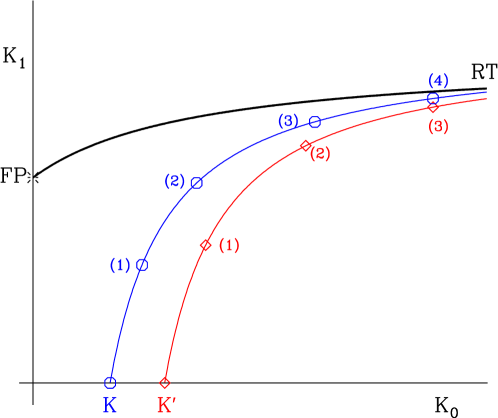
Figure 4: RG flow in bare parameter space. The points correspond to successive blocking steps. The figure is taken from Ref. [66].

To identify such a pair of couplings, we need to show that after $n$ and $(n-1)$ RG steps respectively their actions are identical. Explicitly calculating the actions would be complicated, but instead the gauge configurations themselves can be blocked; showing that the expectation values of all observables on these gauge configurations agree is equivalent to directly comparing the actions that generated them.

This procedure identifies, for each $n$, a pair of bare gauge couplings $(g,g^{\prime})$, or equivalently $(\beta,\beta^{\prime})$ where $\beta=2N/g^{2}$, with lattice correlation lengths that differ by a factor $s$, $\hat{\xi}^{\prime}=\hat{\xi}/s$. In the limit $n\rightarrow\infty$, it is customary to define the step scaling function for the bare coupling: $\Delta\beta=\beta-\beta^{\prime}\equiv s_{b}(\beta;s)$. This is the analogue of the Schrödinger Functional step scaling function for the renormalised coupling, $\sigma(u,s)$, and in the UV limit where $\overline{g}^{2}\rightarrow g_{0}^{2}=2N/\beta$, there is a simple relation between the two:

$$\frac{s_{b}(\beta;s)}{\beta}=\frac{\sigma(u,s)}{u}-1\,.$$ (28)

Clearly an IRFP is found when $s_{b}(\beta^{*};s)=0$, while $s_{b}$ is expected to remain positive for a QCD-like theory.

There is a degree of arbitrariness in choosing the blocking transformation, see e.g. Ref. [66]. Recent studies have used:

$$V_{n,\mu}=\mathrm{Proj}\left[(1-\alpha)U_{n,\mu}U_{n+\mu,\mu}+\frac{\alpha}{6}\sum_{\nu\neq\mu}U_{n,\nu}U_{n+\nu,\mu}U_{n+\mu+\nu,\mu}U_{n+2\mu,\nu}^{\dagger}\right]\,,$$ (29)

where $\alpha$ is a free parameter, which can be varied to optimise the transformation. Another possible choice for blocking is to perform a so-called HYP-smearing [67, 68]. Changing the blocking transformation changes the location of the fixed point, and the rate of convergence towards the RT. Ideally it should be chosen such that: (i) All observables yield the same $(g,g^{\prime})$ pairs for a given number of blocking steps $n$. Deviations are a measure of the systematic error from not being at exactly the same point along the RT; (ii) consecutive blocking steps predict the same matching coupling, i.e. for a given $g$, the matching coupling $g^{\prime}$ should be the same for all $n$. Deviations show that the irrelevant couplings still have sizeable effects. MCRG yields robust information only if these systematic errors are under control.

3 Results 2010

We shall summarize here the latest results at the time of the Lattice Conference. Previous studies have been summarized in the plenary talks at the Lattice Conferences in 2008 and 2009 [69, 70].

3.1 SU(3) with fundamental fermions

Starting from the upper end of the conformal window $n_{f}=16$, several theories have been studied with decreasing numbers of fermions.

At $n_{f}=16$ the two-loop beta function predicts an IRFP at weak coupling, $g_{0}^{2}\approx 0.5$. MCRG studies of this theory [67] have found a negative step scaling function $s_{b}$, in agreement with the hypothesis that the theory is indeed inside the conformal window. The bare step scaling function is shown to the left of Fig. 5. Different types of blocking yield different locations of the zero of the step scaling function, as expected since the position of the fixed point depends on the renormalization (or blocking) scheme.

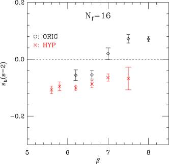
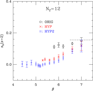
Figure 5: Bare step scaling function for $n_{f}=16$ (left) and $n_{f}=12$ (right) using the ORIG ($\diamond$), and the HYP ($\times$) blocking procedures; details about the blocking procedure can be found in Ref. [67].

At $n_{f}=12$ the situation is less clear. MCRG studies suggest a slow running of the coupling, but do not provide a clear cut answer about the existence of a fixed point. The bare step scaling is shown on the right of Fig. 4. The main limitation is the fact that these simulations require to run the code at exceedingly large values of the bare coupling [67]. Larger lattices could help to improve these results by allowing more blocking steps.

Studies of the running of the coupling defined through potential schemes do not show any sign of a conformal fixed point in this case. We refer the reader to the talks of Itou and Holland in these Proceedings [71, 72] for more details on these studies, which disagree with the results presented in Refs. [73, 74].

Spectral studies for this theory have not reached consensus yet. Some are consistent with the spectrum of a confining theory [75, 76, 56]. A summary of these results is reported in Fig. 6. However other studies fit well the hypothesis that the theory is in a chirally symmetric regime [77, 78, 79, 80]. As discussed in the previous section, there are a number of systematic errors that are likely to obscure the physically meaningful results, and more extensive simulations will be required to settle this issue.

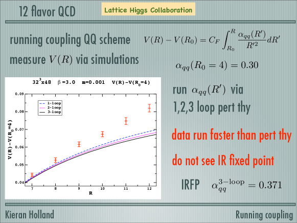
Figure 6: Spectrum studies for SU(3) with $n_{f}=12$. The upper plots show the pseudoscalar masses. The lower plots display, from left to right, the GMOR relation, the pion decay constant, and the chiral condensate. Lines correspond to fits to chiral perturbation theory [75].

As $n_{f}$ is further decreased, results for $n_{f}=10,9,8$ indicate these theories are already below the edge of the conformal window [67, 56].

Recent results, which appeared after the Lattice conference, suggest instead that the theory with $n_{f}=10$ lies inside the conformal window [81].

The LSD collaboration has been studying the $n_{f}=6$ theory. This theory is expected to be in the confining regime, sufficiently close to the edge of the conformal window to display a walking behaviour. An enhancement of the chiral condensate by a factor of 2 at the cutoff scale, and a possible trend towards parity doubling for the mesonic states have been identified [82]. The phenomenological implications of these findings need to be studied in more detail.

3.2 SU(2) with adjoint fermions

The SU(2) gauge theory with $n_{f}=2$ flavors in the adjoint representation has been investigated by several groups using different methods. In this case all simulations seem to indicate that the theory is inside the conformal window.

Recent studies are reported in Refs. [83, 28, 84, 85, 86, 87, 88, 50, 89]. Simulations so far have been performed with non-improved Wilson fermions; the phase diagram for the lattice theory has been mapped carefully in Refs. [87, 85], where a bulk phase transition was found and the region connected to continuum physics has been identified. Simulations have been performed trying to reach the small mass regime while preserving the hierarchy of scales required to control the systematic errors:

$$\left(\frac{L}{a}\right)\ll am_{\mathrm{PS}}\ll\left(\frac{r_{0}}{a}\right)^{-1}\ll 1\,,$$ (30)

where $L$ is the lattice size, $m_{\mathrm{PS}}$ is the lightest mass in the mesonic spectrum, and $r_{0}$ is the Sommer radius. Satisfying the above inequalities at small fermion masses becomes very rapidly a CPU-intensive task. New results for the spectrum were presented at this Conference [90, 91, 92]. Fig. 7 summarizes the most striking features observed in the spectrum, namely the near-degeneracy of the pseudoscalar and the vector meson mass, which persists at the smallest masses explored so far, and the large ratio of the pseudoscalar mass to the string tension. Both behaviours are at odds with the expected behaviour in a theory where chiral symmetry is spontaneously broken. In the latter case, the pseudoscalar mass goes to zero, while the other two quantities remain finite, thus yielding respectively a divergent and a vanishing ratio for the quantities in Fig. 7. Another interesting aspect of the spectrum study presented in Ref. [93] is the hierarchy between the glueball and the mesonic states, with the former being lighter than the latter. The mass of the glueballs scales with the fermion mass $m$, indicating that the system is not in the heavy mass regime. This result suggests that the light glueball states need to be included in any effective lagrangian description of TC low-energy dynamics. Note that these results have been obtained at a single value of the lattice spacing and therefore the size of lattice artefacts cannot be estimated properly.

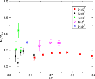
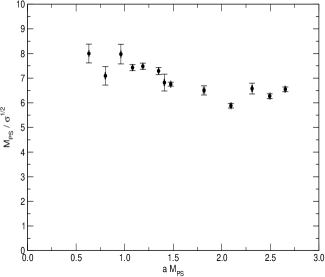
Figure 7: Vector meson to pseudoscalar meson mass ratio (left); notice that the two states remain degenerate when the mass is decreased. Ratio of the pseudoscalar mass to the square root of the string tension (right). The pseusoscalar mass and the string tension vanish at the same rate, yielding a finite ratio.

Finite size scaling can be tested by rescaling data obtained on lattices of varying size. Assuming the existence of an IRFP, data from different lattices should fall on a universal curve, e.g. for the pseudoscalar decay constant:

$$LF_{\mathrm{PS}}=\mathcal{F}(L^{y_{m}}m)\,.$$ (31)

Finite size scaling curves are displayed in Fig. 8, where different values of the scaling exponent $y_{m}=1+\gamma_{*}$ are used for rescaling the data. The plot indicates that the numerical results are consistent with the existence of an IRFP with a low value for $y_{m}$.

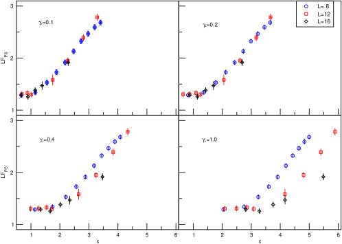
Figure 8: Finite size scaling curves for the pseudoscalar decay constant. The four plots, clockwise from the top left corner, correspond to scaling exponents $\gamma_{*}=0.1,0.2,0.5,0.4$ respectively.

Schrödinger functional studies for this theory show some evidence in favour of the existence of a conformal fixed point. The running of the gauge coupling was studied in Refs. [94, 27]. The results are summarized in Fig. 9. The plot on the left shows the continuum step scaling function, an IRFP is signalled by the condition $\sigma(u)/u=1$. The plot on the right is simply the difference of the renormalized couplings at scales $L_{1}$ and $L_{2}$; with the latter choice of variables the IRFP is identified by the difference of the two couplings, $\Delta(L_{1},L_{2})$, changing sign. Note that in this second way of presenting the data, the continuum limit is not taken, but the lattices with larger values of $L_{1}$ are closer to the continuum limit. In both cases, we see that the data are compatible with the existence of a fixed point. However the current error on the data (especially when performing the continuum extrapolation) is too large to locate precisely the critical value $g^{*}$. This is not surprising if the theory is really conformal, or near the edge of the conformal window. When the running of the coupling becomes very slow, the SF simulations have to resolve a very small signal that is easily obscured by the statistical and systematic errors. This is a common problem of all the studies of the running coupling for conformal theories.

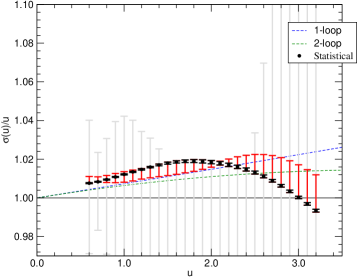
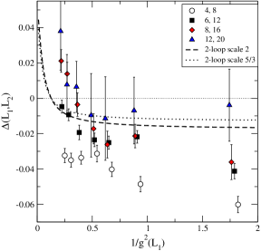
Figure 9: Running of the coupling constant in the SF scheme. Data are taken from Ref. [27] for the left plot, and Ref. [94] for the right one. The large error bands in the plot on the left are due to the continuum extrapolation of the step scaling function.

Finally, as discussed in the previous Section, the SF can be used to study the running of the mass and therefore deduce the anomalous dimension $\gamma$ [27]. Data for $\sigma_{P}(u)$ are displayed in Fig. 10.

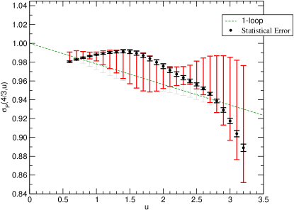
Figure 10: Running of the mass computed from the SF [27].

Note that the step scaling function $\sigma_{P}$ is not small for a conformal theory, and therefore can be measured with better accuracy. Interestingly its value does not display any statistically significant deviation from the one-loop prediction.

The anomalous dimension $\gamma_{*}$ can be read from the curve in Fig. 10, as long as the value of the gauge coupling at the fixed point is precisely known. Unfortunately, as discussed above, the latter cannot be located precisely; the uncertainty on the value of $g^{*}$ is the main source of uncertainty in the determination of the mass anomalous dimension. With the current data the best estimate is:

$$0.05<\gamma_{*}<0.56\,.$$ (32)

Preliminary results using the MCRG technique seem to confirm this estimate [95].

Recent results confirming the picture above have recently appeared [96].

Results obtained with different techniques are consistent with the existence of an IRFP for these theory, with a small value of the anomalous dimension. The phenomenological consequences of such a small value need to be investigated carefully.

3.3 SU(3) with sextet fermions

Results have also been obtained for the SU(3) gauge theory with $n_{f}=2$ in the two-index symmetric representation, i.e. the sextet representation of SU(3). This model has also been proposed for phenomenological applications under the name of Next to Minimal Walking Technicolor (NMWT).

Results for the spectrum and the eigenvalues of the Dirac operator have been presented in Refs. [97, 98, 99, 100, 101, 102, 44].

Results for the SF lattice step scaling function $\Sigma(u)$ have been presented at this Conference [103], showing evidence of a slow running of the coupling. Different discretizations yield statistically inconsistent estimates for the location of the fixed point coupling $g^{*}$, emphasizing the importance of controlling the size of lattice artefacts in these studies. The difference

$$B(u,2)=-1/g^{2}(L)+1/g^{2}(2L)$$ (33)

is displayed on the left-hand side in Fig. 11, computed using thin links ($\diamond$) and fat links ($\square$) respectively. The difference between the diamond curve and the square curve shows the effect of lattice artefacts.

Once again, results for the mass anomalous dimension have a much smaller relative error, as seen in the plot on the right of Fig. 11. The estimates obtained from the SF, from finite size scaling, and from the eigenvalues of the Dirac operator are in broad agreement, and suggest the bound $\gamma_{*}<0.6$.

Studies at finite temperature on the other hand indicate that the theory is outside the conformal window and “slow walking” [104, 105].

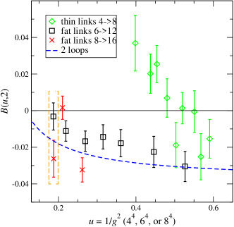
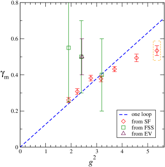
Figure 11: Running of the coupling (left) and the mass (right) for the SU(3) theory with two flavors in the two-index symmetric representation [103].

A detailed computation of the spectrum has been performed with staggered fermions for the same theory, and presented at this Conference [75]. The numerical data in this case are consistent with chiral symmetry breaking.

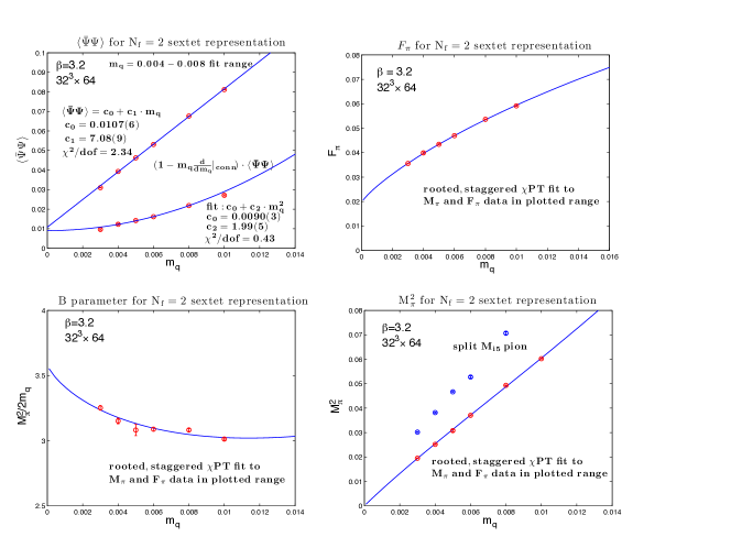
Figure 12: Chiral extrapolation of the chiral condensate and other spectral quantities. Data are consistent with rooted staggered chiral perturbation theory [75].

Further work is needed to reach consensus on the long-distance dynamics in this case.

4 Outlook

There have been numerous studies of nonperturbative dynamics beyond QCD in the last two years. Several theories that are expected to be at the edge of the conformal window have been investigated, using the tools described in Section 2. This is an interesting problem in field theory, and there are several intriguing data, suggesting that first evidence for the existence of fixed points has been found. However robust results can be obtained only by keeping the systematic errors under control.

In particular simulations must be performed at small masses, on large volumes, trying to minimize lattice artefacts that can obscure the physically interesting features. Preliminary results about simulations with improved actions for the SU(2) theory have been presented in Refs. [106, 107]. At the same time it is worthwhile to keep looking for better observables that can yield unambiguous signals.

It is important to develop a strong link with the phenomenological work and the data analyses at the LHC. Lattice data will have an impact on phenomenology only if the relevant questions are identified and answered in a quantitative way. A wishlist of interesting issues has been discussed by Chivukula at this Conference [108].

- [1] Kenneth A. Intriligator and N. Seiberg. Lectures on supersymmetric gauge theories and electric- magnetic duality. Nucl. Phys. Proc. Suppl., 45BC:1–28, 1996.
- [2] Francesco Sannino. Conformal Dynamics for TeV Physics and Cosmology. 2009.
- [3] Erich Poppitz and Mithat Unsal. Conformality or confinement: (IR)relevance of topological excitations. JHEP, 09:050, 2009.
- [4] Carlos Nunez, Ioannis Papadimitriou, and Maurizio Piai. Walking Dynamics from String Duals. 2008.
- [5] Adi Armoni. The Conformal Window from the Worldline Formalism. Nucl. Phys., B826:328–336, 2010.
- [6] K. Nakamura. Review of particle physics. J. Phys., G37:075021, 2010.
- [7] Steven Weinberg. Implications of Dynamical Symmetry Breaking. Phys. Rev., D13:974–996, 1976.
- [8] Leonard Susskind. Dynamics of Spontaneous Symmetry Breaking in the Weinberg- Salam Theory. Phys. Rev., D20:2619–2625, 1979.
- [9] Estia Eichten and Kenneth D. Lane. Dynamical breaking of weak interaction symmetries. Phys. Lett., B90:125–130, 1980.
- [10] Savas Dimopoulos and Leonard Susskind. Mass Without Scalars. Nucl. Phys., B155:237–252, 1979.
- [11] Thomas Appelquist, Maurizio Piai, and Robert Shrock. Fermion masses and mixing in extended technicolor models. Phys. Rev., D69:015002, 2004.
- [12] Roberto Contino. Tasi 2009 lectures: The Higgs as a Composite Nambu- Goldstone Boson. 2010.
- [13] Christopher T. Hill and Elizabeth H. Simmons. Strong dynamics and electroweak symmetry breaking. Phys. Rept., 381:235–402, 2003.
- [14] Bob Holdom. Raising the sideways scale. Phys. Rev., D24:1441, 1981.
- [15] Bob Holdom. Techniodor. Phys. Lett., B150:301, 1985.
- [16] Koichi Yamawaki, Masako Bando, and Ken-iti Matumoto. Scale invariant technicolor model and a technidilaton. Phys. Rev. Lett., 56:1335, 1986.
- [17] T. Akiba and T. Yanagida. Hierarchic Chiral Condensate. Phys. Lett., B169:432, 1986.
- [18] Thomas W. Appelquist, Dimitra Karabali, and L. C. R. Wijewardhana. Chiral Hierarchies and the Flavor Changing Neutral Current Problem in Technicolor. Phys. Rev. Lett., 57:957, 1986.
- [19] Thomas Appelquist and L. C. R. Wijewardhana. Chiral Hierarchies from Slowly Running Couplings in Technicolor Theories. Phys. Rev., D36:568, 1987.
- [20] Thomas Appelquist and Francesco Sannino. The physical spectrum of conformal SU(N) gauge theories. Phys. Rev., D59:067702, 1999.
- [21] R. Sekhar Chivukula and Elizabeth H. Simmons. Condensate Enhancement and D-Meson Mixing in Technicolor Theories. Phys. Rev., D82:033014, 2010.
- [22] G. Mack. All Unitary Ray Representations of the Conformal Group SU(2,2) with Positive Energy. Commun. Math. Phys., 55:1, 1977.
- [23] Michael Edward Peskin and Tatsu Takeuchi. A New constraint on a strongly interacting Higgs sector. Phys. Rev. Lett., 65:964–967, 1990.
- [24] Guido Altarelli and Riccardo Barbieri. Vacuum polarization effects of new physics on electroweak processes. Phys. Lett., B253:161–167, 1991.
- [25] Witold Skiba. TASI Lectures on Effective Field Theory and Precision Electroweak Measurements. 2010.
- [26] Maurizio Piai. Lectures on walking technicolor, holography and gauge/gravity dualities. 2010.
- [27] Francis Bursa, Luigi Del Debbio, Liam Keegan, Claudio Pica, and Thomas Pickup. Mass anomalous dimension in SU(2) with two adjoint fermions. Phys. Rev., D81:014505, 2010.
- [28] Luigi Del Debbio, Mads T. Frandsen, Haralambos Panagopoulos, and Francesco Sannino. Higher representations on the lattice: perturbative studies. JHEP, 06:007, 2008.
- [29] William E. Caswell. Asymptotic Behavior of Nonabelian Gauge Theories to Two Loop Order. Phys. Rev. Lett., 33:244, 1974.
- [30] Tom Banks and A. Zaks. On the phase structure of vector-like gauge theories with massless fermions. Nucl. Phys., B196:189, 1982.
- [31] Dennis D. Dietrich and Francesco Sannino. Conformal window of su(n) gauge theories with fermions in higher dimensional representations. Phys. Rev., D75:085018, 2007.
- [32] Markus A. Luty and Takemichi Okui. Conformal technicolor. JHEP, 09:070, 2006.
- [33] Dennis D. Dietrich, Francesco Sannino, and Kimmo Tuominen. Light composite Higgs from higher representations versus electroweak precision measurements: Predictions for LHC. Phys. Rev., D72:055001, 2005.
- [34] Hidenori S. Fukano and Francesco Sannino. Conformal Window of Gauge Theories with Four-Fermion Interactions and Ideal Walking. 2010.
- [35] Andrew G. Cohen and Howard Georgi. WALKING BEYOND THE RAINBOW. Nucl. Phys., B314:7, 1989.
- [36] Thomas Appelquist, John Terning, and L. C. R. Wijewardhana. The Zero Temperature Chiral Phase Transition in SU(N) Gauge Theories. Phys. Rev. Lett., 77:1214–1217, 1996.
- [37] Thomas Appelquist, Anuradha Ratnaweera, John Terning, and L. C. R. Wijewardhana. The phase structure of an SU(N) gauge theory with N(f) flavors. Phys. Rev., D58:105017, 1998.
- [38] Einan Gardi and Georges Grunberg. The conformal window in QCD and supersymmetric QCD. JHEP, 03:024, 1999.
- [39] Thomas A. Ryttov and Francesco Sannino. Supersymmetry Inspired QCD Beta Function. Phys. Rev., D78:065001, 2008.
- [40] Riccardo Rattazzi, Vyacheslav S. Rychkov, Erik Tonni, and Alessandro Vichi. Bounding scalar operator dimensions in 4D CFT. JHEP, 12:031, 2008.
- [41] Rajamani Narayanan and Herbert Neuberger. A survey of large N continuum phase transitions. PoS, LAT2007:020, 2007.
- [42] Guido Cossu and Massimo D’Elia. Finite size phase transitions in QCD with adjoint fermions. JHEP, 07:048, 2009.
- [43] Thomas DeGrand and Anna Hasenfratz. Remarks on lattice gauge theories with infrared-attractive fixed points. Phys. Rev., D80:034506, 2009.
- [44] Thomas DeGrand. Finite-size scaling tests for SU(3) lattice gauge theory with color sextet fermions. Phys. Rev., D80:114507, 2009.
- [45] Luigi Del Debbio, Biagio Lucini, Agostino Patella, Claudio Pica, and Antonio Rago. Mesonic spectroscopy of Minimal Walking Technicolor. 2010.
- [46] Luigi Del Debbio and Roman Zwicky. Hyperscaling relations in mass-deformed conformal gauge theories. Phys. Rev., D82:014502, 2010.
- [47] Luigi Del Debbio and Roman Zwicky. Scaling relations for the entire spectrum in mass-deformed conformal gauge theories. 2010.
- [48] Markus A. Luty. Strong Conformal Dynamics at the LHC and on the Lattice. JHEP, 04:050, 2009.
- [49] Francesco Sannino. Conformal Chiral Dynamics. Phys. Rev., D80:017901, 2009.
- [50] L. Del Debbio, B. Lucini, A. Patella, C. Pica, and A. Rago. Conformal vs confining scenario in SU(2) with adjoint fermions. Phys. Rev., D80:074507, 2009.
- [51] L. Del Debbio, S.J. Hands, and J.C. Mehegan. The Three-dimensional Thirring model for small N(f). Nucl.Phys., B502:269–308, 1997.
- [52] Jens Braun and Holger Gies. Scaling laws near the conformal window of many-flavor QCD. 2009.
- [53] Jens Braun, Christian S. Fischer, and Holger Gies. Beyond Miransky Scaling. 2010. * Temporary entry *.
- [54] V. A. Miransky. Dynamics in the conformal window in QCD like theories. Phys. Rev., D59:105003, 1999.
- [55] H. Leutwyler. ENERGY LEVELS OF LIGHT QUARKS CONFINED TO A BOX. Phys. Lett., B189:197, 1987.
- [56] Zoltan Fodor, Kieran Holland, Julius Kuti, Daniel Nogradi, and Chris Schroeder. Nearly conformal gauge theories in finite volume. Phys. Lett., B681:353–361, 2009.
- [57] Martin Luscher, Peter Weisz, and Ulli Wolff. A numerical method to compute the running coupling in asymptotically free theories. Nucl. Phys., B359:221–243, 1991.
- [58] Martin Luscher, Rajamani Narayanan, Peter Weisz, and Ulli Wolff. The Schrodinger functional: A Renormalizable probe for nonAbelian gauge theories. Nucl. Phys., B384:168–228, 1992.
- [59] Stefano Capitani, Martin Luscher, Rainer Sommer, and Hartmut Wittig. Non-perturbative quark mass renormalization in quenched lattice qcd. Nucl. Phys., B544:669–698, 1999.
- [60] Michele Della Morte et al. Non-perturbative quark mass renormalization in two-flavor QCD. Nucl. Phys., B729:117–134, 2005.
- [61] Erek Bilgici et al. A new scheme for the running coupling constant in gauge theories using Wilson loops. Phys. Rev., D80:034507, 2009.
- [62] Zoltan Fodor, Kieran Holland, Julius Kuti, Daniel Nogradi, and Chris Schroeder. Calculating the running coupling in strong electroweak models. 2009.
- [63] A. Hasenfratz, P. Hasenfratz, Urs M. Heller, and F. Karsch. IMPROVED MONTE CARLO RENORMALIZATION GROUP METHODS. Phys. Lett., B140:76, 1984.
- [64] A. Hasenfratz, P. Hasenfratz, Urs M. Heller, and F. Karsch. THE beta FUNCTION OF THE SU(3) WILSON ACTION. Phys. Lett., B143:193, 1984.
- [65] K. C. Bowler et al. Monte carlo renormalization group studies of su(3) lattice gauge theory. Nucl. Phys., B257:155–172, 1985.
- [66] Anna Hasenfratz. Investigating the critical properties of beyond-QCD theories using Monte Carlo Renormalization Group matching. Phys. Rev., D80:034505, 2009.
- [67] Anna Hasenfratz. Conformal or Walking? Monte Carlo renormalization group studies of SU(3) gauge models with fundamental fermions. Phys. Rev., D82:014506, 2010.
- [68] Anna Hasenfratz and Francesco Knechtli. Flavor symmetry and the static potential with hypercubic blocking. Phys. Rev., D64:034504, 2001.
- [69] George T. Fleming. Strong Interactions for the LHC. PoS, LATTICE2008:021, 2008.
- [70] Elisabetta Pallante. Strongly and slightly flavored gauge theories. 2009.
- [71] E. Itou. Search for IR fixed point in the Twisted Polyakov Loop scheme (II). PoS, LATTICE2010:054, 2010.
- [72] K. Holland. Running couplings in 12 flavors QCD. PoS, LATTICE2010:053, 2010.
- [73] Thomas Appelquist, George T. Fleming, and Ethan T. Neil. Lattice Study of the Conformal Window in QCD-like Theories. Phys. Rev. Lett., 100:171607, 2008.
- [74] Thomas Appelquist, George T. Fleming, and Ethan T. Neil. Lattice Study of Conformal Behavior in SU(3) Yang-Mills Theories. Phys. Rev., D79:076010, 2009.
- [75] J. Kuti. Toward the nearly conformal composite Higgs mechanism. PoS, LATTICE2010:060, 2010.
- [76] X.Y. Jin. Lattice QCD with 8 and 12 degenerate quark flavors. PoS, LATTICE2010:055, 2010.
- [77] M.P. Lombardo. Chiral symmetry of QCD with 12 light flavors. PoS, LATTICE2010:062, 2010.
- [78] E. Pallante. The bulk transition of many-flavor QCD and the search for an UVFP at strong coupling. PoS, LATTICE2010:067, 2010.
- [79] A. Deuzeman, M. P. Lombardo, and E. Pallante. Evidence for a conformal phase in SU(N) gauge theories. Phys. Rev., D82:074503, 2010.
- [80] Albert Deuzeman, Maria Paola Lombardo, and Elisabetta Pallante. Traces of a fixed point: Unravelling the phase diagram at large Nf. 2009.
- [81] M. Hayakawa, K.-I. Ishikawa, Y. Osaki, S. Takeda, S. Uno, et al. Running coupling constant of ten-flavor QCD with the Schródinger functional method. 2010. * Temporary entry *.
- [82] G.T. Fleming. SU(3) lattice gauge theory for two, six, and ten flavors. PoS, LATTICE2010:049, 2010.
- [83] Simon Catterall and Francesco Sannino. Minimal walking on the lattice. Phys. Rev., D76:034504, 2007.
- [84] Luigi Del Debbio, Agostino Patella, and Claudio Pica. Higher representations on the lattice: numerical simulations. SU(2) with adjoint fermions. 2008.
- [85] Simon Catterall, Joel Giedt, Francesco Sannino, and Joe Schneible. Phase diagram of SU(2) with 2 flavors of dynamical adjoint quarks. JHEP, 11:009, 2008.
- [86] Luigi Del Debbio, Agostino Patella, and Claudio Pica. Fermions in higher representations. Some results about SU(2) with adjoint fermions. 2008.
- [87] Ari J. Hietanen, Jarno Rantaharju, Kari Rummukainen, and Kimmo Tuominen. Spectrum of SU(2) lattice gauge theory with two adjoint Dirac flavours. JHEP, 05:025, 2009.
- [88] Ari Hietanen, Jarno Rantaharju, Kari Rummukainen, and Kimmo Tuominen. Spectrum of SU(2) gauge theory with two fermions in the adjoint representation. PoS, LATTICE2008:065, 2008.
- [89] C. Pica, L. Del Debbio, B. Lucini, A. Patella, and A. Rago. Technicolor on the Lattice. 2009.
- [90] C. Pica. Confining vs. conformal scenario for SU(2) with 2 adjoint fermions. Mesonic spectrum. PoS, LATTICE2010:069, 2010.
- [91] A. Patella. Confining vs. conformal scenario for SU(2) with adjoint fermions. Gluonic observables. PoS, LATTICE2010:068, 2010.
- [92] E. Kerrane. Improved Lattice Spectroscopy of Minimal Walking Technicolor. PoS, LATTICE2010:058, 2010.
- [93] Luigi Del Debbio, Biagio Lucini, Agostino Patella, Claudio Pica, and Antonio Rago. The infrared dynamics of Minimal Walking Technicolor. 2010.
- [94] Ari J. Hietanen, Kari Rummukainen, and Kimmo Tuominen. Evolution of the coupling constant in SU(2) lattice gauge theory with two adjoint fermions. Phys. Rev., D80:094504, 2009.
- [95] L. Keegan. MCRG Minimal Walking Technicolor. PoS, LATTICE2010:057, 2010.
- [96] Thomas DeGrand, Yigal Shamir, and Benjamin Svetitsky. Infrared fixed point in SU(2) gauge theory with adjoint fermions. 2011. * Temporary entry *.
- [97] Thomas DeGrand, Yigal Shamir, and Benjamin Svetitsky. Exploring the phase diagram of sextet QCD. PoS, LATTICE2008:063, 2008.
- [98] Thomas DeGrand, Yigal Shamir, and Benjamin Svetitsky. Phase structure of SU(3) gauge theory with two flavors of symmetric-representation fermions. Phys. Rev., D79:034501, 2009.
- [99] Zoltan Fodor, Kieran Holland, Julius Kuti, Daniel Nogradi, and Chris Schroeder. Nearly conformal electroweak sector with chiral fermions. PoS, LATTICE2008:058, 2008.
- [100] Zoltan Fodor, Kieran Holland, Julius Kuti, Daniel Nogradi, and Chris Schroeder. Chiral properties of SU(3) sextet fermions. JHEP, 11:103, 2009.
- [101] Zoltan Fodor, Kieran Holland, Julius Kuti, Daniel Nogradi, and Chris Schroeder. Topology and higher dimensional representations. JHEP, 08:084, 2009.
- [102] Thomas DeGrand. Volume scaling of Dirac eigenvalues in SU(3) lattice gauge theory with color sextet fermions. 2009.
- [103] Y. Shamir B. Svetitsky and T. DeGrand. Sextet QCD: slow running and the mass anomalous dimension. PoS, LATTICE2010:072, 2010.
- [104] J. B. Kogut and D. K. Sinclair. Thermodynamics of lattice QCD with 2 flavours of colour- sextet quarks: A model of walking/conformal Technicolor. Phys. Rev., D81:114507, 2010.
- [105] D.K. Sinclair. New results with colour-sextet quarks. PoS, LATTICE2010:071, 2010.
- [106] Tuomas Karavirta, Anne-Mari Mykkanen, Jarno Rantaharju, Kari Rummukainen, and Kimmo Tuominen. Perturbative improvement of SU(2) gauge theory with two Wilson fermions in the adjoint representation. PoS, LATTICE2010:056, 2010.
- [107] Anne Mykkanen, Jarno Rantaharju, Kari Rummukainen, Tuomas Karavirta, and Kimmo Tuominen. Non-perturbatively improved clover action for SU(2) gauge + fundamental and adjoint representation fermions. PoS, LATTICE2010:064, 2010.
- [108] R. Sekhar Chivukula and Elizabeth H. Simmons. Technicolor and Lattice Gauge Theory. PoS, LATTICE2010:003, 2010.