Analytical spectral-domain scattering theory of a general gyrotropic sphere

Abstract

We propose an analytical scattering theory in spectral domain to model the electromagnetic (EM) fields of a gyrotropic sphere in terms of the eigen-functions and their associated spectral eigenvalues/coefficients in a recursive integral form. Applying the continuous boundary conditions of electromagnetic fields on the surface between the free space and gyrotropic sphere, the spectral coefficients of transmitted fields inside the gyrotropic sphere and the scattered fields in the isotropic host medium can be obtained exactly by expanding spherical vector wave eigenfunctions. Numerical results are provided for some representative cases, which are compared to the results from adaptive integral method (AIM). Good agreement demonstrates the validity of the proposed analytical scattering theory for gyrotropic spheres in spectral domain using Fourier transform.

I Introduction

Electromagnetic scattering of anisotropic media have attracted more and more attention for their wide applications in the past decades, such as radar cross section (RCS) computation of perfect electric conductor (PEC) targets coated with complex material, radome design, and interaction of light/wave with biological media and metamaterials ref1 ; ref2 ; ref3 ; ref6 ; ref7 ; ref8 ; ref9 ; ref9a ; ref9b ; ref11 ; ref12 .

Based on the plane wave expansion in terms of spherical vector wave functions in isotropic medium ref13 , the scattering by a uniaxial sphere and a sphere of uniaxial left-handed materials have been derived ref11 ; ref12 . More recently, the scattering of a gyromagnetic sphere has been investigated in the expansion in spatial domain ref12b . Moreover, the theory is only working for the case having gyrotropic permeability and scalar permittivity. If both permittivity and permeability are gyrotropic matrices, the interplay between the extra three parameters in the gyrotropic permittivity will make that approach ref12b too tedious and insufficient to model the scattering properties. This motivates our work in spectral domain instead of spatial domain. A most general gyrotropic sphere is considered, and since the existing method has drawbacks in the analysis of scatterings, a novel approach has to be developed. The analytical method, which can be readily implemented by programming, has its academic and practical significance in contrast to purely numerical solutions from FDTD, FEM or others.

In view of this, we propose a distinguished method based on Fourier transform, and thus the spectral-domain analysis of the scattering by a general gyrotropic sphere in terms of spherical functions wave functions is investigated. This method has distinguished features: (1) it can straightforwardly be employed to describe the light wave interaction with particles and objects with gyrotropic permittivity and permeability; (2) the material constitution is very complex and general (both $\overline{\epsilon}$ and $\overline{\mu}$ are gyrotropic tensors), so all those existing scattering theorems are just its sub-cases, e.g., uniaxial, plasma, anisotropic, gyromagnetic, etc.; (3) it directly solves for the eigen-problems in spectral domain by Fourier transform, which simplifies the formulation in spatial domain ref12b .

To obtain the solution of vector wave functions in gyrotropic anisotropic media, we start from the vector wave equation in a source-free gyrotropic anisotropic medium. Taking the Fourier transform of the electric field and substituting it into the vector wave equation of the electric field, we obtain the characteristic equation. Solving this equation, the eigenvalues and corresponding vector wave eigenfunctions can be yielded. Then, electromagnetic fields inside and outside the gyrotropic anisotropic sphere can be expressed based on the eigenvalues and eigenfunctions. Those unknown scattering coefficients can be analytically determined from applying the continuous boundary conditions on the surface of the gyrotropic anisotropic sphere, where orthogonality relations of the Legendre polynomials are employed. Numerical results are obtained to gain more physical insight into this problem. After the results were validated by comparison with the existing data, some new results are computed and discussed.

In the subsequent analysis, a time dependence of the form exp$(-i\omega t)$ is assumed for the electromagnetic field quantities but is suppressed throughout the treatment.

II Analytical formulation

The permittivity and permeability tensors of the gyrotropic anisotropic sphere shown in Fig. 1 are characterized by the following two matrices

$$\overline{\epsilon} = \left[\begin{array}[]{ccc}\epsilon_{1}&-i\epsilon_{2}&0\\ i\epsilon_{2}&\epsilon_{1}&0\\ 0&0&\epsilon_{3}\end{array}\right]$$ (4)

$$\overline{\mu} = \left[\begin{array}[]{ccc}\mu_{1}&-i\mu_{2}&0\\ i\mu_{2}&\mu_{1}&0\\ 0&0&\mu_{3}\end{array}\right].$$ (8)

Figure 1: Geometry for the EM scattering of a plane wave by an gyrotropic anisotropic sphere.

The parameters are defined in Cartesian coordinates. The $E$-field vector wave equation can be obtained by substituting the above constitutive relations into the source-free Maxwell’s equations ref12 , i.e.,

$$\mbox{\boldmath$\nabla$}\times\left[\mbox{\boldmath$\overline{\mu}$}^{-1}\cdot\mbox{\boldmath$\nabla$}\times\mbox{\boldmath$E$}(\mbox{\boldmath$r$})\right]-\omega^{2}\mbox{\boldmath$\overline{\epsilon}$}\cdot\mbox{\boldmath$E$}(\mbox{\boldmath$r$})=0.$$ (9)

The solution to (9) can be obtained by the following Fourier transform:

$$\mbox{\boldmath$E$}(\mbox{\boldmath$r$})=\int^{\infty}_{-\infty}dk_{x}\int^{\infty}_{-\infty}dk_{y}\int^{\infty}_{-\infty}\mbox{\boldmath$E$}(\mbox{\boldmath$k$})e^{i\mbox{\boldmath$k$}\cdot\mbox{\boldmath$r$}}dk_{z}$$ (10)

where the wave number is denoted by $\mbox{\boldmath$k$}=k_{x}\mbox{$\widehat{\mbox{\boldmath$x$}}$}+k_{y}\mbox{$\widehat{\mbox{\boldmath$y$}}$}+k_{z}\mbox{$\widehat{\mbox{\boldmath$z$}}$}$, and the space vector is identified as $\mbox{\boldmath$r$}=x\mbox{$\widehat{\mbox{\boldmath$x$}}$}+y\mbox{$\widehat{\mbox{\boldmath$y$}}$}+z\mbox{$\widehat{\mbox{\boldmath$z$}}$}$, with $\widehat{\mbox{\boldmath$x$}}$, $\widehat{\mbox{\boldmath$y$}}$, $\widehat{\mbox{\boldmath$z$}}$ being the unit vectors in Cartesian coordinates. By substituting (3) into (2), the wave equation can be transformed into

$$\int^{\infty}_{-\infty}dk_{x}\int^{\infty}_{-\infty}dk_{y}\int^{\infty}_{-\infty}\mbox{\boldmath$\overline{K}$}(\mbox{\boldmath$k$})\cdot\mbox{\boldmath$E$}(\mbox{\boldmath$k$})e^{i\mbox{\boldmath$k$}\cdot\mbox{\boldmath$r$}}dk_{z}=0$$ (11)

where

$$\mbox{\boldmath$\overline{K}$}(\mbox{\boldmath$k$})=\\ \left[\begin{array}[]{ccc}-b_{1}k_{z}^{2}-b_{3}k^{2}_{y}+a_{1}&b_{3}k_{x}k_{y}-ib_{2}k^{2}_{z}-ia_{2}&b_{1}k_{x}k_{z}+ib_{2}k_{y}k_{z}\\ b_{3}k_{x}k_{y}+ib_{2}k^{2}_{z}+ia_{2}&-b_{1}k_{z}^{2}-b_{3}k^{2}_{x}+a_{1}&b_{1}k_{y}k_{z}-ib_{2}k_{x}k_{z}\\ b_{1}k_{x}k_{z}-ib_{2}k_{y}k_{z}&b_{1}k_{y}k_{z}+ib_{2}k_{x}k_{z}&-b_{1}(k_{y}^{2}+k^{2}_{x})+a_{3}\end{array}\!\!\right]$$ (12)

with

$$a_{1} = \omega^{2}\epsilon_{1},$$

$$a_{2} = \omega^{2}\epsilon_{2},$$

$$a_{3} = \omega^{2}\epsilon_{3},$$

$$b_{1} = \displaystyle\frac{\mu_{1}}{\mu^{2}_{1}-\mu^{2}_{2}}$$

$$b_{2} = \displaystyle\frac{\mu_{2}}{\mu^{2}_{1}-\mu^{2}_{2}}$$

$$b_{3} = 1/\mu_{3}.$$ (13)

In order to get nontrivial solutions of $\mbox{\boldmath$E$}(\mbox{\boldmath$k$})$, the following characteristic equation has to be satisfied:

$$\mbox{Det}\left[\mbox{\boldmath$\overline{K}$}(\mbox{\boldmath$k$})\right]=0.$$ (14)

It can be explicitly rewritten as

$$A(\theta_{k},\phi_{k})k^{4}-B(\theta_{k},\phi_{k})k^{2}+C=0,$$ (15)

where

$$A(\theta_{k},\phi_{k}) = \left[b_{1}b_{3}\sin^{2}\theta_{k}+(b^{2}_{1}-b^{2}_{2})cos^{2}\theta_{k}\right]\times\left[a_{1}\sin^{2}\theta_{k}+a_{3}\cos^{2}\theta_{k}\right],$$

$$B(\theta_{k},\phi_{k}) = \left[b_{1}(a^{2}_{1}-a^{2}_{2})+b_{3}a_{1}a_{3}\right]\sin^{2}\theta_{k}+2a_{3}(b_{1}a_{1}+b_{2}a_{2})\cos^{2}\theta_{k}$$

$$C = a_{3}(a^{2}_{1}-a^{2}_{2})$$ (16)

with

$$k^{2} = k^{2}_{x}+k^{2}_{y}+k^{2}_{z},$$

$$\theta_{k} = \tan^{-1}(\sqrt{k^{2}_{x}+k^{2}_{y}}/k_{z}),$$

$$\phi_{k} = \tan^{-1}(k_{y}/k_{x}).$$ (17)

Equation (15) is a biquadratic equation with the following four roots of $k_{\ell}$ (where $\ell=1,2,3$, or 4) for the radial wave vectors:

$$k^{2}_{1,3} = \frac{B+\sqrt{B^{2}-4AC}}{2A},$$

$$k^{2}_{2,4} = \frac{B-\sqrt{B^{2}-4AC}}{2A}.$$ (18)

So the corresponding $E$-field eigenvectors can be obtained from Eq. (12) and are given as follows

$$\mbox{\boldmath$E$}_{q} = \mbox{\boldmath$F$}^{e}_{q}f_{q}(\theta_{k},\phi_{k})=\bigg{[}F^{e}_{qx}(\theta_{k},\phi_{k})\mbox{$\widehat{\mbox{\boldmath$x$}}$}+F^{e}_{qy}(\theta_{k},\phi_{k})\mbox{$\widehat{\mbox{\boldmath$y$}}$}+F^{e}_{qz}(\theta_{k},\phi_{k})\mbox{$\widehat{\mbox{\boldmath$z$}}$}\bigg{]}f_{q}(\theta_{k},\phi_{k}),$$ (19)

where and subsequently, $q=1,2,3$, or 4; and

$$F_{qx}^{e} = -\displaystyle\frac{\triangle_{1}}{\triangle}sin\phi_{k}+\displaystyle\frac{\triangle_{2}}{\triangle}cos\phi_{k},$$

$$F_{qy}^{e} = \displaystyle\frac{\triangle_{1}}{\triangle}cos\phi_{k}+\frac{\triangle_{2}}{\triangle}sin\phi_{k},$$

$$F_{qz}^{e} = 1$$ (20)

with

$$\triangle_{1} = i(b_{1}a_{2}+b_{2}a_{1})k^{2}_{q}sin\theta_{k}cos\theta_{k}$$

$$\triangle_{2} = \left[b_{1}b_{3}k^{2}_{q}sin^{2}\theta_{k}+(b^{2}_{1}-b^{2}_{2})k^{2}_{q}cos^{2}\theta_{k}\right]k^{2}_{q}sin\theta_{k}cos\theta_{k}-(b_{1}a_{1}+b_{2}a_{2})$$

$$\triangle = -(b_{2}k^{2}_{q}cos^{2}\theta_{k}+a_{2})^{2}+(b_{1}k^{2}_{q}cos^{2}\theta_{k}-a_{1})(b_{1}k^{2}_{q}cos^{2}\theta_{k}+b_{3}k^{2}_{q}sin^{2}\theta_{k}-a_{1})$$ (21)

With those obtained eigenvalues and their associated formulas, the $E$-field in Eq. (10) is then given as follows

$$\mbox{\boldmath$E$}(\mbox{\boldmath$r$}) = \sum^{2}_{q=1}\int^{\pi}_{0}\int^{2\pi}_{0}\mbox{\boldmath$F$}^{e}_{q}(\theta_{k},\phi_{k})f_{q}(\theta_{k},\phi_{k})e^{i\mbox{\boldmath$k$}_{q}\cdot\mbox{\boldmath$r$}}k^{2}_{q}\sin\theta_{k}d\theta_{k}d\phi_{k}$$ (22)

where

$$\mbox{\boldmath$k$}_{q}=k_{q}\sin\theta_{k}\cos\phi_{k}\mbox{$\widehat{\mbox{\boldmath$x$}}$}+k_{q}\sin\theta_{k}\sin\phi_{k}\mbox{$\widehat{\mbox{\boldmath$y$}}$}+k_{q}\cos\theta_{k}\mbox{$\widehat{\mbox{\boldmath$z$}}$},$$

and $f_{q}(\theta_{k},\phi_{k})$ denotes the unknown angular spectrum amplitude. Equation (22) is also known as the eigen plane wave spectrum representation of the electric field in homogeneous gyrotropic anisotropic medium. From (10), it is evident that the integration over the radial wave-vector component is reduced to a summation of four terms corresponding to the roots of (15), which are the only permissible solutions. The symmetric roots, i.e., $k=-k_{q}$ of $k=k_{q}$ $(q=1,2)$ are taken into account automatically as $\theta$ spans from 0 to $\pi$ while $\phi$ spans from 0 to $2\pi$. Physically, we need to sum up for only two of the four components, namely, $k_{1}$ and $k_{2}$.

It is noted that the unknown angular spectrum amplitude $f_{q}(\theta_{k},\phi_{k})$ is a periodic function with respect to $\theta_{k}$ and $\phi_{k}$. Therefore we can use surface harmonics of the first kind to expand the $f_{q}(\theta_{k},\phi_{k})$

$$f_{q}(\theta_{k},\phi_{k})=\sum_{m^{\prime},n^{\prime}}G_{m^{\prime}n^{\prime}q}P^{m^{\prime}}_{n^{\prime}}(\cos\theta_{k})e^{im^{\prime}\phi_{k}}$$ (23)

where $P_{n}^{m}(x)$ denotes the associated Legendre function, $n^{\prime}$ is summed from 0 to $+\infty$, and $m^{\prime}$ is summed from $-n^{\prime}$ to $n^{\prime}$. Substituting (23) to (22), we obtain

$$\mbox{\boldmath$E$}(\mbox{\boldmath$r$})\mbox{$$} = \mbox{$$}\sum^{2}_{q=1}\sum_{m^{\prime},n^{\prime}}G_{m^{\prime}n^{\prime}q}\int^{\pi}_{0}\int^{2\pi}_{0}\mbox{\boldmath$F$}^{e}_{q}(\theta_{k},\phi_{k})P^{m^{\prime}}_{n^{\prime}}(\cos\theta_{k})e^{im^{\prime}\phi}e^{i\mbox{\boldmath$k$}_{q}\cdot\mbox{\boldmath$r$}}k^{2}_{q}\sin\theta_{k}d\theta_{k}d\phi_{k}.$$ (24)

This specific form of (24) suggests the use of the well-known identity ref15 ; ref16

$$e^{i\mbox{\boldmath$k$}\cdot\mbox{\boldmath$r$}}\mbox{$$} = \mbox{$$}\sum^{\infty}_{n=0}i^{n}(2n+1)j_{n}(kr)\bigg{[}\sum^{n}_{m=0}\frac{(n-m)!}{(n+m)!}P^{m}_{n}(\cos\theta_{k})P^{m}_{n}(\cos\theta)e^{im(\phi-\phi_{k})}$$ (25)

$$+\sum^{n}_{m=1}\frac{(n-m)!}{(n+m)!}P^{m}_{n}(\cos\theta_{k})P^{m}_{n}(\cos\theta)e^{-im(\phi-\phi_{k})}\bigg{]}.$$

After substituting (25) into (24), we obtain the solution of $\mbox{\boldmath$E$}(\mbox{\boldmath$r$})$ for homogeneous gyrotropic anisotropic media. In order to have a compact and explicit solution to the scattering of a gyrotropic anisotropic sphere, it is necessary to introduce the spherical vector wave functions as follows ref15

$$\mbox{\boldmath$M$}^{(l)}_{mn} = z^{(l)}_{n}(kr)\left[im\frac{P^{m}_{n}(\cos\theta)}{\sin\theta}\mbox{$\widehat{\mbox{\boldmath$\theta$}}$}-\frac{dP^{m}_{n}(\cos\theta)}{d\theta}\mbox{$\widehat{\mbox{\boldmath$\phi$}}$}\right]e^{im\phi}$$

$$\mbox{\boldmath$N$}^{(l)}_{mn} = n(n+1)\frac{z_{n}^{(l)}(kr)}{kr}P^{m}_{n}(\cos\theta)e^{im\phi}\mbox{$\widehat{\mbox{\boldmath$r$}}$}+$$

$$\frac{1}{kr}\frac{d(rz^{(l)}_{n}(kr))}{dr}\left[\frac{dP^{m}_{n}(\cos\theta)}{d\theta}\mbox{$\widehat{\mbox{\boldmath$\theta$}}$}+im\frac{P^{m}_{n}(\cos\theta)}{\sin\theta}\mbox{$\widehat{\mbox{\boldmath$\phi$}}$}\right]e^{im\phi}$$

$$\mbox{\boldmath$L$}_{mn}^{(l)} = k\bigg{\{}\frac{dz_{n}^{(l)}(kr)}{d(kr)}P^{m}_{n}(\cos\theta)e^{im\phi}\mbox{$\widehat{\mbox{\boldmath$r$}}$}+\frac{z^{(l)}_{n}(kr)}{kr}$$ (26)

$$\times\left[\frac{dP^{m}_{n}(\cos\theta)}{d\theta}\mbox{$\widehat{\mbox{\boldmath$\theta$}}$}+im\frac{P^{m}_{n}(\cos\theta)}{\sin\theta}\mbox{$\widehat{\mbox{\boldmath$\phi$}}$}\right]e^{im\phi}\bigg{\}}$$

where $z^{(l)}_{n}(x)$ (where $l=1$, 2, 3, or 4) denotes an appropriate kind of spherical Bessel functions, that is, $j_{n}$, $y_{n}$, $h^{(1)}_{n}$, or $h^{(2)}_{n}$, respectively. Because of the complete property of the vector wave functions given in Eq. (II), we have the following expression

$$\mbox{\boldmath$F$}^{e}_{q}(\theta,\phi)e^{i\mbox{\boldmath$k$}_{q}\cdot\mbox{\boldmath$r$}}\mbox{$$} = \mbox{$$}\sum_{m,n}\bigg{[}A^{e}_{mnq}(\theta_{k})\mbox{\boldmath$M$}^{(1)}_{mn}(\mbox{\boldmath$r$},k_{q})+B^{e}_{mnq}(\theta_{k})\mbox{\boldmath$N$}^{(1)}_{mn}(\mbox{\boldmath$r$},k_{q})$$ (27)

$$+C^{e}_{mnq}(\theta_{k})\mbox{\boldmath$L$}^{(1)}_{mn}(\mbox{\boldmath$r$},k_{q})\bigg{]}e^{-im\phi_{k}}$$

where $n$ is summed from 0 to $+\infty$ while $m$ is summed from $-n$ to $n$, and $k$ is pointing in the ($\theta_{k},\phi_{k}$) direction while $r$ is pointing in the ($\theta,\phi$) direction in the spherical coordinates. The other inter-parameters, $A^{e}_{mnq}(\theta_{k})$, $B^{e}_{mnq}(\theta_{k})$ and $C^{e}_{mnq}(\theta_{k})$, are provided in Appendix A.

Substituting (27) into (24), and integrating with respect to $\phi_{k}$, we end up with

$$\mbox{\boldmath$E$}(\mbox{\boldmath$r$}) = \sum_{q=1}^{2}\sum_{m,n}\sum_{n^{\prime}}2\pi G_{mn^{\prime}q}\int^{\pi}_{0}\Big{[}A^{e}_{mnq}(\theta_{k})\mbox{\boldmath$M$}^{(1)}_{mn}(\mbox{\boldmath$r$},k_{q})+B^{e}_{mnq}(\theta_{k})\mbox{\boldmath$N$}^{(1)}_{mn}(\mbox{\boldmath$r$},k_{q})$$ (28)

$$+C^{e}_{mnq}(\theta_{k})\mbox{\boldmath$L$}^{(1)}_{mn}(\mbox{\boldmath$r$},k_{q})\Big{]}P^{m}_{n^{\prime}}(\cos\theta_{k})k^{2}_{q}\sin\theta_{k}d\theta_{k}.$$

Equation (28) is the eigenfunction representation of the $E$-field in gyrotropic anisotropic media. The $H$-field eigenvectors can be derived from $E$-field eigenvectors shown in Eqs. (15)-(II) by using the source-free Maxwell’s equations in the spectral domain. Because the equations of $H$-field are very similar to those of $E$-field, we only give the relation between $H$-field eigenvectors (i.e., $\mbox{\boldmath$F$}_{q}^{h}$) and $E$-field eigenvectors (i.e., $\mbox{\boldmath$F$}_{q}^{e}$) in Cartesian coordinates

$$\mbox{\boldmath$F$}_{q}^{h}\mbox{$$} = \mbox{$$}\frac{k_{q}}{\omega}\left[\begin{array}[]{ccc}b_{1}&ib_{2}&0\\ -ib_{2}&b_{1}&0\\ 0&0&b_{3}\end{array}\right]\left[\begin{array}[]{ccc}0&-\cos\theta_{k}&\sin\theta_{k}\sin\phi_{k}\\ \cos\theta_{k}&0&-\sin\theta_{k}\cos\phi_{k}\\ -\sin\theta_{k}\sin\phi_{k}&\sin\theta_{k}\cos\phi_{k}&0\end{array}\right]\cdot\mbox{\boldmath$F$}_{q}^{e}$$ (35)

where $q=1,2$.

From the result shown in (28), it can be seen that the solutions to the source-free Maxwell’s equations for the gyrotropic anisotropic medium are expanded in terms of the first kind of spherical vector functions. Because all spherical Bessel functions of different kinds satisfy the same differential equation and the same recursive relations, we can use the field expressions given in Eq. (28) to analyze scattering and radiation by the stacked structure of the gyrotropic anisotropic media.

Assume that the electric field of an incident plane wave is given by $\mbox{\boldmath$E$}=\mbox{$\widehat{\mbox{\boldmath$x$}}$}E_{0}e^{ik_{0}z}$. The incident EM fields (designated by the superscript $inc$) can be expanded by an infinite series of spherical vector wave functions for an isotropic medium as follows ref13 :

$$\mbox{\boldmath$E$}^{inc} = E_{0}\sum_{m,n}[\delta_{m,1}+\delta_{m,-1}]\Big{[}a^{x}_{mn}\mbox{\boldmath$M$}_{mn}^{(1)}(\mbox{\boldmath$r$},k_{0})+b^{x}_{mn}\mbox{\boldmath$N$}_{mn}^{(1)}(\mbox{\boldmath$r$},k_{0})\Big{]}$$

$$\mbox{\boldmath$H$}^{inc} = \frac{k_{0}}{i\omega\mu_{0}}E_{0}\sum_{mn}[\delta_{m,1}+\delta_{m,-1}]\Big{[}a^{x}_{mn}{\bf N}_{mn}^{(1)}(\mbox{\boldmath$r$},k_{0})+b^{x}_{mn}\mbox{\boldmath$M$}_{mn}^{(1)}(\mbox{\boldmath$r$},k_{0})\Big{]}$$ (37)

where

$$a^{x}_{mn} = \left\{\begin{array}[]{ll}\displaystyle i^{n+1}\frac{2n+1}{2n(n+1)},&m=1\\ \displaystyle i^{n+1}\frac{2n+1}{2},&m=-1;\end{array}\right.$$ (40)

$$b^{x}_{mn} = \left\{\begin{array}[]{ll}\displaystyle i^{n+1}\frac{2n+1}{2n(n+1)},&m=1\\ \displaystyle-i^{n+1}\frac{2n+1}{2},&m=-1\end{array}\right.$$ (43)

$$\delta_{s,l} = \left\{\begin{array}[]{ll}1&s=l\\ 0&s\neq l\end{array}\right..$$ (46)

According to the radiation condition of an outgoing wave and asymptotic behavior of spherical Bessel functions, only $h_{n}^{(1)}$ should be retained in the radial function, therefore the scattering fields (designated by the superscript $s$) are expanded as

$$\mbox{\boldmath$E$}^{s} = \sum_{mn}\left[A^{s}_{mn}\mbox{\boldmath$M$}_{mn}^{(3)}(\mbox{\boldmath$r$},k_{0})+B^{s}_{mn}\mbox{\boldmath$N$}_{mn}^{(3)}(\mbox{\boldmath$r$},k_{0})\right]$$

$$\mbox{\boldmath$H$}^{s} = \frac{k_{0}}{i\omega\mu_{0}}\sum_{mn}\left[A^{s}_{mn}\mbox{\boldmath$N$}_{mn}^{(3)}(\mbox{\boldmath$r$},k_{0})+B^{s}_{mn}\mbox{\boldmath$M$}_{mn}^{(3)}(\mbox{\boldmath$r$},k_{0})\right]$$ (47)

where $A^{s}_{mn}$ and $B^{s}_{mn}$ (with $n$ being from 0 to $+\infty$ and $m$ being from $-n$ to $n$) are unknown coefficients, and $k_{0}=\omega(\epsilon_{0}\mu_{0})^{1/2}$, $\epsilon_{0}$ and $\mu_{0}$ denote the wave number, permittivity and permeability in free space, respectively.

The expressions of EM fields inside the gyrotropic anisotropic sphere are given in Eq. (28), and the continuity of the tangential EM field components at $r=a$ yields

$$\sum_{q=1}^{2}\sum_{n^{\prime}=0}^{\infty}2\pi G_{mn^{\prime}q}\int_{0}^{\pi}Q_{mnq}P^{m}_{n^{\prime}}(\cos\theta_{k})k^{2}_{q}\sin\theta_{k}d\theta_{k}$$

$$=E_{0}\left[\delta_{m,1}+\delta_{m,-1}\right]a^{x}_{mn}\cdot\frac{i}{(k_{0}a)^{2}}$$

$$\sum_{q=1}^{2}\sum_{n^{\prime}=0}^{\infty}2\pi G_{mn^{\prime}q}\int_{0}^{\pi}R_{mnq}P^{m}_{n^{\prime}}(\cos\theta_{k})k^{2}_{q}\sin\theta_{k}d\theta_{k}$$

$$=E_{0}\left[\delta_{m,1}+\delta_{m,-1}\right]b^{x}_{mn}\cdot\frac{i}{(k_{0}a)^{2}}$$ (48)

where

$$Q_{mnq} = \bigg{\{}A_{mnq}^{e}\frac{1}{k_{0}r}\frac{d}{dr}\left[rh^{(1)}_{n}(k_{0}r)\right]j_{n}(k_{q}r)$$

$$-\frac{i\omega\mu_{0}}{k_{0}}\bigg{[}B^{h}_{mnq}\frac{1}{k_{q}r}\frac{d}{dr}\left[rj_{n}(k_{q}r)\right]$$

$$+C^{h}_{mnq}\frac{j_{n}(k_{q}r)}{r}\bigg{]}\cdot h^{(1)}_{n}(k_{0}r)\bigg{\}}_{r=a}$$

$$R_{mnq} = \bigg{\{}\frac{i\omega\mu_{0}}{k_{0}}A_{mnq}^{h}\frac{1}{k_{0}r}\frac{d}{dr}\left(rh^{(1)}_{n}(k_{0}r)\right)j_{n}(k_{q}r)$$ (49)

$$-\bigg{[}B^{e}_{mnq}\frac{1}{k_{q}r}\frac{d}{dr}\left(rj_{n}(k_{q}r)\right)$$

$$+C^{e}_{mnq}\frac{j_{n}(k_{q}r)}{r}\bigg{]}\cdot h^{(1)}_{n}(k_{0}r)\bigg{\}}_{r=a}.$$

The scattering coefficients, i.e., $A^{s}_{mn}$ and $B^{s}_{mn}$, are thus expressed as

$$A^{s}_{mn} = \frac{1}{h^{(1)}_{n}(k_{0}a)}\bigg{[}\sum^{\infty}_{n^{\prime}=0}\sum^{2}_{q=1}2\pi G_{mnq}\int^{\pi}_{0}A_{mnq}^{e}j_{n}(k_{q}a)P_{n^{\prime}}^{m}k^{2}_{q}\sin\theta_{k}d\theta_{k}$$

$$-E_{0}[\delta_{m,1}+\delta_{m,1}]a^{x}_{mn}j_{n}(k_{0}a)\bigg{]}$$

$$B^{s}_{mn} = \frac{1}{h^{(1)}_{n}(k_{0}a)}\bigg{[}\frac{i\omega\mu_{0}}{k_{0}}\sum^{\infty}_{n^{\prime}=0}\sum^{2}_{q=1}2\pi G_{mnq}\int^{\pi}_{0}A_{mnq}^{h}j_{n}(k_{q}a)P_{n^{\prime}}^{m}k^{2}_{q}\sin\theta_{k}d\theta_{k}$$ (50)

$$-E_{0}[\delta_{m,1}+\delta_{m,1}]b^{x}_{mn}j_{n}(k_{0}a)\bigg{]}.$$

From those determined scattering coefficients, the radar cross sections (RCSs) of the gyrotropic anisotropic sphere can be calculated, i.e.,

$$\sigma = \lim_{r\longrightarrow\infty}4\pi r^{2}\frac{|E^{s}|^{2}}{|E^{i}|^{2}}$$ (51)

$$= \frac{4\pi}{E^{2}_{0}k_{0}^{2}}\Bigg{[}\bigg{|}\sum_{n=1}^{\infty}(-i)^{n}\bigg{\{}\frac{P^{1}_{n}}{\sin\theta}\left[A^{s}_{1n}e^{i\phi}+\frac{A^{s}_{-1n}}{n(n+1)}e^{-i\phi}\right]$$

$$+\frac{dP^{1}_{n}}{d\theta}\left[B^{s}_{1n}e^{i\phi}-\frac{B^{s}_{-1n}}{n(n+1)}e^{-i\phi}\right]\bigg{\}}\bigg{|}^{2}$$

$$+\Big{|}\sum_{n=1}^{\infty}(-i)^{n+1}\bigg{\{}\frac{dP^{1}_{n}}{d\theta}\left[A^{s}_{1n}e^{i\phi}-\frac{A^{s}_{-1n}}{n(n+1)}e^{-i\phi}\right]$$

$$+\frac{P^{1}_{n}}{\sin\theta}\left[B^{s}_{1n}e^{i\phi}+\frac{B^{s}_{-1n}}{n(n+1)}e^{-i\phi}\right]\bigg{\}}\bigg{|}^{2}\Bigg{]}.$$

III Numerical Results and Discussion

To verify this spectral-domain scattering method for the gyrotropic anisotropic sphere, we present the bistatic radar cross sections (RCSs) in $E$-plane ($xoz$-plane as shown in Fig. 1) and $H$-plane ($yoz$-plane as shown in Fig. 1) which are compared to the results calculated by a numerical algorithm, i.e., adaptive integral method (AIM) ref16b extended from Ref[17]. The gyromagnetic ($\epsilon_{2}=0$ and $\mu_{2}\neq 0$ in Fig. 2(a)) and gyroelectric ($\epsilon_{2}\neq 0$ and $\mu_{2}=0$ in Fig. 2(a)) cases have been discussed in Fig. 2, and the good agreement of RCS results on both planes is achieved between our method and AIM. It partially verifies that the proposed method and the Fortran code developed in this paper are correct. The series in (II) converge rapidly, and it is sufficient to take $N=4$ as the upper limit of the summation indices $n$ and $n^{\prime}$. Certainly, it should be pointed out that the convergence rate or the upper limit of the summation depends on the electrical dimension of the sphere (with respect to the wavelength).

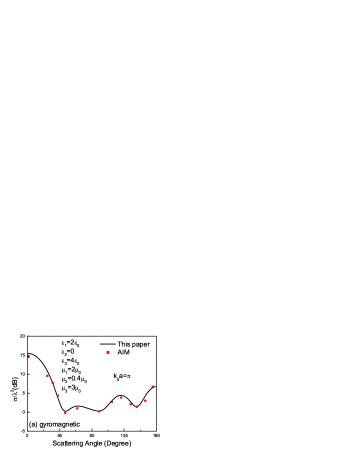
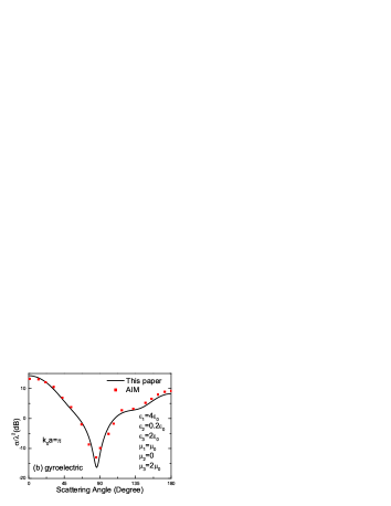
Figure 2: Radar cross sections (RCSs) versus the scattering angle (in degree) for (a) the gyromagnetic sphere and (b) the gyroelectric sphere. The comparisons in RCS results are made between our spectral-domain method (solid curve) and the AIM (square dot). The electronic size is fixed at $k_{0}a=\pi$.

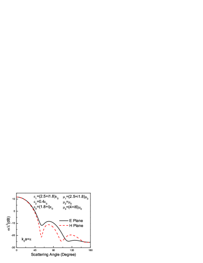
Figure 3: Radar cross sections (RCSs) versus scattering angle (in degrees): The electronic size is chosen as $k_{0}a=\pi$.

Then we study a more general case in Fig. 3 in which both material tensors ($\overline{\epsilon}$ and $\overline{\mu}$) are gyrotropic and lossy. The radar cross sections on $E$-plane and $H$-plane have been shown in Fig. 3. To the best of our knowledge, the scattering by such a general gyrotropic sphere has not been reported, except for its subcase of gyromagnetic spheres ref12b . Obviously, our model is more general in terms of the material complexity in Ref[13]. Our spectral-domain analysis is distinguished from the spatial-domain method in ref12b , and one can imagine that if the spatial method in Ref[13] is extended to study our general gyrotropic materials, the formulation would be lengthy due to the second tensor of permittivity. Hence, even for the general gyrotropic materials, our method results in simplified formulation.

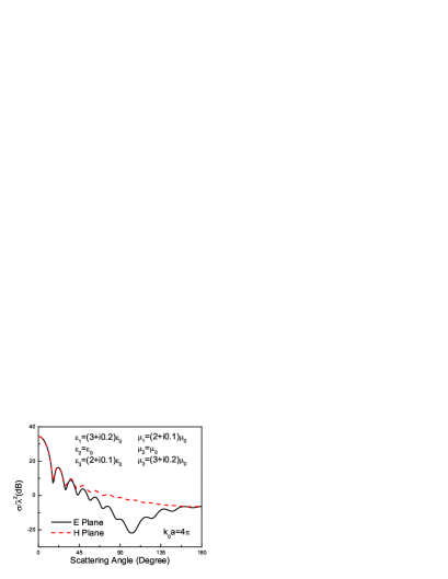
Figure 4: Radar cross sections (RCSs) versus scattering angle $\theta$ (in degree) in $E$-plane (solid curve) and and $H$-plane (dashed curve). The electric dimension is chosen to be $k_{0}a=4\pi$..

To illustrate the applicability of this analytical solution to the gyrotropic anisotropic sphere of electrically large size (for example, in the resonance region), the RCSs of a relatively large gyrotropic anisotropic sphere with loss are presented in Fig. 4. The lossy permittivity and permeability parameters are chosen as $\epsilon_{1}=(3+0.2i)\epsilon_{0}$, $\epsilon_{2}=\epsilon_{0}$, $\epsilon_{3}=(2+0.1i)\epsilon_{0}$, $\mu_{1}=(2+0.1i)\mu_{0}$, $\mu_{2}=\mu_{0}$, $\mu_{3}=(3+0.2i)\mu_{0}$. When the dimensions are increased, the convergence number ($N=24$ for the sphere $k_{0}a=4\pi$ in Fig. 4) is also increased.

IV Conclusions

In this paper, an analytical solution to the scattering by a general gyrotropic anisotropic sphere has been obtained. The method is developed based on the multipole expansion of the field along with the Fourier transform where the unknown angular spectrum amplitude is determined in spectral domain. The three-dimensional electromagnetic scattering of a plane wave by an gyrotropic anisotropic sphere has been theoretically formulated, physically characterized and numerically discussed. Numerical results for special cases are also obtained and verified by comparing with the results from the method of moments. The good agreement validates our spectral-domain scattering theory. By using our proposed theory, the scattering problems of the general optically anisotropic sphere can be analytically studied in spectral domain and RCSs can be readily computed. The analytical solution under arbitrary incident angle is still under investigation.

Appendix A Scattering coefficients of eigen-expansions in Eqs. (20) and (27)

$${\bf\mbox{\boldmath$F$}}^{e}_{q}(\theta,\phi)e^{i{\bf\mbox{\boldmath$k$}}_{q}\cdot{\bf\mbox{\boldmath$r$}}}\mbox{$$} = \mbox{$$}\sum_{mn}\Big{[}A^{e}_{mnq}(\theta_{k}){\bf\mbox{\boldmath$M$}}^{(1)}_{mn}({\bf\mbox{\boldmath$r$}},k_{q})$$ (A-1)

$$\mbox{$$}+B^{e}_{mnq}(\theta_{k}){\bf\mbox{\boldmath$N$}}^{(1)}_{mn}({\bf\mbox{\boldmath$r$}},k_{q})$$

$$\mbox{$$}+C^{e}_{mnq}(\theta_{k}){\bf\mbox{\boldmath$L$}}^{(1)}_{mn}({\bf\mbox{\boldmath$r$}},k_{q})\Big{]}e^{-im\phi_{k}}.\quad\quad$$

Because the spherical wave functions ${\bf\mbox{\boldmath$L$}}_{mn}({\bf\mbox{\boldmath$r$}},k)$, ${\bf\mbox{\boldmath$M$}}_{mn}({\bf\mbox{\boldmath$r$}},k)$, and ${\bf\mbox{\boldmath$N$}}_{mn}({\bf\mbox{\boldmath$r$}},k)$ form a complete set of orthogonal basis functions, we can employ them to expand any solutions uniquely, e.g.,

$$\widehat{x}e^{i{\bf\mbox{\boldmath$k$}}_{q}\cdot{\bf\mbox{\boldmath$r$}}}\mbox{$$}\ \ = \ \ \mbox{$$}\sum_{mn}\Big{[}a^{x}_{mn}(\theta_{k}){\bf\mbox{\boldmath$M$}}^{(1)}_{mn}({\bf\mbox{\boldmath$r$}},k_{q})+b^{x}_{mn}(\theta_{k})\quad\quad$$

$$\mbox{$$}\cdot{\bf\mbox{\boldmath$N$}}^{(1)}_{mn}({\bf\mbox{\boldmath$r$}},k_{q})+c^{x}_{mn}(\theta_{k}){\bf\mbox{\boldmath$L$}}^{(1)}_{mn}({\bf\mbox{\boldmath$r$}},k_{q})\Big{]},$$

$$\widehat{y}e^{i{\bf\mbox{\boldmath$k$}}_{q}\cdot{\bf\mbox{\boldmath$r$}}}\mbox{$$}\ \ = \ \ \mbox{$$}\sum_{mn}\Big{[}a^{y}_{mn}(\theta_{k}){\bf\mbox{\boldmath$M$}}^{(1)}_{mn}({\bf\mbox{\boldmath$r$}},k_{q})+b^{y}_{mn}(\theta_{k})$$

$$\mbox{$$}\cdot{\bf\mbox{\boldmath$N$}}^{(1)}_{mn}({\bf\mbox{\boldmath$r$}},k_{q})+c^{y}_{mn}(\theta_{k}){\bf\mbox{\boldmath$L$}}^{(1)}_{mn}({\bf\mbox{\boldmath$r$}},k_{q})\Big{]},$$

$$\widehat{z}e^{i{\bf\mbox{\boldmath$k$}}_{q}\cdot{\bf\mbox{\boldmath$r$}}}\mbox{$$}\ \ = \ \ \mbox{$$}\sum_{mn}\Big{[}a^{z}_{mn}(\theta_{k}){\bf\mbox{\boldmath$M$}}^{(1)}_{mn}({\bf\mbox{\boldmath$r$}},k_{q})+b^{z}_{mn}(\theta_{k})$$ (A-2)

$$\mbox{$$}\cdot{\bf\mbox{\boldmath$N$}}^{(1)}_{mn}({\bf\mbox{\boldmath$r$}},k_{q})+c^{z}_{mn}(\theta_{k}){\bf\mbox{\boldmath$L$}}^{(1)}_{mn}({\bf\mbox{\boldmath$r$}},k_{q})\Big{]}.$$

The coefficients in (A), i.e., $a^{p}_{mn}$, $b^{p}_{mn}$ and $c^{p}_{mn}$ (where $p=x,y,z$), are functions of $\theta_{k}$ and $\phi_{k}$. For the detailed expansion and discussion, the information can be found in ref13 . We provide only the coefficients of $A^{e}_{mnq}$, $B^{e}_{mnq}$ and $C^{e}_{mnq}$ used in the main text. From Eq. (II), we have

$${\bf\mbox{\boldmath$F$}}^{e}_{q}(\theta_{k},\phi_{k})={\bf\mbox{\boldmath$F$}}^{e1}_{q}(\theta_{k},\phi_{k})+{\bf\mbox{\boldmath$F$}}^{e2}_{q}(\theta_{k},\phi_{k}),$$ (A-3)

where

$${\bf\mbox{\boldmath$F$}}^{ep}_{q}(\theta_{k},\phi_{k})=F^{ep}_{qx}(\theta_{k},\phi_{k})\widehat{x}+F^{ep}_{qy}(\theta_{k},\phi_{k})\widehat{y}+F^{ep}_{qz}(\theta_{k},\phi_{k})\widehat{z}~{}~{}~{}~{}~{}~{}(p=1,~{}2)$$ (A-4)

with

$$F^{ep}_{qx}(\theta_{k},\phi_{k})\mbox{$$}\ \ = \ \ \mbox{$$}\left\{\begin{array}[]{ll}\displaystyle-\frac{\triangle_{1}}{\triangle}\sin\phi_{k},&p=1,\\ \displaystyle\frac{\triangle_{2}}{\triangle}\cos\phi_{k},&p=2;\end{array}\right.$$ (A-7)

$$F^{ep}_{qy}(\theta_{k},\phi_{k})\mbox{$$}\ \ = \ \ \mbox{$$}\left\{\begin{array}[]{ll}\displaystyle\frac{\triangle_{1}}{\triangle}\cos\phi_{k},&p=1,\\ \displaystyle\frac{\triangle_{2}}{\triangle}\sin\phi_{k},&p=2;\end{array}\right.$$ (A-10)

$$F^{ep}_{qz}(\theta_{k},\phi_{k})\mbox{$$}\ \ = \ \ \mbox{$$}\left\{\begin{array}[]{ll}0,&p=1,\\ 1,&p=2.\end{array}\right.$$ (A-13)

In the above equations, the intermediate parameters, $\triangle_{1}$, $\triangle_{2}$ and $\triangle$, are functions of only $\theta_{k}$ as given in Eq. (II). Then we can split the parameters as follows

$$A^{e}_{mnq}\mbox{$$}\ \ = \ \ \mbox{$$}A^{e1}_{mnq}+A^{e2}_{mnq},$$

$$B^{e}_{mnq}\mbox{$$}\ \ = \ \ \mbox{$$}B^{e1}_{mnq}+B^{e2}_{mnq},$$

$$C^{e}_{mnq}\mbox{$$}\ \ = \ \ \mbox{$$}C^{e1}_{mnq}+C^{e2}_{mnq},$$ (A-14)

and thus obtain ($p=1$ or 2)

$$A^{ep}_{mnq}e^{-im\phi_{k}}\mbox{$$}\ \ = \ \ \mbox{$$}F^{ep}_{qx}a^{x}_{mn}+F^{ep}_{qy}a^{y}_{mn}+F^{ep}_{qz}a^{z}_{mn},\quad\quad$$

$$B^{ep}_{mnq}e^{-im\phi_{k}}\mbox{$$}\ \ = \ \ \mbox{$$}F^{ep}_{qx}b^{x}_{mn}+F^{ep}_{qy}b^{y}_{mn}+F^{ep}_{qz}b^{z}_{mn},$$

$$C^{ep}_{mnq}e^{-im\phi_{k}}\mbox{$$}\ \ = \ \ \mbox{$$}F^{ep}_{qx}c^{x}_{mn}+F^{ep}_{qy}c^{y}_{mn}+F^{ep}_{qz}c^{z}_{mn}.$$ (A-15)

As a result, we can now obtain the expansion coefficients of ${\bf E}$-fields in a gyrotropic anisotropic medium, i.e., $A^{ep}_{mnq}$, $B^{ep}_{mnq}$ and $C^{ep}_{mnq}$ (where $q=1,2$), as follows:
for $p=1$ and $m\geq 0$

$$A^{e1}_{mnq}\mbox{$$}\ \ = \ \ \mbox{$$}i^{n}\frac{2n+1}{2n(n+1)}\frac{(n-m)!}{(n+m)!}\frac{\triangle_{1}}{\triangle}\Big{[}(n+m)(n-m$$

$$\mbox{$$}+1)P^{m-1}_{n}(\cos\theta_{k})-P^{m+1}_{n}(\cos\theta_{k})\Big{]},$$

$$B^{e1}_{mnq}\mbox{$$}\ \ = \ \ \mbox{$$}i^{n}\frac{1}{2n(n+1)}\frac{(n-m)!}{(n+m)!}\frac{\triangle_{1}}{\triangle}\Big{[}(n+1)(n+m)$$

$$\mbox{$$}\times(n+m-1)P^{m-1}_{n-1}(\cos\theta_{k})+(n+1)$$

$$\mbox{$$}\times P^{m+1}_{n-1}(\cos\theta_{k})+n(n\!-\!m\!+\!2)(n\!-\!m\!+\!1)$$

$$\mbox{$$}\times P^{m-1}_{n+1}(\cos\theta_{k})+nP^{m+1}_{n+1}(\cos\theta_{k})\Big{]},$$

$$C^{e1}_{mnq}\mbox{$$}\ \ = \ \ \mbox{$$}i^{n}\frac{1}{2k_{q}}\frac{(n-m)!}{(n+m)!}\frac{\triangle_{1}}{\triangle}\Big{[}(n+m)(n+m-1)$$ (A-16)

$$\mbox{$$}\times P^{m-1}_{n-1}(\cos\theta_{k})+P^{m+1}_{n-1}(\cos\theta_{k})$$

$$\mbox{$$}-(n-m+2)(n-m+1)P^{m-1}_{n+1}(\cos\theta_{k})$$

$$\mbox{$$}-P^{m+1}_{n+1}(\cos\theta_{k})\Big{]};$$

while for $p=1$ and $m>0$,

$$A^{e1}_{-mnq}\mbox{$$}\ \ = \ \ \mbox{$$}(-1)^{m}\frac{(n+m)!}{(n-m)!}A^{e1}_{mnq},$$

$$B^{e1}_{-mnq}\mbox{$$}\ \ = \ \ \mbox{$$}(-1)^{m+1}\frac{(n+m)!}{(n-m)!}B^{e1}_{mnq},\quad\quad$$

$$C^{e1}_{-mnq}\mbox{$$}\ \ = \ \ \mbox{$$}(-1)^{m+1}\frac{(n+m)!}{(n-m)!}C^{e1}_{mnq}.$$ (A-17)

Similarly, for $p=2$ and $m\geq 0$, we have

$$A^{e2}_{mnq}\mbox{$$}\ \ = \ \ \mbox{$$}i^{n+1}\displaystyle\frac{2n+1}{n(n+1)}\frac{(n-m)!}{(n+m)!}\Big{\{}\frac{\triangle_{2}}{2\triangle}\Big{[}(n\!+\!m)(n\!-\!m$$

$$\mbox{$$}+1)P^{m-1}_{n}(\cos\theta_{k})+P^{m+1}_{n}(\cos\theta_{k})\Big{]}$$

$$\mbox{$$}+mP^{m}_{n}(\cos\theta_{k})\Big{\}},$$

$$B^{e2}_{mnq}\mbox{$$}\ \ = \ \ \mbox{$$}i^{n+1}\displaystyle\frac{1}{n(n+1)}\frac{(n-m)!}{(n+m)!}\Big{\{}\frac{\triangle_{2}}{2\triangle}\Big{[}(n\!+\!1)(n\!+\!m)$$

$$\mbox{$$}\times(n\!+\!m\!-\!1)P^{m-1}_{n-1}(\cos\theta_{k})-(n+1)$$

$$\mbox{$$}\times P^{m+1}_{n-1}(\cos\theta_{k})+n(n\!-\!m\!+\!2)(n\!-\!m\!+\!1)$$

$$\mbox{$$}\times P^{m-1}_{n+1}(\cos\theta_{k})-nP^{m+1}_{n+1}(\cos\theta_{k})\Big{]}$$

$$\mbox{$$}+\Big{[}n(n-m+1)P^{m}_{n+1}(\cos\theta_{k})$$

$$\mbox{$$}-(n+1)(n+m)P^{m-1}_{n-1}(\cos\theta_{k})\Big{]}\Big{\}},$$

$$C^{e2}_{mnq}\mbox{$$}\ \ = \ \ \mbox{$$}i^{n+1}\displaystyle\frac{1}{k_{q}}\frac{(n-m)!}{(n+m)!}\Big{\{}\frac{\triangle_{2}}{2\triangle}\Big{[}(n+m)(n+m-1)$$ (A-18)

$$\mbox{$$}\times P^{m-1}_{n-1}(\cos\theta_{k})-P^{m+1}_{n-1}(\cos\theta_{k})$$

$$\mbox{$$}-(n-m+2)(n-m+1)P^{m-1}_{n+1}(\cos\theta_{k})$$

$$\mbox{$$}+P^{m+1}_{n+1}(\cos\theta_{k})\Big{]}-(2n+1)\cos\theta_{k}$$

$$\mbox{$$}\times P^{m}_{n}(\cos\theta_{k})\Big{\}};$$

while for $p=2$ and $m>0$,

$$A^{e2}_{-mnq}\mbox{$$}\ \ = \ \ \mbox{$$}(-1)^{m+1}\frac{(n+m)!}{(n-m)!}A^{e2}_{mnq},\quad\quad$$

$$B^{e2}_{-mnq}\mbox{$$}\ \ = \ \ \mbox{$$}(-1)^{m}\frac{(n+m)!}{(n-m)!}B^{e2}_{mnq},$$

$$C^{e2}_{-mnq}\mbox{$$}\ \ = \ \ \mbox{$$}(-1)^{m}\frac{(n+m)!}{(n-m)!}C^{e2}_{mnq}.$$ (A-19)

In a procedure similar to the above, the expansion coefficients of the ${\bf H}$-field eigenvector in gyrotropic anisotropic medium can be also obtained.

References

(1) A. Taflove and M. E. Brodwin, IEEE Trans. Microwave Theory Tech.
23, 623 (1975).
(2) R. D. Graglia, P. L. E. Uslenghi, and R. S. Zich, Proc. of IEEE 77, 750 (1989).
(3) W. X. Bao and K. Yasumoto, J. Appl. Phys. 82, 1996 (1997).
(4) N. A. Ozdemir and J.F. Lee, IEEE Trans. Magn. 44, 1398 (2008).
(5) V. V. Varadan, A. Lakhtakia, and V. K. Varadran, IEEE Trans. Antennas Propagat. 37, 800 (1989).
(6) D. R. Wyman, M. S. Patterson, and B. C. Wilson, J. Computational Phys. 81, 137 (1989).
(7)
S. N. Papadakis, N. K. Uzunoglu and C. N. Capsalis, J. Opt. Soc. Am.
A 7, 991 (1990).
(8) H. Hembd and H. Kschwendt, J. Computational Phys. 10, 534 (1972).
(9)
Y. Shi, J. Appl. Phys. 70, 3765 (1991).
(10)
Y. L. Geng, IET Microw. Antennas Propag. 2, 158 (2008).
(11)
Y. L. Geng, X. B. Wu, L. W. Li, and B. R. Guan, Phys. Rev. E
70, 0566609 (2004).
(12)
D. Sarkar and N. J. Halas, Phys. Rev. E 56, 1102 (1997).
(13) Z. Lin and S. T. Chui, Phys. Rev. E 69, 056614 (2004).
(14)W. C. Chew Waves and Fields in Inhomogeneous media, Van Nostrand, New York,
1990.
(15) M. Abramowitz and I. A. Stegun, Handbook of Mathematical Functions With Formulas, Graphs, and Mathematical Tables, Dover Publications, Inc., New York, 1972.
(16) L. Hu, L.-W. Li, and T.-S. Yeo, Progress In Electromagn. Res. 99, 21 (2009).
(17) C. Mei, Electromagnetic Scattering From an Arbitrarily Shaped Three Dimensional Inhomogeneous Bianisotropic Body, PhD Dissertation, Syraucuse University, US, December
2007.