Gene circuit designs for noisy excitable dynamics

Abstract

Certain cellular processes take the form of activity pulses that can be interpreted in terms of noise-driven excitable dynamics. Here we present an overview of different gene circuit architectures that exhibit excitable pulses of protein expression, when subject to molecular noise. Different types of excitable dynamics can occur depending on the bifurcation structure leading to the specific excitable phase-space topology. The bifurcation structure is not, however, linked to a particular circuit architecture. Thus a given gene circuit design can sustain different classes of excitable dynamics depending on the system parameters.

1 Introduction

Dynamical behavior is ubiquitous in gene regulatory processes. While many of the dynamical phenomena exhibited by genetic circuits take the form of periodic oscillations, in certain cases the behavior is governed by randomly occurring pulses of protein expression. Mathematically, this type of dynamics can be understood as an instance of excitability, by which a dynamical system with a stable fixed point is forced to undergo, when subject to a relatively small perturbation, a large excursion in phase space before relaxing back to the fixed point [1] (top panel in Fig. 1). This feature arises when the system is close to a bifurcation point beyond which the dynamics has the form of a limit cycle (bottom panel in Fig. 1).

Functionally, excitability provides cells with a mechanism to amplify molecular noise and transform it into a macroscopic cellular response. Biochemical activity pulses have been reported to exist in cAMP signaling in amoebae [2], response to DNA damage in human cells [3], competence in bacteria [4, 5], and differentiation priming in embryonic stem cells [6]. In a different (but still biological) context, electrical activity pulses in a specific cell type, namely neurons, have long been associated with excitable dynamics [7]. Within that context, early work by Hodgkin [8] identified two main different types of excitability on the basis of the frequency response of the neuron across a bifurcation leading from excitable to oscillatory behavior (Fig. 2). Type I excitability corresponds to a situation in which the limit cycle is born at the bifurcation with a frequency equal to zero, i.e. the oscillatory activity pulses become infinitely sparse as the bifurcation is approached (left panels in Fig. 2). In type II excitability, on the other hand, the limit cycle is born with a non-zero frequency (and thus with a finite period), as shown in the right panel of Fig. 2. The distinction is not purely academic: given that neurons encode information mainly in the timing between pulses, the two types of excitability correspond to two fundamentally different modes of information transmission [9]. Additionally, they exhibit distinct statistical features in their response to noise [9].

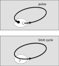
Figure 1: Schematic representation of excitable dynamics (top) and its associated limit-cycle behavior (bottom). The solid circle in the top plot represents the stable fixed point of the system. In this regime, large enough perturbations (starting at the empty circle in top panel) result in a large excursion through phase space before coming back to the stable state. Representation adapted from [7].

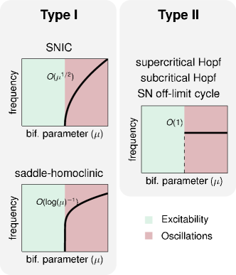
Figure 2: Frequency response to the increase of a given control parameter, for the two types of excitable behavior discussed in the text, as a bifurcation from excitability to oscillations is crossed. The different bifurcation types underlying the different scenarios are listed in top of each plot.

The two types of excitability shown in Fig. 2 are associated with different classes of bifurcation to oscillatory behavior. Two kinds of bifurcation lead to type I excitability. The first is a saddle-node on an invariant circle (SNIC) bifurcation, in which a stable node and a saddle point appear together on a limit cycle. In that regime, the trajectory along the remnant of the limit cycle delimits the excitable pulse. The second bifurcation leading to type I excitability is a saddle-homoclinic bifurcation, which occurs when a stable limit cycle collides with a saddle point, being transformed into a homoclinic orbit at the bifurcation point. Again this orbit delimits the excitable pulse. In both cases the existence of a saddle provides the system with a well defined excitability threshold, given by the stable manifold of the saddle. The two bifurcation scenarios are characterized by qualitatively distinct scaling relations of the frequency with respect to the control parameter [10], as specified inside the plots at the left column of Fig. 2.

Type II excitability, on the other hand, is associated with a Hopf bifurcation, either supercritical or subcritical, or to a saddle-node bifurcation occurring near (not on top of) a limit cycle. In the latter case, the saddle separates the stable fixed point from the periodic orbit, and again its stable manifold constitutes a separatrix that determines the excitability threshold. In the case of the Hopf bifurcation, on the other hand, it is not possible to define in a quantitative way an excitation threshold in phase space.

Given that the type of excitability determines the statistics of the noise-driven pulses, it is important to establish, in the context of gene regulation dynamics, the relationship between the gene circuit architecture and the phase-space topology resulting in excitability. A previous study [11] has linked the specific dynamical features of two-component genetic oscillators to the particular molecular implementation of one of the regulatory links, associating transcriptional regulation with type I dynamics, and post-translational regulation with type II. Here we show that both types of excitability are possible in both architectures, and add a third one that has been identified in bacteria, for which again both types of excitability are possible. Thus, our results indicate that circuit architecture does in principle not constrain the type of dynamics that the system exhibits. The three circuits under consideration are described in the next Section, followed in the subsequent Sections by detailed bifurcation analyses of the three systems for two parameter sets each, which lead to the two types of dynamics described above. Finally, in Section 6 we explore the parameter space to confirm that both types of excitable behaviors can be achieved for a wide range of parameter values.

2 A catalogue of excitable circuits

In what follows we will study the three circuits shown in Fig. 3. Circuit A has been identified as the core module underlying transient differentiation into competence in B. subtilis cells when placed under nutritional stress [4]. A protein x activates its own transcription and represses the transcription of a second protein y. The bistable switch on x resulting from the positive feedback loop is kept off by means of the protease P, which degrades x, but also y. This competitive degradation leads to excitable behavior, as shown in Sec. 3. The continuous description of this circuit’s dynamics in terms of two coupled ordinary equations for x and y is given below the circuit diagram in Fig. 3.

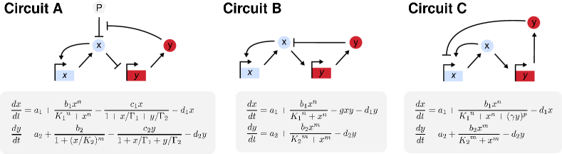
Figure 3: Three excitable circuits (top) and their corresponding continuous mathematical models (bottom). In the circuit diagrams, uppercase letters and circles represents proteins, and lowercase letters and rectangles denote genes.

The other two genetic circuits investigated in this work are two-component activator-repressor systems, in which the activator species forms a direct positive feedback loop through its auto-regulation and an indirect negative feedback loop by means of the activation of its repressor. Specifically, in both circuits B and C an activator protein x binds to and activates its own expression, and the expression of a repressor protein y. The repressor protein, in turn, inhibits the expression of the activator species in one of two ways: (i) post-translationally, by inactivating directly the activator protein (degrading it, for instance), such as in circuit B, or (ii) transcriptionally, by binding to the promoter of x and inhibiting its expression, which is the case of circuit C. The mathematical models of these two circuits are given below their corresponding diagrams in Fig. 3. These activator-repressor modules are very frequent in natural circuits. In particular, this is a generic circuit architecture for cell-cycle and circadian oscillators, which need to generate highly regular periodic activity. These two circuits have also been implemented synthetically. The post-translational activator-repressor module (circuit B) has been constructed synthetically in B. subtilis, where it has been shown to be functional in the development of competence [12], while the transcriptional activator-repressor module (circuit C) was built for instance in E. coli [13]. Additional synthetic versions of this latter type of circuit have been built that either include a negative self-feedback of the repressor on itself [14], or where the repressor action is mediated by quorum sensing [15].

In the next three Sections we analyze sequentially the potential dynamical regimes that these circuits exhibit, for different parameter values. As we will see, all three circuit architectures are able to display the two types of excitable dynamics represented in Fig. 2. To verify this, we will show the bifurcation diagrams leading to excitability in all cases, using the unregulated, basal expression of protein x as bifurcation parameter. A qualitative comparison between the excitable time traces generated by the discrete stochastic simulation of these models in the three circuits will be made.

3 Circuit A: a competitive degradation circuit

3.1 Type I excitability close to a saddle-homoclinic bifurcation

For the set of parameters given in Table 1 (determined in a previous work by comparison with experimental observations [5]), the competitive degradation circuit labeled as circuit A in Fig. 3 exhibits excitable dynamics. Figure 4(a) shows the phase portrait of the deterministic model of that circuit (see equations in Fig. 3) in the excitable regime.

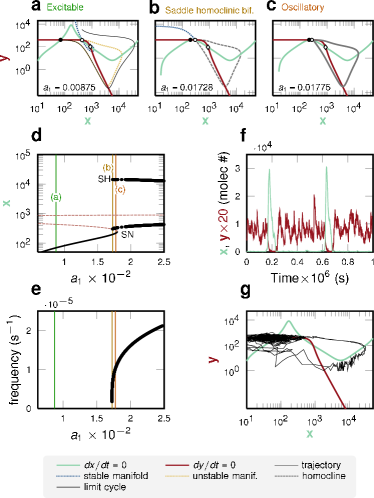
Figure 4: Type I excitability close to a saddle-homoclinic bifurcation in circuit A. (a-c) Phase portraits for three values of the parameter $a_{1}$. The green and red lines represent the nullclines of $x$ and $y$. The stable and unstable manifolds of the saddle point are represented by blue and yellow dotted lines respectively. (d) Bifurcation diagram of the system for varying $a_{1}$. Vertical lines correspond to the values of $a_{1}$ for which the phase portraits are shown in plots (a-c). (e) Frequency of the oscillations versus $a_{1}$. (f) Time traces of protein levels for both species in the gene circuit, as generated from stochastic simulations of its constituent reactions. (g) Corresponding stochastic trajectory in the phase plane. The values of the parameters used here are given in Table 1.

	Circuit A		Circuit B		Circuit C
	Type I	Type II	Type I	Type II	Type I	Type II
$a_{1}$	0.00875 $\,\text{nM}/\,\text{s}$	0.016 $\,\text{nM}/\,\text{s}$	0.00875 $\,\text{nM}/\,\text{s}$	0.005 $\,\text{nM}/\,\text{s}$	0.15 $\,\text{nM}/\,\text{s}$	0.147 $\,\text{nM}/\,\text{s}$
$a_{2}$	0 $\,\text{nM}/\,\text{s}$	0 $\,\text{nM}/\,\text{s}$	0.075 $\,\text{nM}/\,\text{s}$	0.025 $\,\text{nM}/\,\text{s}$	0.05 $\,\text{nM}/\,\text{s}$	0 $\,\text{nM}/\,\text{s}$
$b_{1}$	7.5 $\,\text{nM}/\,\text{s}$	6 $\,\text{nM}/\,\text{s}$	7.5 $\,\text{nM}/\,\text{s}$	15 $\,\text{nM}/\,\text{s}$	7.5 $\,\text{nM}/\,\text{s}$	7 $\,\text{nM}/\,\text{s}$
$b_{2}$	0.06 $\,\text{nM}/\,\text{s}$	0.3 $\,\text{nM}/\,\text{s}$	2.5 $\,\text{nM}/\,\text{s}$	0.8 $\,\text{nM}/\,\text{s}$	10 $\,\text{nM}/\,\text{s}$	0.8 $\,\text{nM}/\,\text{s}$
$c_{1}$	0.001 $\,\text{nM}/\,\text{s}$	0.001 $\,\text{nM}/\,\text{s}$	—	—	—	—
$c_{2}$	0.001$\,\text{nM}/\,\text{s}$	0.001 $\,\text{nM}/\,\text{s}$	—	—	—	—
$d_{1}$	0.0001 $\,\text{s}^{-1}$	0.0001 $\,\text{s}^{-1}$	0.0001 $\,\text{s}^{-1}$	$5\cdot 10^{-5}$ $\,\text{s}^{-1}$	0.000386 $\,\text{s}^{-1}$	0.0004$\,\text{s}^{-1}$
$d_{2}$	0.0001 $\,\text{s}^{-1}$	0.0001 $\,\text{s}^{-1}$	0.0001 $\,\text{s}^{-1}$	$5\cdot 10^{-5}$ $\,\text{s}^{-1}$	$3.86\cdot 10^{-5}$ $\,\text{s}^{-1}$	$4\cdot 10^{-5}$ $\,\text{s}^{-1}$
$g$	—	—	$4\cdot 10^{-8}$ $(\,\text{nM}\cdot\,\text{s})^{-1}$	$2.5\cdot 10^{-7}$ $(\,\text{nM}\cdot\,\text{s})^{-1}$	—	—
$K_{1}$	5000  nM	4000  nM	5000  nM	3000  nM	5000  nM	5000  nM
$K_{2}$	833  nM	500  nM	2500  nM	750  nM	75000  nM	2000  nM
$\Gamma_{1}$	25000  nM	20000  nM	—	—	—	—
$\Gamma_{2}$	20  nM	100  nM	—	—	—	—
$\gamma$	—	—	—	—	2	0.5
$n$	2	2	2	2	2	2
$m$	5	2	2	2	2	2
$p$	—	—	—	—	2	2

Table 1: Parameter values used in the deterministic equations of the three gene regulatory circuits. For these sets of parameters, the circuits exhibit either type I or type II excitability.

The plot depicts the $x$ and $y$ nullclines (in green and red, respectively, in plots a-c and g), the stable and unstable manifolds of the saddle, and a sample deterministic trajectory (thin black line, see figure legend for a description of the other lines used). The excitable regime is characterized by a stable fixed point with low levels of x (black circle) that coexists with two unstable fixed points, a saddle (white circle) and a spiral (white diamond). The upper part of the stable manifold of the saddle (blue dotted curve) is the excitability threshold: any trajectory starting at the right of that manifold is forced to go through a large excursion in phase space (note the logarithmic scale in the plot’s axes) towards increasing $x$, leading to an excitability pulse.

As the basal expression $a_{1}$ of x increases, a saddle-homoclinic bifurcation (SH) takes place, at which the saddle point collides with a stable limit cycle that surrounds the unstable spiral point (Fig. 4b), giving rise to a homoclinic orbit (dashed grey line). For a small parameter range the limit cycle coexists with the stable node and the saddle (Fig. 4c), until both collide in a saddle-node (SN) bifurcation, after which the limit cycle (solid grey line) is the only attractor of the system. This can be seen in the bifurcation diagram shown in Fig. 4(d), which represents the limit cycle as a thick black line, and the stable and unstable fixed points as thin solid black and dashed red lines, respectively.

The corresponding behavior of the frequency of the oscillations with respect to the parameter $a_{1}$ is represented in Fig. 4(e). The plot shows that the oscillation frequency at the right of the saddle-homoclinic bifurcation tends to zero as the bifurcation is approached, which is a clear hallmark of type I excitable behavior (the frequency values close to zero are not shown due to numerical constraints). Time traces generated via stochastic simulations of the set of reactions forming the circuit, using the standard Gillespie method [16], are displayed in Fig. 4(f). The figure shows that the two species taking part in the dynamics are anticorrelated, with wide pulses of activity of x leading to dips in the amount of y protein present in the cell. The corresponding trajectory in phase space is shown in Fig. 4(g). Previous work [12] has revealed that this circuit design leads to highly variable pulse durations, which have the physiological function of allowing cells to cope with the natural unpredictability associated with low extracellular DNA levels to which B. subtilis cells are subject in the presence of nutritional stress.

3.2 Type II excitability close to a supercritical Hopf bifurcation

A different parameter set (see Table 1) leads to a completely different bifurcation scenario that also leads to excitability. The phase portrait of the system for the excitable regime in this case is shown in Fig. 5(a). The nullclines now cross only once, corresponding to a stable spiral point which is the rest state of the excitable dynamics. Even though there is no saddle here that helps us define an excitability threshold, a large enough perturbation away from the stable fixed point is able to elicit a large excursion in phase space, an example of which is shown as a thin black line in Fig. 5(a).

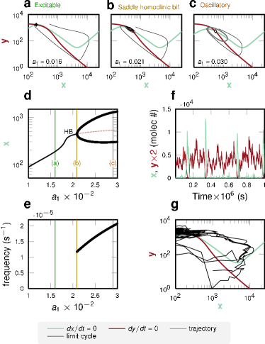
Figure 5: Type II excitability close to a supercritical Hopf bifurcation in circuit A. The meaning of the plots is the same as in Fig. 4.

As the value of $a_{1}$ increases, the system undergoes a supercritical Hopf bifurcation (Fig. 5b) that destabilizes the spiral point and generates a stable limit cycle around it, which is born with zero amplitude, as can be seen in the bifurcation diagram of Fig. 5(d). Beyond the Hopf bifurcation, the system exhibits a well-developed stable limit cycle (Fig. 5c). Interestingly, certain perturbations of this limit cycle evoke large-amplitude excursions in phase-space, similarly to what happens in the standard excitable regime shown in Fig. 5(a). An example of such an excursion is shown by a thin solid line in Fig. 5(c). This regime can be interpreted as an excitable dynamics with subthreshold oscillations, something that is well-known to exist in the context of neural systems [17].

The frequency response of the circuit to a variation in $a_{1}$ is shown in Fig. 5(e). In this case one can see that the frequency remains finite at the bifurcation, which is characteristic of type II excitability, as mentioned above. This behavior is a direct consequence of the fact that the underlying bifurcation bridging excitability and oscillatory dynamics is a supercritical Hopf bifurcation. Typical time traces of the protein levels of x and y are shown in Fig. 5(f). Again, as in the previous Section, there is anticorrelation between the two proteins during the excitation pulse, although in contrast with the previous case, there is a large variability in the pulse amplitude. This is due to the fact that the pulse trajectories in this case depend much more strongly on the initial conditions of the pulse than in the case of the previous Section (compare Figs. 4g and 5g).

4 Circuit B: a post-translational activator-repressor circuit

4.1 Type I excitability close to a SNIC bifurcation

We now turn to the activator-repressor circuits, beginning with the post-translational one, in which protein y represses x by interfering directly, at the protein level, with its activity (for example by degrading it). For a set of parameters (given in Table 1) that successfully reproduce experimental observations [12], this system also behaves in an excitable manner. The corresponding phase portrait is shown in Fig. 6(a). Again, as in Sec. 3.1, the system has three fixed points, only one of which is stable. Perturbations away from this stable fixed point, that take the trajectory past the stable manifold of the saddle (which acts again as an excitability threshold), will cause a large excursion in phase space surrounding the two unstable fixed points, as represented by a thin black line in the figure.

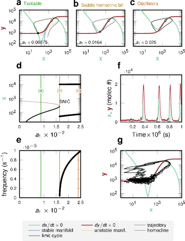
Figure 6: Type I excitability close to a SNIC bifurcation in circuit B. The meaning of the plots is the same as in Fig. 4.

As the value of the parameter $a_{1}$ increases, a global bifurcation will again, as in Sec. 3.1, generate a limit cycle with a finite amplitude (Fig. 6b). In contrast with the case of Sec. 3.1, however, the bifurcation is now a saddle-node on an invariant circle (SNIC), since the stable node and the saddle that exist in the excitable regime collide with each other and annihilate exactly on top of the newly born limit cycle. The resulting fully developed limit cycle that exists after the bifurcation is represented in Fig. 6(c), and the corresponding bifurcation diagram is shown in Fig. 6(d). The SNIC bifurcation is revealed in this plot by the simultaneous occurrence of the saddle-node (SN) bifurcation, through which the stable and unstable fixed-point branches annihilate with each other, and the appearance of the stable limit cycle, at exactly the same value of $a_{1}$.

As summarized in the scheme of Fig. 2, SNIC bifurcations are associated with type I excitable dynamics, for which the frequency tends to zero at the bifurcation point. This fact is shown in Fig. 6(e). Time traces and phase-plane trajectories corresponding to the excitable regime are presented in Figs. 6(f) and (g). Note that in this case there is a positive correlation between the two protein species of the circuit, with the repressor slightly tailing behind (shutting off, in fact) the activator. The positive correlation is a reflection that the trajectory in phase space is counterclockwise (see Fig. 6a). Again, as in the case of circuit A (Sec. 3.1), there is little dispersion in the pulse amplitudes. In contrast with that other circuit, however, the dispersion in the pulse widths is known to be here much smaller [12].

4.2 Type II excitability close to a subcritical Hopf bifurcation

The post-translational activator-repressor circuit represented as circuit B in Fig. 3 can also exhibit type II dynamics. The situation is represented in Fig. 7, for which the corresponding parameters are again given in Table 1.

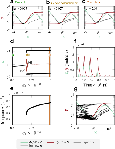
Figure 7: Type II excitability close to a subcritical Hopf bifurcation in circuit B. The meaning of the plots is the same as in Fig. 4.

As shown in Fig. 7(a), the excitable regime is characterized by a single fixed point. The cubic nullcline of the activator and the monotonically increasing nullcline of the inhibitor make this system analogous to a FitzHugh-Nagumo model. As in that model, the dynamics exhibit separation of time scales between the two species, in such a way that the dynamics of the activator is much faster than that of the inhibitor. This is reflected in a quick entry into the excitable pulse and a slower exit, the latter governed by the final part of the trajectory in which the system approaches the fixed point again by slowly sliding down the left branch of the activator nullcline (see Fig. 7a). In this case, however, the separation of time scales is not imposed by tuning the parameters (both species have the same linear degradation terms), but effective and due to the post-translational inactivation of x by y. As the parameter $a_{1}$ increases, excitability is once more lost, this time via a subcritical Hopf bifurcation in which the fixed point loses stability via a collision with an unstable limit cycle (Fig. 7b). This unstable invariant set was previously generated via a fold limit cycle (FLC) bifurcation, together with a stable limit cycle which becomes the only stable attractor (Fig. 7c) after the subcritical Hopf bifurcation occurs. The situation is summarized in the bifurcation diagram shown in Fig. 7(d) where the thick red line represents the unstable limit cycle branch.

The subcritical Hopf bifurcation described above leads to type II dynamics, which we remind is characterized by the fact that the frequency remains finite at the bifurcation. This is shown in Fig. 7(e). Finally, Figs. 7(f) and (g) shows sample trajectories of the system as generated from stochastic simulations. In this case, as in Sec. 3.2, the variability of pulse amplitudes is slightly higher than for type I excitability.

5 Circuit C: a transcriptional activator-repressor circuit

5.1 Type I excitability close to a SNIC bifurcation

We now substitute the post-translational repression of x by y for a transcriptional regulation, in which the repressor competitively inhibits expression of the activator by binding to its promoter. In this case the system can also behave as an excitable system, as shown in Fig. 8(a). As in the previous examples of type I excitability discussed above (Secs. 3.1 and 4.1), this system has three fixed points, only one of them being stable. Once more the stable manifold of the saddle defines the excitability threshold, beyond which a pulse of excitability is triggered. An increase in $a_{1}$ leads to a SNIC bifurcation in which the stable node and the saddle collide and annihilate at the same location at which a limit cycle appears (Fig. 8b). The corresponding bifurcation diagram is shown in Fig. 8(d).

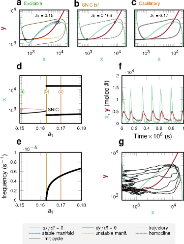
Figure 8: Type I excitability close to a SNIC bifurcation in circuit C. The meaning of the plots is the same as in Fig. 4.

As expected, the frequency of the limit cycle (shown in Fig. 8c) decays to zero as the bifurcation is approached, as displayed in Fig. 8(e). The time traces (Fig. 8f) and corresponding trajectory in phase space (Fig. 8g) show that the two species are positively correlated, and that there are slight variations in the pulse amplitudes (in contrast with the other examples of type I dynamics discussed above, where the variability in amplitude was basically absent).

5.2 Type II excitability close to a subcritical Hopf bifurcation

Finally, we show that the transcriptional version of the activator-repressor circuit can also display type II dynamics. Figure 9 shows the behavior of the circuit for the parameters given in Table 1. As in the FitzHugh-Nagumo model, we have to assume a clear separation of time scales between the activator and repressor, the former being much faster than the latter. The phase portrait corresponding to the excitable regime, shown in Fig. 9(a), is again analogous to that exhibited by a standard FitzHugh-Nagumo model. No well-defined excitability threshold exists, but perturbations sufficiently far away from the rest state take the system to the excited branch of the activator nullcline (right branch). The bifurcation is very similar to the one exhibited by the post-translational activator-repressor circuit of Sec. 4.2. As $a_{1}$ increases, the rest state loses stability via a subcritical Hopf bifurcation (Fig. 9b) that generates a stable limit cycle (Fig. 9c).

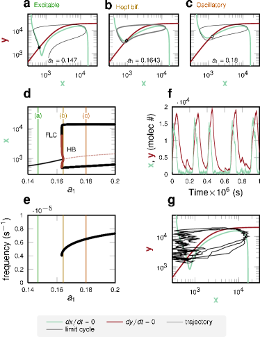
Figure 9: Type II excitability close to a subcritical Hopf bifurcation in circuit C. The meaning of the plots is the same as in Fig. 4.

The bifurcation plot (Fig. 9d) reveals that the limit cycle is born via a fold limit cycle bifurcation (FLC) that is closely followed by the above-mentioned subcritical Hopf bifurcation (HB), after which the limit cycle is the only stable attractor of the system. Excitable dynamics occurs before the FLC bifurcation. The period behaves in a manner consistent with a type II dynamics, remaining different from zero up to the bifurcation point. Typical time traces and phase-space trajectories are shown in Figs. 9(f) and (g), respectively.

6 Excitability in parameter space

We have shown that all three circuits can exhibit both types of excitability regimes depending on specific values of the kinetic parameters. In this section we show that the parameters used in each case (Table 1) are not exceptional and that both types of excitability are expected in these circuits. For each of the three circuits, we partially explore parameter space between the parameters sets used in the previous sections (see Table 1). Specifically, if $\boldsymbol{\pi}_{I}$ and $\boldsymbol{\pi}_{II}$ are the parameter vectors used for type I and type II excitability, we can map a control parameter $\alpha$ to the linear combination of these two parameter vectors, $\alpha\mapsto\boldsymbol{\pi}(\alpha)=(1-\alpha)\cdot\boldsymbol{\pi}_{I}+\alpha\cdot\boldsymbol{\pi}_{II}$. This new parameter allows us to track the transition from type I excitability at $\alpha=0$ to type II excitability at $\alpha=1$, and will give us a sense of how general these regimes are in each of the circuits studied here. We have restricted the parameter space scan to values of $\alpha$ for which all the parameters were strictly positive. This restriction defines the range of values that $\alpha$ can take to $(-0.25,1.667)$ for circuit A, $(-0.19,1.429)$ for circuit B, and $(-27.57,1)$ for circuit C. Figure 10 shows a two-dimensional bifurcation diagram for the parameters $\alpha$ and $a_{1}$ for the three circuits. The transition from type I to type II excitability in circuit A is shown in Fig. 10(a). Type I excitability is maintained as we move from the set of parameters used in Sec. 3.1 ($\alpha=0$, black circle) towards the set of parameters used in Sec. 3.2 ($\alpha=1$, white square). In this Figure, the left-most saddle-node (SN) branch is associated with type I excitable dynamics (Fig. 4). As $\alpha$ increases, the complementary SN branch appears and both eventually collide in a cusp point. Just before this codimension-2 bifurcation occurs, a Bogdanov-Takens bifurcation takes place in the lowest SN branch ($\alpha\approx 0.865$) and gives rise to the Hopf bifurcation leading to type II excitability. Thus, in this circuit excitability is preserved for all values of $\alpha$, and both types of excitable dynamics are possible in a wide range of parameters. The same is true for circuit B (Fig. 10b) where the SNIC bifurcation responsible of type I excitability is annihilated in a cusp point at $\alpha\approx 0.1748$ and the nascent subcritical Hopf bifurcation allows again for type II excitability. Finally, in Circuit C, type I dynamics occupies almost the whole scanned parameter range (see Fig. 10c), while type II dynamics is relegated to a marginal region. In our opinion, this is a limitation of this parameter scanning procedure rather than an imprint of the exceptionality of the type II regime in this circuit. The separation of time scales required for the excitability in this regime plus the large difference in some of the parameter values between the two regimes (e.g. $K_{2}$), makes it difficult to stay in type II excitability while decreasing from $\alpha=1$ to 0. We have observed that other parameter sets lead to type II dynamics in this circuit (data not shown), but this parameter scanning strategy fails in those cases.

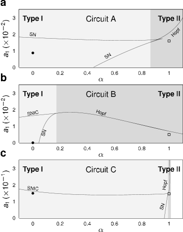
Figure 10: Bifurcation lines in the parameter space formed by $\alpha$ and $a_{1}$ for the three circuits (see main text). Clear grey (dark grey) areas correspond to the values of $\alpha$ for which the circuits exhibits type I (type II) excitability. Black circles denote the sets of parameters used in this text for type I dynamics, and white squares denote parameters for type II behavior.

7 Discussion

Relating structure and function is an outstanding problem in biology. The design principles underlying such a mapping can be revealed by means of design space representations [18]. In some cases, multiple circuit architectures can be associated with a single cellular function [19]. Here we have presented a collection of three gene-circuit designs that are able to exhibit excitable dynamics. All three architectures are known to exist in nature, and in some cases excitable dynamics has been observed experimentally. We were interested in determining whether a specific circuit type was necessarily associated with a given type of excitable dynamics, given that two distinct types are known to exist with different dynamical and statistical properties of the generated pulses. Our study shows that this is not the case, but that rather all types of circuits can generate both types of excitable behavior for a wide range of parameter values (at least in circuits A and B).

This type of design degeneracy can be expected to be very common in natural systems. Theoretical studies have found this to be the case in noise-buffering circuits [20] and pattern-forming circuits in development, for functions such as segmentation [21] and single-stripe formation [19]. Recent studies [12, 22] have shown that such a dynamical degeneracy can be lifted by noise, provided the different circuit architectures involved are associated with different phase relations between the circuit components: if the circuit topology is such that the proteins are anti-correlated, one of them will be always occurring in low numbers and will thus be subject to large fluctuations, so that the overall amount of noise in the system will be high. On the other hand, if the topology is such that the proteins are correlated, the levels of both proteins will be high or low simultaneously, and therefore the amount of noise will fluctuate in time inversely with the protein levels. In that way, noise propagates in different ways through the different circuit designs, and provides the system with specific functional properties that most likely act as fitness determinants in the evolution of a given molecular circuitry to perform a desired cellular function [12, 22].

On the other hand, the fact that a given circuit can have different dynamical behaviors would allow evolutionary pressures to shape the specific dynamical response of the cell (for instance in terms of their noise level) without having to modify the circuit’s topology. Hopefully the systematic dynamical study presented here could help in establishing how such these selection processes take place in other excitable cellular functions.

References

- [1] B. Lindner, J. García-Ojalvo, A. Neiman, L. Schimansky-Geier, Effects of noise in excitable systems, Physics Reports 392 (2004) 321–424.
- [2] T. Hofer, J. A. Sherratt, P. K. Maini, Dictyostelium discoideum: Cellular self-organization in an excitable biological medium, Proc. Royal Soc. London B 259 (1995) 249–257.
- [3] G. Lahav, N. Rosenfeld, A. Sigal, N. Geva-Zatorsky, A. J. Levine, M. B. Elowitz, U. Alon, Dynamics of the p53-mdm2 feedback loop in individual cells, Nat Genet 36 (2004) 147–50.
- [4] G. M. Süel, J. Garcia-Ojalvo, L. Liberman, M. Elowitz, An excitable gene regulatory circuit induces transient cellular differentiation, Nature 440 (2006) 545–550.
- [5] G. M. Süel, R. P. Kulkarni, J. Dworkin, J. Garcia-Ojalvo, M. B. Elowitz, Tunability and Noise Dependence in Differentiation Dynamics, Science 315 (2007) 1716–1719.
- [6] T. Kalmar, C. Lim, P. Hayward, S. Muñoz-Descalzo, J. Nichols, J. Garcia-Ojalvo, A. Martinez Arias, Regulated fluctuations in Nanog expression mediate cell fate decisions in embryonic stem cells, PLoS Biol 7 (2009) e1000149.
- [7] E. M. Izhikevich, Dynamical Systems in Neuroscience: The Geometry of Excitability and Bursting, The MIT Press, 2006.
- [8] A. L. Hodgkin, The local electric changes associated with repetitive action in a non-medullated axon, J. Physiol. 107 (1948) 165–181.
- [9] M. St-Hilaire, A. Longtin, Comparison of coding capabilities of type I and type II neurons, J Comput Neurosci 16 (2004) 299–313.
- [10] S. H. Strogatz, Nonlinear Dynamics And Chaos: With Applications To Physics, Biology, Chemistry, And Engineering (Studies in Nonlinearity), 1st Edition, Studies in nonlinearity, Perseus Books Group, 1994.
- [11] R. Guantes, J. F. Poyatos, Dynamical principles of two-component genetic oscillators, PLoS Comput Biol 2 (2006) e30.
- [12] T. Çağatay, M. Turcotte, M. Elowitz, J. Garcia-Ojalvo, G. Süel, Architecture-dependent noise discriminates functionally analogous differentiation circuits, Cell 139 (2009) 512–522.
- [13] M. R. Atkinson, M. A. Savageau, J. T. Myers, A. J. Ninfa, Development of genetic circuitry exhibiting toggle switch or oscillatory behavior in Escherichia coli, Cell 113 (2003) 597–607.
- [14] J. Stricker, S. Cookson, M. R. Bennett, W. H. Mather, L. S. Tsimring, J. Hasty, A fast, robust and tunable synthetic gene oscillator, Nature 456 (2008) 516–9.
- [15] T. Danino, O. Mondragón-Palomino, L. Tsimring, J. Hasty, A synchronized quorum of genetic clocks, Nature 463 (2010) 326–30.
- [16] D. T. Gillespie, Exact stochastic simulation of coupled chemical reactions, J. Phys. Chem. 81 (1977) 2340–2361.
- [17] B. Sancristóbal, J. M. Sancho, J. Garcia-Ojalvo, Phase-response approach to firing-rate selectivity in neurons with subthreshold oscillations, Phys. Rev. E 82 (2010) 041908.
- [18] M. A. Savageau, P. M. Coelhoa, R. A. Fasani, D. A. Tolla, A. Salvador, Phenotypes and tolerances in the design space of biochemical systems, Proc Natl Acad Sci U S A 106 (2009) 6435–40.
- [19] J. Cotterell, J. Sharpe, An atlas of gene regulatory networks reveals multiple three-gene mechanisms for interpreting morphogen gradients, Mol Sys Biol 6 (2010) 425.
- [20] G. Hornung, N. Barkai, Noise propagation and signaling sensitivity in biological networks: a role for positive feedback, PLoS Comp Biol 4 (2008) e8.
- [21] W. Ma, L. Lai, Q. Ouyang, C. Tang, Robustness and modular design of the Drosophila segment polarity network, Mol Sys Biol 2 (2006) 70.
- [22] M. Kittisopikul, G. M. Süel, Biological role of noise encoded in a genetic network motif, Proc Natl Acad Sci U S A 107 (2010) 13300–5.