THE ENERGY LEVEL SHIFTS, WAVE FUNCTIONS
AND THE PROBABILITY CURRENT DISTRIBUTIONS
FOR THE BOUND SCALAR AND SPINOR PARTICLES
MOVING IN A UNIFORM MAGNETIC FIELD

V. N. Rodionov, G. A. Kravtsova,

We discuss the equations for the bound one-active electron states based on the analytic solutions of the Schrodinger and Pauli equations for a uniform magnetic field and a single attractive $\delta({\bf r})$-potential. It is vary important that ground electron states in the magnetic field differ essentially from the analogous state of spin-$0$ particles, whose binding energy was intensively studied more than forty years ago. We show that binding energy equations for spin-$1/2$ particles can be obtained without using the language of boundary conditions in the $\delta$-potential model developed in pioneering works. We use the obtained equations to calculate the energy level displacements analytically and demonstrate nonlinear dependencies on field intensity. We show that the magnetic field indeed plays a stabilizing role in considered systems in a case of the weak intensity, but the opposite occurs in the case of strong intensity. These properties may be important for real quantum mechanical fermionic systems in two and three dimensions. We also analyze the exact solution of the Pauli equation for an electron moving in the potential field determined by the three-dimensional $\delta$-well in the presence of a strong magnetic field. We obtain asymptotic expressions for this solution for different values of the problem parameters. In addition, we consider electron probability currents and their dependence on the magnetic field. We show that including the spin in the framework of the nonrelativistic approach allows correctly taking the effect of the magnetic field on the electric current into account. The obtained dependencies of the current distribution, which is an experimentally observable quantity, can be manifested directly in scattering processes, for example.

Keywords:  bound electron, magnetic field, current probability distribution

1 Formulation of the problem

The effect of an external electromagnetic field on nonrelativistic charged particles systems (such as atoms, ions, and atomic nuclei) has long been investigated systematically (see, e.g., [2]-[16] ). Although this problem has a long history, a set of questions still requires additional study. For example, a systematic analysis of the bound states of spin-1/2 particles in an intense magnetic field has been lacking until now. We note that the basic results in the case of spinless particles were obtained using analytic solutions in nonperturbative mathematical treatments. As usual, the exact solutions of Schrödinger equations with Hamiltonians taking a particle bound by short-range potential in the presence of external fields into account are used. Furthermore, there is a rather common opinion that the role of the magnetic field in decays of quasistationary states is invariably stabilizing [4], [15], [16]. This view arises because the spinor states of electrons in an external electromagnetic field are usually neglected in nonrelativistic treatments, which is often inadequate [17], [18]. In this paper, we treat an essential part of these problems.

We consider charged spin-$0$ and spin-$1/2$ particles bounded by a short-range potential ($\delta$ potential) and located in an external stationary magnetic field with an arbitrary intensity. We note that the zero-radius potential is a widespread approximation for a multielectron atom field and especially for a negative ion field [13], [19]. Energy level displacements can be seen for the particle in a $\delta$ potential and a magnetic field. The binding-energy equation is most appropriate for the investigating such states([5], [13], [20]).

When an electron moves in a uniform magnetic field oriented in the $z$ direction, the quantum mechanical system is invariant with respect to the $z$ axis. The system then becomes essentially two-dimensional in the $xy$ plane. Many physical phenomena in axially symmetric quantum systems of electrically charged fermions (the quantum Hall effect [21], high-temperature superconductivity [22], various film defects [23], etc.) can be effectively studied using the nonrelativistic equations of motion in 2+1 dimensions. A number of effects in constant magnetic fields, including certain types of doped two-dimensional semimetals, can be described using the Dirac equation in 2+1 dimensions [24], [25]. But there are many physical phenomena that occur in three-dimensional space [26], [27]. In this paper, we investigate the effect of a stationary uniform magnetic field on localized electron states in $2+1$ and 3+1 dimensions (see also  [28], [29]).

The effects of external electromagnetic fields on bound nonrelativistic charged particles have already been studied systematically in detail over several decades (see, e.g., [16], [17], [30]). But although this problem has a very long history, several problems still need additional study. In particular, such problems include analyzing the effect of a strong magnetic field on bound charged particles with their spin states taken correctly into account.

There is a widespread opinion that consistently including the charged-particle spin is required only in studying relativistic effects. But this is not always the case for a strong magnetic field, as shown in [17], [31]. We note that efforts to analyze spin effects in the nonrelativistic approximation were made many times. Models precisely taking the effect of the field on the particle into account were used for this purpose. We emphasize that the wide experience in describing spinless particles bound by the $\delta$-like potential in strong electromagnetic fields has been acquired precisely because the nonperturbative mathematical approach was used. Developed methods based on the exact analytic solutions of the Schrödinger equation [16], [30], [32] were also used to study processes taking particle spins into account. But because mathematical estimates are complicated in the case of spinning particles, the obtained conclusions are not always sufficiently convincing. In our opinion, the papers [28], [31], [33], where the effects of the field on the behavior of spinning and scalar particles were compared, are most correct from the standpoint of the necessity to take particle spins into account. For these purposes, the solutions of the Pauli equations, together with the solutions of the Schrödinger equation, were also used in the indicated papers. We here consider the effects produced by the action of a strong constant uniform magnetic field on an electron bound by a short-range potential.

Under the action of the field, electron energy levels are shifted by a quantity determined from the transcendental equation for the energy. We note that this problem was analyzed in the case of a scalar particle in [32]. A similar problem for the electron in the magnetic field with its spin states taken into account was correctly solved in [28] quite recently.

Our main purpose is to derive equations for the binding energy of a fermion in a field containing an attractive singular potential and a stationary external magnetic field in the two- and three-dimensional cases. We apply standard quantum mechanical methods using the expansion of the unknown wave function in a series at the eigenfunctions obtained for the fermionic system in the pure magnetic field. This method was used to study some physical examples of the effect of a constant magnetic field on charged particles bound by a single attractive $\delta$ potential [34], [35]. This formalism differs in principle from the traditional derivation of wave functions in similar problems using the boundary condition typical for the $\delta$ potential [5], [6], [15], [16].

It is very important that our approach permits developing a consistent investigation of the spin effects arising in an external magnetic field. An exact analytic expression for the wave function of a charged scalar particle in a state bound by the $\delta$-potential and moving in a strong magnetic field was found in [32] using the Green’s function of the corresponding Schrödinger equation. We note that the Green’s function of a scalar particle in an external magnetic field was presented in the classic monograph  [36] (also see [15]). As is known, the electron spin can be taken into account, for example, by passing to the nonrelativistic limit in the solutions of the Dirac equations describing the motion of a spinning particle in a given external field [37], [38].

The general structure of the paper and its main results are as follows. In the next section, we construct the equation for scalar particles with a low binding energy in a stationary external magnetic field based on an explicit solution of the Schrödinger equation. In Sec. III, we obtain the expressions for the energy of electron bound states in the $\delta$ potential and an external magnetic field based on analogous analysis of explicit solutions of the Pauli equation. In Sec. IV, we discuss the equations for the binding energy of spin-$0$ and spin-$1/2$ particles in the presence of the both weak and strong magnetic fields because particle spin was previously taken into account inadequately in similar problems.

Furthermore, in Sec. V, we analyze the exact solution of the Pauli equation for an electron moving in the potential well determined by the three-dimensional $\delta$-function in the presence of a strong magnetic field and to obtain asymptotic expressions for this solution in the case of different values of the problem parameters. In addition, in Sec. VI we consider the probability currents for the given particle and their dependence on the spin and magnetic field.

2 A scalar particle in an attractive potential in the presence of a uniform magnetic field

We consider a charge in a uniform magnetic field ${\bf B}$ specified as

$${\bf B}=(0,\,0,\,B)=\nabla\times{\bf A},\ \ {\bf A}=(-yB,\,0,\,0).$$ (1)

The Schrödinger equation in field (1) has the form

$$i\hbar\frac{\partial}{\partial t}\psi({t,\bf r})={\cal H}\psi({t,\bf r}),\quad{\bf r}=(x,y,z),$$ (2)

with the Hamiltonian ${\cal H}$ is

$${\cal H}=\frac{1}{2m}\left(-i\hbar\frac{\partial}{\partial x}+\frac{eB}{c}y\right)^{2}-\frac{\hbar^{2}}{2m}\frac{\partial^{2}}{\partial y^{2}}-\frac{\hbar^{2}}{2m}\frac{\partial^{2}}{\partial z^{2}},$$ (3)

where $m$ and $e$ are the particle mass and charge. The particle wave function in field (1) has the form [20]

$$\psi_{np_{x}p_{z}}(t,{\bf r})=\frac{1}{2}e^{-iE_{n}t/\hbar}e^{ixp_{x}/\hbar+izp_{z}/\hbar}U_{n}(Y),$$ (4)

where

$$E_{n}=\hbar\omega\left(n+\frac{1}{2}\right)+\frac{{p_{z}}^{2}}{2m}$$ (5)

is the electron energy spectrum, $\omega=|eB|/mc$, and $p_{x}$ and $p_{z}$ are the electron momenta in the $x$ and $z$ directions.

The functions

$$U_{n}(Y)=\frac{1}{(2^{n}!\pi^{1/2}r_{0})^{1/2}}\exp\left(-\frac{(y-y_{0})^{2}}{2r_{0}^{2}}\right)H_{n}\left(\frac{y-y_{0}}{r_{0}}\right),$$

are expressed in terms of the Hermite polynomials $H_{n}(z)$, the integer $n=0,1,2,\dots$ indicates the Landau level number, $r_{0}=\sqrt{\hbar c/|eB|}\equiv\sqrt{\hbar/m\omega}$ is the so-called magnetic length (see, for example, [26]) and $y_{0}=-cp/eB$.

We now study a simple solvable model. We consider the motion of a scalar particle in the three-dimensional case in a single attractive $\delta({\bf r})$-potential, where $\delta({\bf r})$ is the Dirac delta function, in the presence of a uniform magnetic field. In fact, we must solve the Schrödinger equation

$$\frac{1}{2m}\left[\left(-i\hbar\frac{\partial}{\partial x}+\frac{eB}{c}y\right)^{2}-\hbar^{2}\frac{\partial^{2}}{\partial y^{2}}-\hbar^{2}\frac{\partial^{2}}{\partial z^{2}}-\hbar^{2}\delta({\bf r})\right]\Psi_{E^{\prime}}({\bf r})=E^{\prime}\Psi_{E^{\prime}}({\bf r}).$$ (6)

We can take solutions of Eq.(6) in the form

$$\Psi_{E^{\prime}}({\bf r})=\sum\limits_{n,p_{x},p_{z}}C_{E^{\prime}np_{x}p_{z}}\psi_{np_{x}p_{z}}({\bf r})\equiv\sum\limits_{n=0}^{\infty}\int dp_{x}dp_{z}C_{E^{\prime}np_{x}p_{z}}\psi_{np_{x}p_{z}}({\bf r}),$$ (7)

where $\psi_{n{p_{x}}{p_{z}}}({\bf r})$ is the spatial part of the wave functions (4).

The coefficients $C_{E^{\prime}np_{x}p_{z}}$ can be easily calculated, and we then obtain the equation

$$1=N\sum\limits_{n=0}^{\infty}\int dp_{z}\frac{1}{n+A},$$ (8)

where $N$ is a normalized coefficient independent of the field and

$$A=\frac{1}{2}-\frac{E}{\hbar\omega}+\frac{{p_{z}}^{2}}{2m{\hbar\omega}}.$$ (9)

Integrating over $p_{z}$ gives (8) in the form

$$1=N\pi\sqrt{2m\hbar\omega}\,\sum\limits_{n=0}^{\infty}\,\,\,\frac{1}{(n+A)^{1/2}}.$$ (10)

It is easy to see that Eq.(10) implicitly defines the energy of a bound localized electron state in the magnetic field. We note that (10) is consistent with analogous result in [35], where this equation was solved numerically. But Eq. (10) can be analytically reduced to a simpler form. Indeed, we can sum over $n$ in the right-hand side of Eq.(10) using the representation

$$\frac{1}{(n+A+i\varepsilon)^{1/2}}=\frac{e^{-i\frac{\pi}{4}}}{\sqrt{\pi}}\,\,\,\int\limits_{0}^{\infty}\frac{e^{i(n+A+i\varepsilon)}}{t^{1/2}}dt.$$ (11)

As a result, Eq.(10) becomes

$$1=N_{1}\sqrt{\hbar\omega}\,\,\,\frac{e^{-i\frac{3\pi}{4}}}{2\sqrt{\pi}}\int\limits_{0}^{\infty}\frac{e^{-i\frac{E^{\prime}}{\hbar\omega}t}}{t^{1/2}\sin(t/2)}dt,$$ (12)

where $N_{1}$ is a real constant independent of the field. Because the required energy

$$E^{\prime}=-|E^{\prime}|,$$ (13)

must be negative, we can rotate the integration contour through the angle $\pi/2$ in the complex $t$ plane. We thus obtain the real expression

$$-1=N_{1}\frac{\sqrt{\hbar\omega}}{2\sqrt{\pi}}\int\limits_{0}^{\infty}\frac{e^{-\frac{E}{\hbar\omega}t}}{t^{1/2}{\rm sinh}(t/2)}dt,$$ (14)

where $E=|E^{\prime}|\geq 0$. If we eliminate the magnetic field, then (14) takes the form

$$-1=N_{1}\sqrt{\frac{\hbar}{\pi}}\int\limits_{0}^{\infty}\frac{e^{-{E_{0}t/\hbar}}}{t^{3/2}}dt,$$ (15)

where $E_{0}=|E^{\prime}_{0}|$ is the absolute value of the binding energy of the particle in the $\delta$-potential without the action of the external field. Subtracting (15) from (14) and removing the integral divergences in the lower limit by the standard regularization procedure, we obtain

$$\int\limits_{0}^{\infty}\frac{e^{-E_{0}t/\hbar}-e^{-Et/\hbar}}{t^{3/2}}dt=\int\limits_{0}^{\infty}\frac{e^{-Et/\hbar}}{t^{3/2}}\left(\frac{a_{1}t}{{\rm{sinh}}{(a_{1}t)}}-1\right)dt,$$ (16)

where $a_{1}=\frac{\omega}{2}$. From (16), it is easy to obtain

$$\sqrt{E}-\sqrt{E_{0}}=\frac{\sqrt{E}}{2\sqrt{\pi}}\int\limits_{0}^{\infty}\frac{e^{-x}}{x^{3/2}}\left(\frac{ax}{{\rm{sinh}}{(ax)}}-1\right)dx,$$ (17)

where $a=\frac{\hbar\omega}{2E}$, which is consistent with the analogous equation obtained by the well-known method using boundary conditions of wave functions in the $\delta$-potential model [6],[15],[33].

Expanding the integrand function in (17) in the weak-field limit $\hbar\omega\ll 2E_{0}$, we obtain

$$E=E_{0}\left(1-\frac{1}{48}\frac{{\hbar}^{2}{\omega}^{2}}{{E_{0}}^{2}}+\frac{1}{576}\frac{{\hbar}^{4}{\omega}^{4}}{{E_{0}}^{4}}\right).$$ (18)

We note that the quadratic term in (18) coincides with analogous result in [6].

To consider the strong-field case $\hbar\omega>2E_{0}$, we reduce the right-hand side of (17) to the analytic form

$$-\frac{1}{\sqrt{a_{0}}}=\frac{1}{\sqrt{2}}\zeta\left(\frac{1}{2},\frac{1}{2}+\frac{1}{2a}\right),$$ (19)

where $a_{0}=\frac{\hbar\omega}{2E_{0}}$ and $\zeta[\nu,p]$ is the Hurwitz (generalized Riemann) zeta function. The validity range of (19) can be found somewhat wider that was initially assumed. In deriving (14) we assume that $E^{\prime}\leq 0$, but we can see from (19) that argument of zeta function can continuously reach the values

$$1/2+1/2a>0.$$

This condition limits the required binding-energy spectrum by

$$E^{\prime}<\frac{\hbar\omega}{2}.$$ (20)

The physical meaning of this condition is the restriction to the continuous spectrum of the scalar particle in the magnetic field by the value of (20) (i.e., $E^{\prime}\geq\hbar\omega/2$). We note that after a change of variables in (19), it is coincides with the basic equation in [6], where the case of scalar particles in the magnetic field was considered and an analogous conclusion about limitation of continuous spectrum was drawn.

Expanding $\zeta(\nu,p)$ for $p\ll 1$ gives

$$\zeta(1/2,p)=\frac{1}{p^{1/2}}+\zeta(1/2)-\frac{1}{2}\zeta(3/2)p+\frac{3}{8}\zeta(5/2)p^{2}+0[p]^{3}.$$ (21)

Substituting (21) in (19), we obtain the explicit equation for the bound-state energy in the strong-field limit

$${E^{\prime}}=\hbar\omega\left(0.205-0.452\sqrt{\frac{E_{0}}{\hbar\omega}}-0.367\,\frac{E_{0}}{\hbar\omega}\right).$$ (22)

We emphasize that in superstrong magnetic fields, expansion (22) gives the upper limit

$$E^{\prime}=0.205\,\hbar\omega\,,$$

for the binding energy of the scalar particle, which does not contradict condition (20). Furthermore, it can be seen that this limiting value is independent of the particle energy in the absence of the field and is completely determined by the magnetic field intensity.

It is interesting to compare the obtained results with the results in the case of two-dimensional model. The analogue of Eq.(10) in the two-dimensional case is

$$1=\frac{1}{8\pi}\int\limits_{0}^{\infty}\frac{e^{-Et/\hbar\omega}}{{\rm sinh}(t/2)}dt,$$ (23)

which coincides with the corresponding result in [34]. But our regularization procedure here essentially differs from [34]. As before (see (16)), we remove the magnetic field and obtain

$$1=\frac{1}{4\pi}\int\limits_{0}^{\infty}\frac{e^{-E_{0}t}}{t}dt.$$ (24)

With a simple calculation similar to that in the three-dimensional case, we can write

$$\ln\frac{E}{E_{0}}=\int\limits_{0}^{\infty}\frac{e^{-x}}{x}\left(\frac{ax}{{\rm sinh}(ax)}-1\right)dx,$$ (25)

where $a=\hbar\omega/(2E)$ as before. In the weak-field limit, we obtain

$$E=E_{0}\left(1-\frac{\hbar^{2}\omega^{2}}{24{E_{0}}^{2}}\right)$$ (26)

from (25).

To consider the range $\hbar\omega>2E_{0}$, we must first calculate the integral in the right-hand side of Eq.(25) analytically,

$$-\ln\left(\frac{E}{E_{0}}\right)=\ln(2a)+\Psi\left(\frac{1+a}{2a}\right),$$ (27)

where $\Psi(x)$ is a logarithmic derivative of Euler gamma function. We then have the basic equation in the two-dimensional model

$$-\ln\left(2a_{0}\right)=\Psi\left(\frac{1}{2}+\frac{1}{2a}\right),$$ (28)

where $a_{0}=\hbar\omega/(2E_{0}).$

In the strong-field limit, after evaluation the function $\Psi(p)$,

$$\Psi(p)=-\frac{1}{p}-C+\frac{\pi^{2}}{6}p+\frac{1}{2}{\Psi}^{(2)}(1)p^{2}+\frac{\pi^{4}}{90}p^{3}+0[p]^{4},$$ (29)

where

$${\Psi}^{(n)}(z)=\frac{d^{n}}{dz^{n}}\Psi(z)={(-1)}^{n+1}n!\zeta(n+1,z),$$

we can write (28) as

$$\ln{\frac{\hbar\omega}{E_{0}}}-\frac{1}{\frac{1}{2}-\frac{E^{\prime}}{\hbar\omega}}-C+\frac{\pi^{2}}{6}\left(\frac{1}{2}-\frac{E^{\prime}}{\hbar\omega}\right)=0,$$ (30)

where $C=0.577...$ is the Euler constant.

The solution of Eq.(30), which explicitly determines the bound-state energy, can be written as

$$\frac{E^{\prime}}{\hbar\omega}=\frac{1}{2}-\frac{6(C-\ln(\hbar\omega/E_{0}))+\sqrt{24\pi^{2}+36(C-\ln(\hbar\omega/E_{0}))^{2}}}{2\pi^{2}}.$$ (31)

For $\ln(\hbar\omega/E_{0})\gg 1$ we obtain

$$\frac{E^{\prime}}{\hbar\omega}=\frac{1}{2}-\frac{1}{\ln(\hbar\omega/E_{0})}-\frac{C}{\ln^{2}(\hbar\omega/E_{0})}+\frac{\left(\frac{\pi^{2}}{6}-C\right)}{\ln^{3}(\hbar\omega/E_{0})}+0[\ln(\hbar\omega/E_{0})]^{4}$$ (32)

from (31). Considering the properties of $\Psi(z)$, we see that expansion (32) is correct for the binding energy $E^{\prime}=\leq\hbar\omega/2$. Furthermore, this limiting value, as before, is independent of the particle energy in the absence of the field. But there is an essential difference from the three-dimensional case. For supperstrong magnetic fields (when not only $\hbar\omega/E_{0}$ is large but also $\ln(\hbar\omega/E_{0})>>1)$, the upper limit of the shifted binding-energy level in the considered model tends directly to the boundary of the continuous spectrum.

3 A spin particle in an attractive potential in the presence of a uniform magnetic field

It is vary important that we can use the present approach to study the spin effects in magnetic fields in the same way. The case of a spin-$1/2$ particle can be calculated based on exact solutions of the Pauli equation. The Pauli equation in the field (1) has the form

$$i\hbar\frac{\partial}{\partial t}\psi({t,\bf r})={\cal H}\psi({t,\bf r}),\quad{\bf r}=(x,y,z),$$ (33)

with the Hamiltonian ${\cal H}$ is

$${\cal H}=\frac{1}{2m}\left(-i\hbar\frac{\partial}{\partial x}+\frac{eB}{c}y\right)^{2}-\frac{\hbar^{2}}{2m}\frac{\partial^{2}}{\partial y^{2}}-\frac{\hbar^{2}}{2m}\frac{\partial^{2}}{\partial z^{2}}+\mu\sigma_{3}B,$$ (34)

where $\mu=|e|\hbar/2mc$ is the Bohr magneton, $m$ is the mass of a electron and

$$\sigma_{3}=\left(\begin{array}[]{cc}1&0\\ 0&-1\\ \end{array}\right)$$

is the $z$-component of Pauli matrices. The last term in (34) describes the interaction of the electron spin magnetic moment with the magnetic field. The electron wave function in field (1) has the form

$$\psi_{np_{x}p_{z}s}(t,{\bf r})=\frac{1}{2}\psi_{np_{x}p_{z}}(t,{\bf r})\left(\begin{array}[]{c}1+s\\ 1-s\end{array}\right),$$ (37)

where $\psi_{np_{x}p_{z}}(t,{\bf r})$ is the solution of the Schrödinger equation in field (1) (see(4)),

$$E_{ns}=\hbar\omega\left(n+\frac{1}{2}\right)+\frac{{p_{z}}^{2}}{2m}+s\hbar\omega\frac{1}{2}$$ (38)

is the electron energy spectrum, $\omega=|eB|/mc$, $s=\pm 1$ is the conserved spin quantum number, and $p_{x}$ and $p_{z}$ are the electron momenta in the $x$ and $z$ directions.

It is very important that the electron ground state in a magnetic field differs essentially from the analogous state of spin-$0$ particles. Moreover, the continuous spectrum boundaries differ for spinor and scalar particles. For example, if the continuous spectrum of a scalar particle begins from $E^{\prime}\geq\hbar\omega/2$, then the continuous spectrum of an electron begins from $E^{\prime}\geq\hbar\omega$ for the spin directed along the magnetic field direction and from $E^{\prime}\geq 0$ for the spin directed against the magnetic field direction.

Taking the interaction of the electron spin magnetic moment with the magnetic field into account, we can write the energy equation in the three-dimensional case in the form

$$\sqrt{E}-\sqrt{E_{0}}=\frac{\sqrt{E}}{2\sqrt{\pi}}\int\limits_{0}^{\infty}\frac{e^{-t}}{t^{3/2}}\left(\frac{ate^{-sat}}{{\rm sinh}(at)}-1\right)dt,$$ (39)

were $s=\pm 1$ respectively corresponds to spin orientations along or against the magnetic field direction. Expanding the integral in (39) for $a<<1$, we obtain the equation

$$\sqrt{E}-\sqrt{E_{0}}=-\frac{s\hbar\omega}{4\sqrt{E}}+\frac{\sqrt{E}}{12}\left(\frac{\hbar\omega}{2E_{0}}\right)^{2}.$$ (40)

The solution of Eq.(40) has the form

$$\sqrt{\frac{E}{E_{0}}}=\frac{2\left(-12E_{0}-\sqrt{3}\sqrt{48{E_{0}}^{4}+s(\hbar^{3}\omega^{3}E_{0}-48\hbar\omega{E_{0}}^{3}}\right)}{\hbar^{2}\omega^{2}-48{E_{0}}^{2}}.$$ (41)

Expansion (41) can be written in the weak-field limit as

$$\frac{E}{E_{0}}=1-s\frac{\hbar\omega}{2E_{0}}-\frac{1}{48}\frac{\hbar^{2}\omega^{2}}{E_{0}^{2}}.$$ (42)

It is easily seen from (42) that the energy level $E^{\prime}_{0}=-|E_{0}|$ existing in the $\delta$-potential without a perturbation is shifted under the magnetic field action by $+\frac{\hbar\omega}{2E_{0}}$ (upward) in the case $s=1$ and by $-\frac{\hbar\omega}{2E_{0}}$ (downward) in the case $s=-1$. But the depth of the arrangement of energy levels with respect to the continuous spectrum boundaries is the same in these two cases. We note that it has the same depth in the case of spin-0 particles.

Integrating of the right-hand side Eq.(39), we obtain the equation in the analytical form

$$-\frac{1}{\sqrt{a_{0}}}=\frac{1}{\sqrt{2}}\zeta\left[\frac{1}{2},\frac{1}{2}+\frac{s}{2}+\frac{1}{2a}\right].$$ (43)

In the strong-field limit $\hbar\omega>E_{0}$, we can write the Hurwitz zeta-function in Eq.(43) as

$$\frac{1}{\sqrt{2}}\zeta\left[\frac{1}{2},\frac{1}{2}+\frac{s}{2}+\frac{1}{2a}\right]=\frac{1}{\sqrt{2}}\frac{1}{\sqrt{\frac{1+s}{2}+\frac{E}{\hbar\omega}}}+\frac{\zeta[1/2]}{\sqrt{2}}-\frac{\zeta[3/2]}{2\sqrt{2}}\left(\frac{1+s}{2}+\frac{E}{\hbar\omega}\right).$$ (44)

Finally, we write the Eq.(43)as

$$\frac{1}{\sqrt{2}}+\left(\sqrt{\frac{2E_{0}}{\hbar\omega}}+\frac{\zeta[1/2]}{\sqrt{2}}\right)x-\frac{\zeta[3/2]}{2\sqrt{2}}x^{3}=0,$$ (45)

where

$$x=\sqrt{\frac{1+s}{2}+\frac{E}{\hbar\omega}}.$$

The solutions of Eq.(45) for different spin values $s=0,\,+1,\,-1$ can be represented as

$$E^{\prime}=\hbar\omega\left(0.205+\frac{s}{2}-0.452\sqrt{\frac{E_{0}}{\hbar\omega}}-0.367\frac{E_{0}}{\hbar\omega}\right).$$ (46)

In Fig. 1, we show graphs of solutions of Eq.(43) for different particle spin values with $E_{0}=1$ and $\hbar\omega=100E_{0}$, which are typical values for experiments on the bound-state energy in semiconductors at low temperatures in magnetic fields $H\sim 10^{5}{\rm G}$.

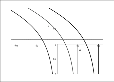
Figure 1: Solutions of Eq.(43)for different particle spin values. The horizontal straight line is $y={a_{0}}^{-1/2}$. The curves are $y=-2^{-1/2}\zeta[1/2,(1+s)/2+1/2a]$ and from left to right $s=-1,0,1$. The parameter $W=E^{\prime}/E_{0}$ is also shown.

It is obvious that the approximate solutions of (46) are quite near the intersections of the graphs of left-hand side of Eq.(43) (the straight line in Fig. 1) and of the right-hand sides of Eq.(43) (the curves in Fig. 1). We emphasize that the dependence of energy level shifts on the particle spin does not disappear in the strong-field limit. Moreover, the continuous spectrum boundaries are shifted in the cases $s=0$ and $s=1$. Hence, the perturbative displacements of the binding-energy levels (as in the weak-field limit) are at the same distances from the continuous spectrum boundaries in all cases.

We now consider spin interactions in the two-dimensional case. According to our approach, we can write

$$\ln\left(\frac{E}{E_{0}}\right)=\int\limits_{0}^{\infty}\frac{e^{-x}}{x}\left(\frac{axe^{-sax}}{{\rm sinh}(ax)}-1\right)dx,$$ (47)

where the particle spin direction, as before, is represented by $s=\pm 1$. In the weak-field limit, we obtain

$$\frac{E}{E_{0}}=1-\frac{s}{2}\frac{\hbar\omega}{E_{0}}-\frac{1}{24}\left(\frac{\hbar\omega}{E_{0}}\right)^{2}$$ (48)

from Eq.(47). To consider the strong-field limit, we must calculate the integral in Eq.(47) for $s=\pm 1$ in analytic form

$$\int\limits_{0}^{\infty}\frac{e^{-x}}{x}\left(\frac{axe^{-sax}}{{\rm sinh}(ax)}-1\right)dx=-2a\frac{(1+s)}{2}-\ln(2a)-\Psi\left(\frac{1}{2a}\right).$$ (49)

We can then write the equations for energy displacements for $\hbar\omega>E_{0}$ as

$$\ln\left(\frac{E}{E_{0}}\right)=2a\frac{(1-s)}{2}-\ln(2a)+C-\frac{\pi^{2}}{12a}.$$ (50)

For the case $s=-1$ in the strong-field limit ($\ln\frac{\hbar\omega}{E_{0}}>>1$) we immediately obtain

$$E^{\prime}=-\hbar\omega\left(\frac{1}{\ln\frac{\hbar\omega}{E_{0}}}+\frac{C}{\ln\frac{\hbar\omega}{E_{0}}}\right)$$ (51)

from Eq.(47).

For the opposite spin orientation ($s=1$) in Eq.(49), we must first use the recurrent relation for $\Psi(p)$,

$$\frac{1}{x}+\Psi(x)=\Psi(1+x).$$ (52)

Using the asymptotic expansion for $\Psi(p)$ (see (29)), then obtain

$$E^{\prime}=\hbar\omega\left(1-\frac{1}{\ln\frac{\hbar\omega}{E_{0}}}-\frac{C}{(\ln\frac{\hbar\omega}{E_{0}})^{2}}\right).$$ (53)

The dependence on the spin parameters can be interpreted as in three-dimensional model. We can write this equation in the form

$$\ln\left(\frac{\hbar\omega}{E_{0}}\right)=-\psi\left(\frac{1+s}{2}+\frac{1}{2a}\right).$$ (54)

In Fig.2, we show graphs of the solutions of Eq.(54) for different particle spin values with $E_{0}=10^{-3}eV$ and $\hbar\omega=100E_{0}$. The main difference from the three-dimensional model is that the perturbative binding-energy levels converge to the continuous spectrum boundaries in a superstrong magnetic field in this case.

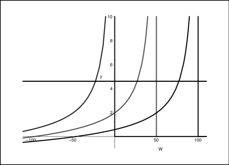
Figure 2: Solutions of Eq.(54)for different particle spin values. The horizontal straight line is $y=\ln{\hbar\omega/E_{0}}$. The curves are $y=-\Psi[(1+s)/2+1/2a]$ and from left to right $s=-1,0,1$. The parameter $W=E^{\prime}/E_{0}$ also shown.

4 The binding energy of spin-$0$ and spin-$1/2$ particles in the presence of the both weak and strong magnetic fields

We have shown that the effect of a magnetic field on localized electron states leads to equations for the binding energy of spin-$0$ and spin-$1/2$ particles. In the weak-field limit ($\hbar\omega\ll E_{0}$), the energy displacements of scalar and spinor particles are described by the expressions

$$\left.\begin{array}[]{rcl}s=0\,\,\,\,\,\,\frac{\hbar\omega}{2E_{0}}&+&\frac{E}{E_{0}}\\ s=1\,\,\,\,\,\,\,\,\frac{\hbar\omega}{E_{0}}&+&\frac{E}{E_{0}}\\ s=-1&{}\hfil&\frac{E}{E_{0}}\\ \end{array}\right\}=1+\frac{\hbar\omega}{2E_{0}}-\frac{\hbar^{2}\omega^{2}}{48{E_{0}}^{2}}.$$ (58)

in the three-dimensional case and

$$\left.\begin{array}[]{rcl}s=0\,\,\,\,\,\,\frac{\hbar\omega}{2E_{0}}&+&\frac{E}{E_{0}}\\ s=1\,\,\,\,\,\,\,\,\frac{\hbar\omega}{E_{0}}&+&\frac{E}{E_{0}}\\ s=-1&{}\hfil&\frac{E}{E_{0}}\\ \end{array}\right\}=1+\frac{\hbar\omega}{2E_{0}}-\frac{\hbar^{2}\omega^{2}}{24{E_{0}}^{2}}$$ (62)

in the two-dimensional case. From Eq.(58) and Eq.(62) we can also obtain

$$s=0:\,\,\,\,\,\,\,\,\,\,\,\,\,\,\,E=E_{0}-\frac{\hbar^{2}\omega^{2}}{24\delta{E_{0}}},$$

$$s=1:\,\,\,\,\,\,\,\,\,E=E_{0}-\frac{\hbar\omega}{2}-\frac{\hbar^{2}\omega^{2}}{24\delta{E_{0}}},$$

$$s=-1:\,\,\,\,\,\,\,E=E_{0}+\frac{\hbar\omega}{2}-\frac{\hbar^{2}\omega^{2}}{24\delta{E_{0}}},$$ (63)

where $\delta=2$ and $\delta=1$ in the three-dimensional and in the two-dimensional cases correspondingly.

The dependence on the particle spin does not disappear in the strong-field limit ($\hbar\omega\gg E_{0}$). In three-dimensional case, the perturbative energy levels approach specific spectral values determined by the magnetic field intensity. For different particle spin values, the displacements of the binding-energy levels as before [see Eq.(58)and Eq.(62)] are at identical distances from the continuous spectrum boundaries and can be represented in the form

$$\left.\begin{array}[]{rcl}s=0\,\,\,\,\,\,\,\,\,\frac{\hbar\omega}{2}&-&E^{\prime}\\ s=1\,\,\,\,\,\,\,\,\,\hbar\omega&-&E^{\prime}\\ s=-1&{-}&E^{\prime}\\ \end{array}\right\}=\hbar\omega\left(0.295+0.452\sqrt{\frac{E_{0}}{\hbar\omega}}+0.367\frac{E_{0}}{\hbar\omega}\right).$$ (67)

Removing the braces in Eq.(67), we find

$$s=0:\,\,\,\,\,\,\,\,E^{\prime}=0.205\hbar\omega-0.452\sqrt{E_{0}\hbar\omega}-0.367E_{0},$$

$$s=1:\,\,\,\,\,\,\,\,\,E^{\prime}=0.705\hbar\omega-0.452\sqrt{E_{0}\hbar\omega}-0.367E_{0},$$

$$s=-1:\,\,\,\,\,\,\,\,\,E^{\prime}=-0.295\hbar\omega-0.452\sqrt{E_{0}\hbar\omega}-0.367E_{0}.$$ (68)

In particular, from Eq.(68) one can immediately see that the value of the binding energy level is positive both in the case of a spinless particles ($s=0$) and in the case where the electron spin in oriented along the magnetic field direction ($s=1$), but it remains negative in the case where the electron spin is oriented against the magnetic field direction ($s=-1$).

It can be easily seen that the dependence on the spin parameters in the two-dimensional case can be written analogously,

$$\left.\begin{array}[]{rcl}s=0\,\,\,\,\,\,\,\,\,\frac{\hbar\omega}{2}&-&E^{\prime}\\ s=1\,\,\,\,\,\,\,\,\,\hbar\omega&-&E^{\prime}\\ s=-1&{-}&E^{\prime}\\ \end{array}\right\}=\frac{\hbar\omega}{\ln\frac{\hbar\omega}{E_{0}}}+\frac{C\,\,\hbar\omega}{(\ln\frac{\hbar\omega}{E_{0}})^{2}},$$ (72)

and without braces we have

$$s=0:\,\,\,\,\,\,\,\,E^{\prime}=\frac{\hbar\omega}{2}-\frac{\hbar\omega}{\ln\left(\frac{\hbar\omega}{E_{0}}\right)}-\frac{C\,\,\hbar\omega}{{\ln}^{2}\left(\frac{\hbar\omega}{E_{0}}\right)},$$

$$s=1:\,\,\,\,\,\,\,\,\,E^{\prime}=\hbar\omega-\frac{\hbar\omega}{\ln\left(\frac{\hbar\omega}{E_{0}}\right)}-\frac{C\,\,\hbar\omega}{{\ln}^{2}\left(\frac{\hbar\omega}{E_{0}}\right)},$$

$$s=-1:\,\,\,\,\,\,\,\,\,E^{\prime}=-\frac{\hbar\omega}{\ln\left(\frac{\hbar\omega}{E_{0}}\right)}-\frac{C\,\,\hbar\omega}{{\ln}^{2}\left(\frac{\hbar\omega}{E_{0}}\right)}.$$ (73)

It can be seen from Eq.(72) and Eq.(73) that the energy levels in the basic terms are also independent on the particle energy in the absence of the magnetic field. The distinctive feature of this case is that the binding-energy levels for superstrong magnetic fields [when $\ln(\hbar\omega/E_{0})>>1$] directly approach the continuous spectrum boundaries for all considered spin values.

We have shown that the energy levels of a polarized electron under the action of a weak magnetic field for different particle spin values are shifted similarly in the three-dimensional and two-dimensional models. We have the line displacements as the levels themselves for $s=1$ and $s=-1$ and analogous shifts of the continuous spectrum boundaries of for $s=1$. We also have the same picture in the case of a spinless particle with the line shift of the continuous spectrum boundary. Clearly, in case of weak intensity, a magnetic field indeed plays a stabilizing role in the considered systems because the depth of the perturbative binding-energy levels from the continuous spectrum boundaries are shifted downward under the field action independently of the particle spin. But our results show a nonlinear dependence on the field intensity in the strong-field limit. Nevertheless, the continuous spectrum boundaries in the cases $s=0$ and $s=1$, as before, have a linear dependence on the field in this limit. In superstrong magnetic fields, the binding-energy levels can approach the continuous spectrum boundaries. The distinctions can be formulated as follows. In the three-dimensional model, there is a fixed depth of the energy levels from the continuous spectrum boundaries that is the same for all spin values. In the two-dimensional model, the energy levels in a superstrong magnetic field tend asymptotically to the continuous spectrum boundaries. But in both cases, the system instability increases in strong magnetic fields. This conclusion therefore disproves the opinion that a magnetic field always plays a stabilizing role in systems of bound particles.

5 The exact analytic solution of the Pauli equation for the attractive three-dimensional $\delta$-well and its asymptotic expressions

The Green’s function obtained in [37] is the solution of the Pauli equation with a $\delta$-source and can be represented as an integral over time [38], [29]. This integral determining the Green’s function admits a Wick rotation to the lower complex half-plane of the variable $t$ (see, e.g., [26]). This operation makes the integral purely real. As a result, the stationary Green’s function can be represented in the form

$$G_{\text{W}}(\vec{r},\vec{0})={} -i\biggl{(}\frac{m}{2\pi}\biggr{)}^{3/2}\frac{\omega_{{}_{\!\!H}}}{2}e^{-im\omega_{{}_{\!\!H}}xy/4}\times{}$$

$${}\times\int_{0}^{\infty}\frac{dt}{t^{1/2}}\operatorname{sinh}^{-1}\biggl{(}\frac{\omega_{{}_{\!\!H}}t}{2}\biggr{)}e^{S/\hbar}\begin{pmatrix}1/2+s\\[2.84526pt] 1/2-s\end{pmatrix},$$ (74)

where $m$ is the particle mass, $\omega_{{}_{\!\!H}}=eH/mc$ is the cyclotron frequency, $e$ is the absolute value of the particle charge, $H$ is the strength of the uniform magnetic field oriented along the $z$ axis, $s=\pm 1/2$ is the spin number, and the argument of the exponential in the integrand is in fact the classical action function

$$S=-\frac{mz^{2}}{2t}-\frac{1}{4}m\omega_{{}_{\!\!H}}\rho^{2}\operatorname{coth}\biggl{(}\frac{\omega_{{}_{\!\!H}}t}{2}\biggr{)}+(W-s\cdot\hbar\omega_{{}_{\!\!H}})t$$ (75)

(although the argument of the exponential formally contains the Planck constant, this dependence vanishes because of the shift in the energy of a bound spinning particle in a magnetic field [28]). In formulas (1) and (2), $x$, $y$, and $z$ are the Cartesian coordinates, $\rho^{2}=x^{2}+y^{2}$, and $W<0$ is the total energy of the bound particle. We note that (1), (2) is the ordinary propagator of a charged particle moving in a magnetic field and is continued to the range of negative energies.

We write the spatial part of the wave function in the form

$$\psi(\vec{r}\,)=\widetilde{N}e^{-im\omega_{{}_{\!\!H}}xy/4}\int_{0}^{\infty}\frac{dt}{t^{1/2}}\operatorname{sinh}^{-1}\biggl{(}\frac{\omega_{{}_{\!\!H}}t}{2}\biggr{)}e^{S/\hbar},$$ (76)

where $\widetilde{N}$ is the normalizing coefficient. We pass to more natural variables using characteristic scales of the problem. As an energy scale, we take $|W_{0}|$, which is the absolute value of the particle binding energy in the absence of a magnetic field. We let $w=W/|W_{0}|$ denote the dimensionless binding energy in such units. It is equal to $-1$ in the absence of the external field. Of course, $w$ depends on both the external field $H$ and the spin direction in the general case [28]. It is convenient to measure the magnetic field in the dimensionless units $h=\hbar\omega_{{}_{\!\!H}}/|W_{0}|$. The de Broglie wavelength $l_{0}=\hbar(2m|W_{0}|)^{-1/2}$ of the particle for the zero magnetic field can serve as a natural coordinate scale, and the quantity $t_{0}=\hbar|W_{0}|^{-1}$ can serve as a time scale. Using such units for the spatial part of the wave function, we obtain

$$\psi(\vec{r}\,)=Ne^{-ih\tilde{x}\tilde{y}/4}\int_{0}^{\infty}\frac{d\tau}{\tau^{1/2}}\frac{\exp\big{[}-{\tilde{z}}^{2}/(4\tau)-h{\tilde{\rho}}^{2}\operatorname{coth}(h\tau/2)/8-\widetilde{w}\tau\big{]}}{1-e^{-h\tau}},$$ (77)

where $N$ is the normalizing coefficient in the new variables and $\tilde{x}$, $\tilde{y}$, $\tilde{z}$, and $\tau$ are the dimensionless coordinates and time. The analogy between the integrand in (4) and the classical Planck formula for the black-body emission spectrum is interesting. The quantizing character of the magnetic field (as the quantum character of radiation) is not manifested until the exponent factor $h\tau$ in the denominator in the right-hand side of (4) is sufficiently small. We also call attention to the phase factor $e^{-ih\tilde{x}\tilde{y}/4}$, whose presence explicitly demonstrates the existence of the orbital probability current.

To calculate the normalizing coefficient in (4), we must evaluate several integrals. The integrals over the coordinates are assumed to be purely Gaussian, and the integral over time can be reduced to the generalized Riemann zeta function $\zeta(3/2,\varepsilon)$ by a simple change of variables. As a result, we obtain

$$N=\frac{h^{5/4}}{2\pi l_{0}^{3/2}}\zeta^{-1/2}\biggl{(}\frac{3}{2},\frac{\widetilde{w}}{h}\biggr{)},$$ (78)

where $\widetilde{w}=w_{\mathrm{sh}}-w$ is the absolute value of the so-called effective energy of the particle. The parameter $\widetilde{w}$ appears because the lower edge of the continuum, together with the bound states $w$, is shifted in the magnetic field. Consequently, the binding effective energies are now measured from new boundaries determined by the expression $w_{\mathrm{sh}}=(s+1/2)h$ [28]. It also follows directly from this relation that the shift $w_{\mathrm{sh}}$ in the continuum depends explicitly on both the magnetic field and the particle spin orientation. But it was shown in [28] using weak ($h\ll 1$) and strong ($h\gg 1$) fields as examples that $\widetilde{w}$ is independent of the spin.

It is easy to see that the integral in (4) can be related to Laplace-type integrals [39], [40]. The relevant integration domain is determined by a neighborhood of a single point of the exponential maximum. We consider the contribution of the saddle point to the integral in (4) written in the form

$$\int_{0}^{\infty}\frac{du}{u^{1/2}}\frac{e^{-hg(u)}}{1-e^{-u}},\qquad g(u)=\frac{{\tilde{z}}^{2}}{4u}+\frac{\tilde{\rho}^{2}}{8}\operatorname{coth}\biggl{(}\frac{u}{2}\biggr{)}+\frac{\widetilde{w}}{h^{2}}u.$$ (79)

Here, $u=h\tau$, and the saddle point is a root of the equation

$$Bu^{2}-A=\frac{u^{2}}{\sinh^{2}(u/2)},\qquad A=4{\tilde{z}}^{2}\tilde{\rho}^{-2},\qquad B=16\widetilde{w}\tilde{\rho}^{-2}h^{-2}.$$ (80)

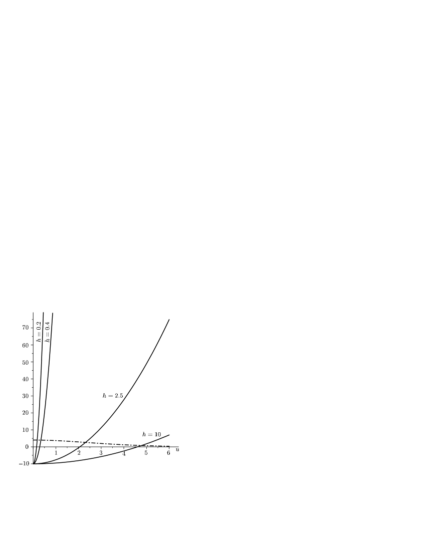
Figure 3: The solution of transcendental equation (7) in the plane $z=1.6$ for $\rho=1$. The solid curves correspond to the left-hand side of Eq. (7) for different values of the magnetic field, and the dot-dashed curve is the graph of the right-hand side of Eq. (7).

A graphic illustration of the search for the solution of this transcendental equation is shown in Fig. 3, which shows the family of parabolas corresponding to the left-hand side of Eq. (7) for different values of the parameter $h$ (the solid curves) and the graph of the function in the right-hand side of the equation (the dot-dashed curve). It is easy to verify that the parabola branch can intersect the monotonic function $u^{2}\sinh^{-2}(u/2)$ in various ranges of the integration parameter $u$. Hence, in the range $u\ll 1$, the right-hand side of the equation differs slightly from the constant, and the saddle point, which is the root of the quadratic equation in this case, is given by

$$u_{0}=\frac{h\sqrt{\tilde{\rho}^{2}+\tilde{z}^{2}}}{2\sqrt{\widetilde{w}}}.$$ (81)

In the other limit case $u\gg 1$, the right-hand side of Eq. (7) almost vanishes, and for the saddle point, we have

$$u_{0}=\frac{h\tilde{z}}{2\sqrt{\widetilde{w}}}.$$ (82)

Finally, for the intermediate range, the solution of Eq. (7) can be written in the approximate form

$$u_{0}\approx\biggl{[}\frac{\tilde{z}^{2}h^{2}}{8\widetilde{w}}-6+6\biggl{[}1+\frac{\tilde{z}^{2}h^{2}}{24\widetilde{w}}+\frac{\tilde{\rho}^{2}h^{2}}{12\widetilde{w}}+\frac{\tilde{z}^{4}h^{4}}{2304\widetilde{w}^{2}}\biggr{]}^{1/2}\biggr{]}^{1/2}.$$ (83)

It is easy to see that this solution in the limits of weak ($h\ll 1$) and strong ($h\gg 1$) fields respectively transforms into (8) and (9). In this case, the evaluation of integral (6) obtained by the saddle point approximation is written as

$$I(\tilde{z},\tilde{\rho})\approx 2\sqrt{\frac{\pi}{h}}\biggl{[}\frac{4\tilde{z}^{2}}{u_{0}^{2}}\sinh^{2}\biggl{(}\frac{u_{0}}{2}\biggr{)}+\frac{\tilde{\rho}^{2}u_{0}}{2}\operatorname{coth}\biggl{(}\frac{u_{0}}{2}\biggr{)}\biggr{]}^{-1/2}e^{(u_{0}/2)-hg(u_{0})}.$$ (84)

We now turn to studying the wave function in the limits of weak and strong fields. We see in what follows that these concepts require some more accurate definitions in the problem under consideration. If $h\ll 1$ and if $\tilde{\rho}$ and $\tilde{z}$ are not very large, then solution (8) reduces to

$$u_{0}=\frac{h\tilde{r}}{2\sqrt{\widetilde{w}}}\ll 1,$$ (85)

where $\tilde{r}=\sqrt{\tilde{z}^{2}+\tilde{\rho}^{2}}$ is the dimensionless radial coordinate. In the limit under consideration, this expression in fact determines the spherical type of symmetry of the electron cloud.

As already stated in the introduction, the behavior of the bound energy level of a spinning particle located in a $\delta$-well in the magnetic field was studied in [28]. It is important that the obtained solution has stable asymptotic expressions with respect to the spin variable in the limits of weak and strong fields, i.e., the effective energy characteristic $\widetilde{w}$ is independent of the spin in both cases. Although the computational technique used in [28] differs slightly from techniques used for scalar particles in the previous papers [15], [32], the results obtained in the limits of weak and strong fields in [28] agree completely. In particular, according to [28],we have $\widetilde{w}\approx 1+h/2$ for small magnetic fields, whence it can be directly seen that there is no dependence of $\widetilde{w}$ on the particle spin.

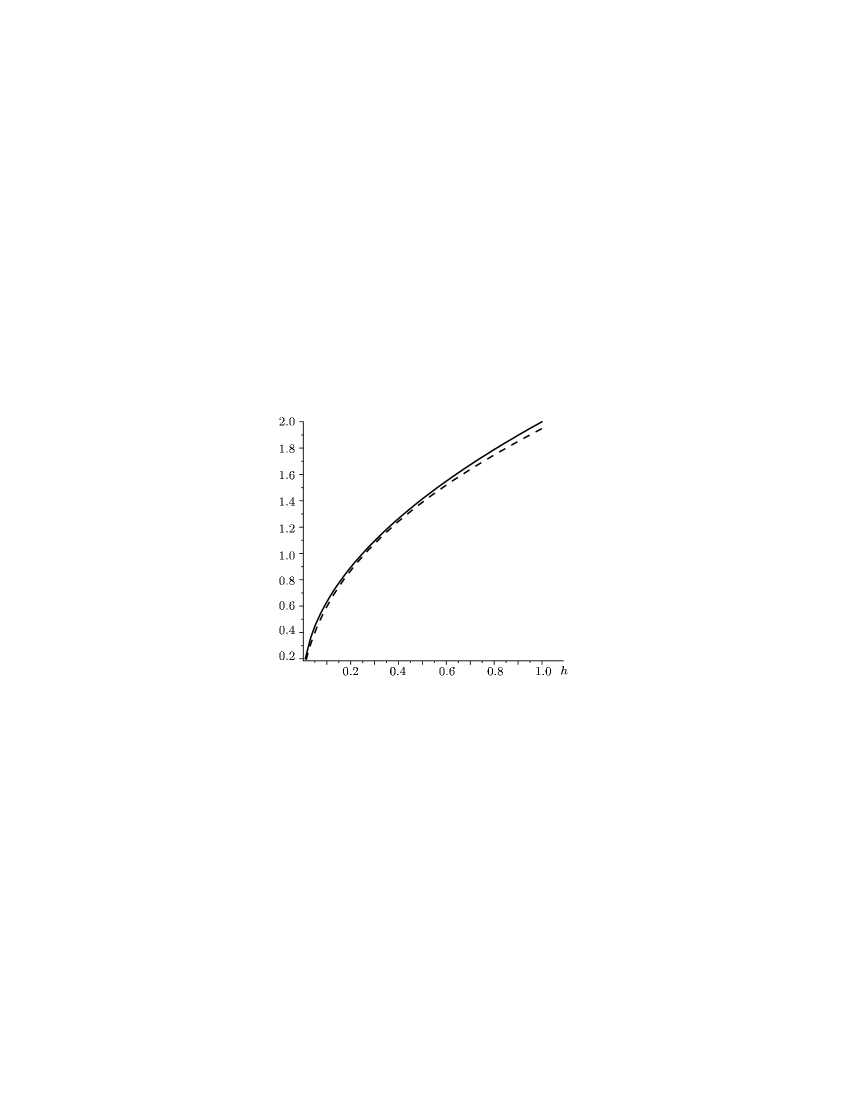
Figure 4: The exact dependence of the function $\zeta(3/2,\widetilde{w}/h)$ on the magnetic field $h$ (the dashed curve) and the dependence determined by the right-hand side of formula (13) (the solid curve).

Taking the foregoing into account, we use the estimate for the zeta function

$$\zeta\biggl{(}\frac{3}{2},\frac{\widetilde{w}}{h}\biggr{)}\sim 2h^{1/2},$$ (86)

which is applicable in the range $h\leq 1$. In particular, the graphs shown in Fig. 4 demonstrate that such an asymptotic expression is valid. Therefore, for the range under consideration $h<1$ (and not very far from the $\delta$-well), we obtain the expression

$$\psi(\vec{r}\,)\approx N\frac{2\sqrt{\pi}}{h\tilde{r}}\exp\biggl{(}-\frac{i}{4}h\tilde{x}\tilde{y}-\tilde{r}\biggr{)}$$ (87)

for the spatial part of the wave function.

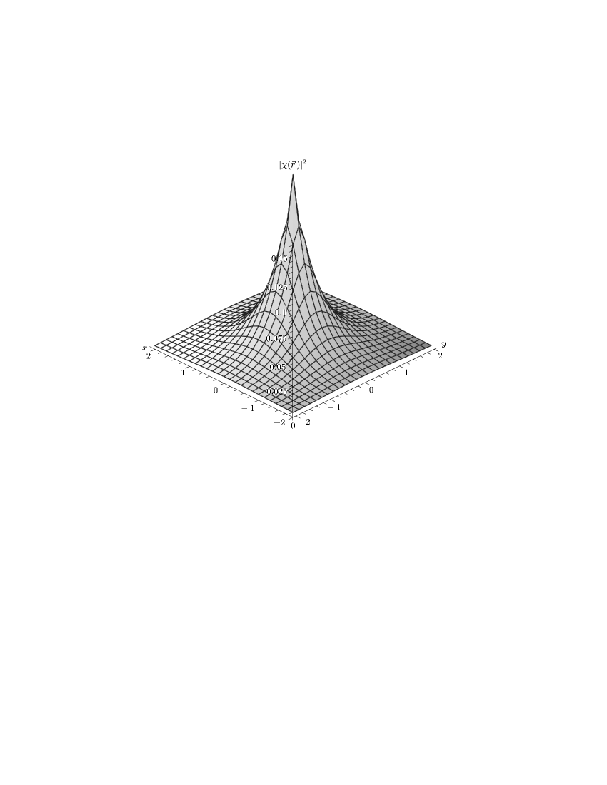
Figure 5: The dependence of the dimensionless squared function $|\chi(\vec{r}\,)|^{2}$ on the transverse ($x$) and longitudinal ($z$) coordinates for fields $h\leq 1$.

To represent the results graphically, it is convenient to use the function $\chi(\vec{r}\,)=r\psi(\vec{r}\,)$ having no singularities at zero and determining the spatial distribution of the probability density of the electron cloud in the spherical system of coordinates:

$$dW\sim 2\pi|\chi({\vec{r}}\,)|^{2}\sin(\theta)\,d\theta\,dr.$$

Figure 5 shows the graph of $|\chi(\vec{r}\,)|^{2}$. In this case, the de Broglie wavelength is assumed to be unity. We stress that this estimate for the wave function was obtained in the vicinity of the $\delta$-well in the weak field limit. But we note that the field of the order of several tenths of the interatomic field is not weak in the ordinary sense.

Far from the $\delta$-well, even in the weak field approximation, the case changes cardinally. For $h\tilde{z}\gg 1$, from formula (10), we have

$$u_{0}=\frac{h\tilde{z}}{2\sqrt{\widetilde{w}}}\gg 1$$ (88)

for the saddle point. As a result, the asymptotic expression for the spatial part of the wave function becomes

$$\psi(\vec{r}\,)\approx N\sqrt{\frac{\pi}{1+h/2}}\exp\biggl{(}-\frac{i}{4}h\tilde{x}\tilde{y}-\frac{h\tilde{\rho}^{2}}{8}-\tilde{z}\sqrt{1+\frac{h}{2}}\biggr{)}.$$ (89)

This expression is important for a qualitative analysis. The solution has an axial symmetry in this range. It is clear that the value of the field determines the range where the spherical symmetry typical of the bound s state transforms into the axial symmetry inherent in the wave functions of particles in a purely magnetic field. In addition, it can be seen that at large distances from the $\delta$-well even in the weak-field case, only the ground level of the effective energy makes the main contribution, i.e., the level located at the smallest distance from the continuum edge ($1+h/2$ in our adopted units). This agrees completely with the conclusions in [32], [28]. In the case where the processes with free particles in an external magnetic field are considered, it is usually assumed that the weak field does not always exhibit its quantizing character, yielding only small corrections to the cross sections of the corresponding processes. In contrast, it is traditionally assumed that only several minimum-energy levels contribute in the strong-field case [26].

In contrast to this, in the case of a bound state, any arbitrarily weak field behaves as a strong field at large distances from the center. In particular, it follows from (16) that the magnetic field compresses the electron cloud not only in the direction transverse to the field (which can be expected) but also along the field. But if the shift in the ground level of the effective energy in the magnetic field is neglected, i.e., if it is assumed that $\widetilde{w}=1$, then such effects cannot be described. We note that under these simplifying assumptions, solution (16) agrees with the basic function used in [34].

For a strong field, the case is more complicated. The reason is obvious because the intermediate range in which the symmetry transforms from the spherical into the axial one in this case belongs to the range where the wave function differs significantly from zero. Using the results in [28] on determining the effective energy of the electron in strong fields ($h\gg 1$), $\widetilde{w}\approx 0.295h$, we consider a small neighborhood of the $\delta$-center. For $\tilde{r}\ll 1/\sqrt{h}$, the position of the saddle point is determined by expression (12). For the wave function, using relations (4) and (11), we obtain an analogue of expression (14) but with a different effective energy:

$$\psi(\vec{r}\,)\approx N\frac{2\sqrt{\pi}}{h\tilde{r}}\exp\biggl{(}-\frac{i}{4}h\tilde{x}\tilde{y}-\tilde{r}\sqrt{0.295h}\biggr{)}.$$ (90)

Therefore, supplementing our conclusions on the behavior of the function at large distances in a weak field, we note that any arbitrarily strong field behaves as a weak one in the direct vicinity of the attractive $\delta$-center. The reason is that the depth of the $\delta$-well is much greater than any finite shift in the energy level in the magnetic field. The equation for the bound level energy $w(h)$ follows precisely from the fact that the character of this asymptotic expression is independent of the external magnetic field [15], [32], [28].

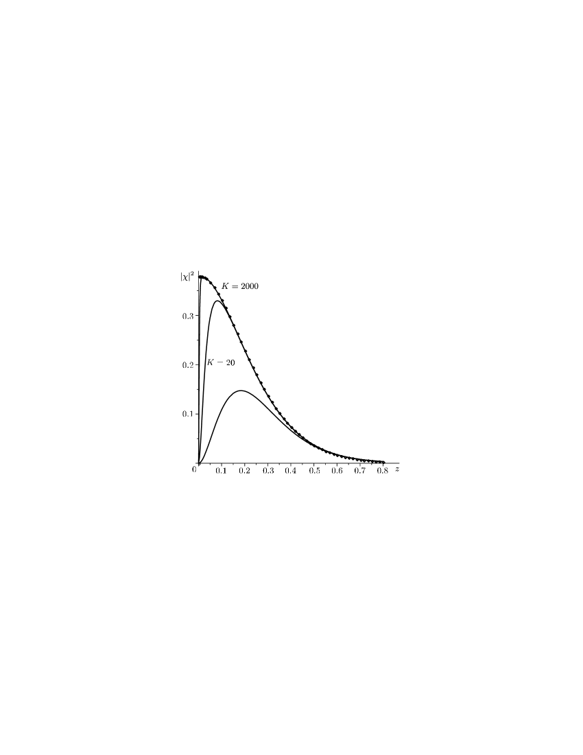
Figure 6: The dependence of $|\chi(\vec{r}\,)|^{2}$ on $z$ on the axis $\rho=0$ for the field $h=100$. The points correspond to the calculation using formula (4), and the solid curves (successively from the bottom up) determine the strong field approximations: the contribution of the ground level (18) and the contributions for $K=20$ and $K=2000$ calculated using formula (20).

The wave function becomes axially symmetric in the strong field at distances $\tilde{z}\gg 1/\sqrt{h}$. For $h\gg 1$ and fixed $\tilde{\rho}\neq 0$ and $\tilde{z}\neq 0$, we obtain formula (15). For the wave function, from relations (4) and (11), we obtain an analogue of formula (16) in the case of strong fields:

$$\psi(\vec{r}\,)\approx N\sqrt{\frac{\pi}{0.295h}}\exp\biggl{(}-\frac{i}{4}h\tilde{x}\tilde{y}-\frac{h\tilde{\rho}^{2}}{8}-\tilde{z}\sqrt{0.295h}\biggr{)}.$$ (91)

It is easy to see that also in this case, only the ground level of the effective energy contributes.

Spherically symmetric estimate (12) and axially symmetric estimate (15) of the maximum point agree in a neighborhood of the straight line $\tilde{\rho}=0$. It is interesting that the dependence of the bound level energy on the magnetic field was first obtained in [32], where the limit transition in the expression for the wave function was used precisely along this line. Therefore, to extend the applicability range of the obtained expression (18) to the range of small $z$, we can expand the denominator in initial formula (4) into a geometric series in terms of partial effective levels,

$${\widetilde{w}}_{k}=\widetilde{w}+kh,\quad k=0,1,2,\dots,$$ (92)

replacing the Landau levels in a purely magnetic field [20], and use estimate (18) for each term. The wave function in this case becomes

$$\psi(\vec{r}\,)\approx N\sqrt{\pi}\exp\biggl{(}-\frac{i}{4}h\tilde{x}\tilde{y}-\frac{h\tilde{\rho}^{2}}{8}\biggr{)}\sum_{k=0}^{K}\frac{e^{-\tilde{z}\sqrt{(0.295+k)h}}}{\sqrt{(0.295+k)h}}.$$ (93)

It is easy to verify that if the maximum number $K$ of levels taken into account increases, then the applicability range for the obtained formula can be extended to arbitrarily small values of the coordinate $z$.

In Fig. 6, the squared function $|\chi|^{2}$ calculated using exact formula (4) is compared with asymptotic expressions (18) and (20) for the field $h=100$ and the axis $\rho=0$. The larger the parameter $\sqrt{h}z$ is, the better the series in solution (20) converges (and the first term of series (18) consequently approaches the exact solution). This turns out to be important because the probability current is maximum in this range.

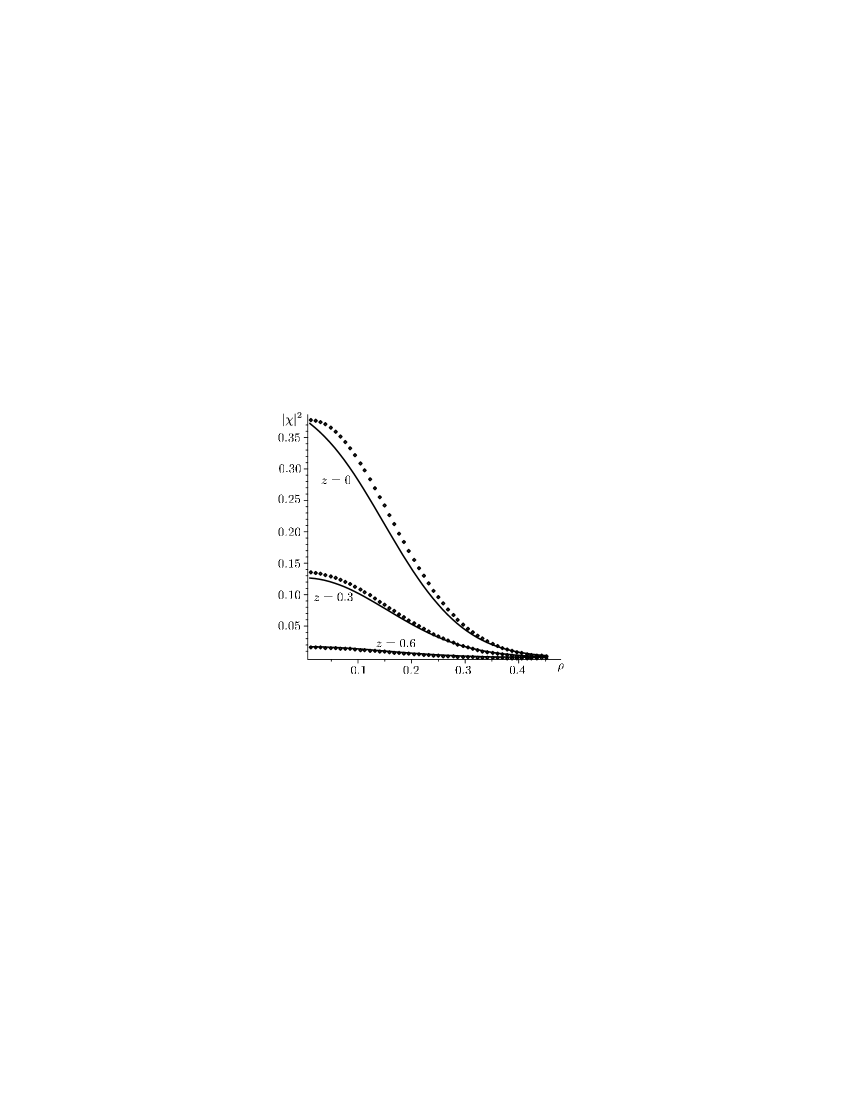
Figure 7: The dependence of $|\chi|^{2}$ on $\rho$ for the field $h=100$ and different $z$. The points correspond to the calculation using exact formula (4), and the solid curves correspond to strong field approximations using formulas (10) and (11).

Figure 7 shows the comparison of the expressions for $|\chi|^{2}$ in the case of three different values of $z$ ($z=0,0.3,0.6$) and the strong field $h=100$ calculated using exact formula (4) and approximate formula (11) with (10) taken into account.

We briefly summarize the results in this section. The solution of the Pauli equation is spherically symmetric for a weak magnetic field in the entire relevant range of coordinates. It is in fact determined only by the character of the singularity in the $\delta$-well; all effective partial levels $\widetilde{w}_{k}$ contribute to the formation of this singularity (see formula (19)). The quantizing character of the magnetic field (i.e., the tangibility of the contribution of individual energy levels) is manifested only far from the center in the region where the wave function is exponentially suppressed. For the strong field, the character of the solution symmetry changes in the relevant range of coordinates. The relative contribution of individual levels for a fixed field strength is mainly determined by the longitudinal coordinate (in the magnetic field direction), although the electron cloud is mainly compressed by the magnetic field in the transverse direction.

6 Probability currents of a particle bound by the $\delta$-potential in a magnetic field

The general expression for the nonrelativistic probability current of the spinor was given in the classic monograph [20]. Using the usual tensor notation, we represent this current $J_{k}$ in the form

$$J_{k}=-i\frac{\hbar}{2m}[(\nabla_{k}\psi^{*}_{\alpha})\psi_{\alpha}-\psi^{*}_{\alpha}\nabla_{k}\psi_{\alpha}]+\frac{e}{mc}A_{k}\psi^{*}_{\alpha}\psi_{\alpha}-\frac{\mu c}{e|s|}\varepsilon_{kpq}\nabla_{p}(\psi^{*}_{\alpha}\widehat{\sigma}^{q}_{\alpha\beta}\psi_{\beta}),$$ (94)

where $k=1,2,3$ are the spatial coordinate indices, $\alpha=1,2$ are the spin indices, $\nabla_{k}$ is the usual gradient operator, $A_{k}$ is the vector potential of the external magnetic field, $\mu$ is the electron magnetic moment, $\varepsilon_{kpq}$ is the unit totally antisymmetric tensor, and $\widehat{\sigma}^{q}_{\alpha\beta}$ are the binary sigma matrices. The complete normalized solution of the Pauli equation can be represented in the form

$$\psi_{\alpha}(\vec{r}\,)=\psi(\vec{r}\,)\begin{pmatrix}1/2+s\\[2.84526pt] 1/2-s\end{pmatrix},$$

where the spatial part $\psi(\vec{r}\,)$ is given by (4). The first and second terms in (21) determine the gradient (orbital) current, and the last term corresponds to the spin current.

Contracting spin indices with the explicit form of the sigma matrices taken into account, we obtain the spatial components of the total probability current

$$J_{x}=-i\frac{\hbar}{2m}\biggl{(}\frac{\partial\psi^{*}}{\partial x}\psi-\psi^{*}\frac{\partial\psi}{\partial x}\biggr{)}+\frac{e}{mc}A_{x}\psi^{*}\psi-\frac{\mu c}{e}\frac{s}{|s|}\frac{\partial}{\partial y}(\psi^{*}\psi),$$

$$J_{y}=-i\frac{\hbar}{2m}\biggl{(}\frac{\partial\psi^{*}}{\partial y}\psi-\psi^{*}\frac{\partial\psi}{\partial y}\biggr{)}+\frac{e}{mc}A_{y}\psi^{*}\psi+\frac{\mu c}{e}\frac{s}{|s|}\frac{\partial}{\partial x}(\psi^{*}\psi),$$

$$J_{z}=-i\frac{\hbar}{2m}\biggl{(}\frac{\partial\psi^{*}}{\partial z}\psi-\psi^{*}\frac{\partial\psi}{\partial z}\biggr{)}+\frac{e}{mc}A_{z}\psi^{*}\psi.$$

We must fix the gauge of the vector potential for further calculations. Choosing it as $A_{x}=-Hy$ and $A_{y}=A_{z}=0$ and passing to the dimensionless coordinates, we obtain

$$\vec{J}=\biggl{(}\frac{|W_{0}|}{2m}\biggr{)}^{1/2}\frac{h}{2}\psi^{*}\psi(\vec{j}\tilde{x}-\vec{i}\tilde{y})+\frac{(2m|W_{0}|)^{1/2}}{2\hbar}\frac{\mu c}{e}\frac{s}{|s|}\psi^{*}\widetilde{\psi}(\vec{j}\tilde{x}-\vec{i}\tilde{y}),$$ (95)

where $\vec{i}$ and $\vec{j}$ are the unit vectors of the Cartesian system and the function $\widetilde{\psi}(\vec{r}\,)$ has the form

$$\widetilde{\psi}(\vec{r}\,)=Ne^{-ih\tilde{x}\tilde{y}/4}\int_{0}^{\infty}\frac{d\tau}{\tau^{1/2}}\frac{1+e^{-h\tau}}{[1-e^{-h\tau}]^{2}}\exp\biggl{[}-\frac{\tilde{z}^{2}}{4\tau}-\frac{h}{8}\tilde{\rho}^{2}\operatorname{coth}\biggl{(}\frac{h\tau}{2}\biggr{)}-\widetilde{w}\tau\biggr{]}.$$

Assuming that the electron magnetic moment is equal to the Bohr magneton, we obtain

$$\vec{J}=\biggl{(}\frac{|W_{0}|}{2m}\biggr{)}^{1/2}\frac{h}{2}\psi^{*}(\psi+2s\widetilde{\psi})(\vec{j}\tilde{x}-\vec{i}\tilde{y}).$$ (96)

Using exact expression (4) for the spatial part of the wave function, we obtain the formula for the probability current in the case of an arbitrary spin orientation and field strength:

$${\vec{J}}={} Mh^{7/2}\zeta^{-1}\biggl{(}\frac{3}{2},\frac{\widetilde{w}}{h}\biggr{)}(\vec{j}\tilde{x}-\vec{i}\tilde{y})\times{}$$

$${}\times\int_{0}^{\infty}\frac{d\tau}{\tau^{1/2}}\frac{\exp\bigl{[}-\tilde{z}^{2}/(4\tau)-h\tilde{\rho}^{2}\operatorname{coth}(h\tau/2)/8-\widetilde{w}\tau\bigr{]}}{1-e^{-h\tau}}\times{}$$

$${}\times\int_{0}^{\infty}\frac{d\tau}{\tau^{1/2}}\frac{\exp[-\tilde{z}^{2}/(4\tau)-h\tilde{\rho}^{2}\operatorname{coth}(h\tau/2)/8-\widetilde{w}\tau]}{1-e^{-h\tau}}\times{}$$

$${}\times\biggl{[}1+2s\cdot\operatorname{coth}\biggl{(}\frac{h\tau}{2}\biggr{)}\biggr{]},$$ (97)

where $M=m|W_{0}|^{2}/4\pi^{2}\hbar^{3}$ is a dimension factor independent of the magnetic field.

We obtain the estimates for the current in the weak-field approximation. In this case, we have

$$\widetilde{\psi}(\vec{r}\,)\approx N\cdot\frac{8\sqrt{\pi}}{h^{2}\tilde{r}^{3}}(1+\tilde{r})\exp\biggl{(}-\frac{i}{4}h\tilde{x}\tilde{y}-\tilde{r}\biggr{)}.$$

Also taking (14) and (23) into account, we write the expression for the probability current in the weak magnetic field:

$$\vec{J}=M\zeta^{-1}\biggl{(}\frac{3}{2},\frac{1}{h}+\frac{1}{2}\biggr{)}\frac{4\pi h^{3/2}}{\tilde{r}^{2}}e^{-2\tilde{r}}\biggl{[}1+2s\cdot\frac{4(1+\tilde{r})}{h\tilde{r}^{2}}\biggr{]}(\vec{j}\tilde{x}-\vec{i}\tilde{y}).$$ (98)

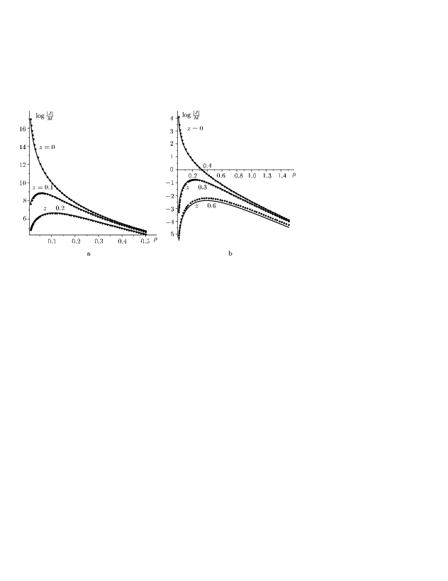
Figure 8: The dependencies of $\ln\big{(}|J|/M\big{)}$ on the transverse coordinate in the planes $z=\text{const}$ for the weak field $h=0.1$ in the cases of (a) the particle with spin directed opposite the field and (b) the scalar particle. The points correspond to the calculation using exact formula (24), and the solid curves correspond to weak-field approximation (25).

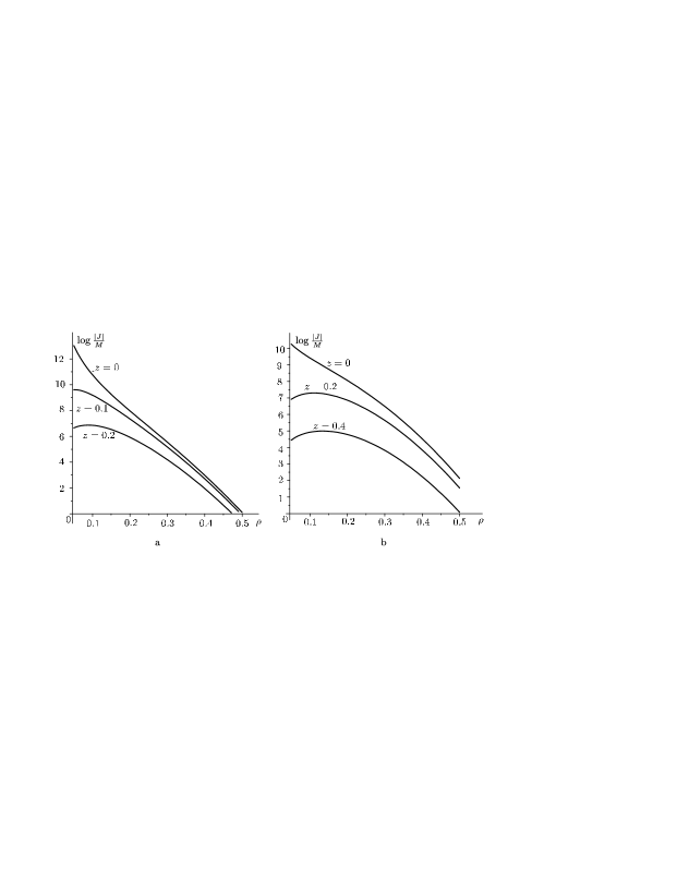
Figure 9: The dependencies of $\ln\big{(}|J|/M\big{)}$ on the transverse coordinate calculated using exact formula (24) in the planes $z=\text{const}$ for the strong field $h=100$ in the cases of (a) the particle with the spin directed opposite the field and (b) the scalar particle.

Figure 8a shows the dependencies of the logarithm of $|J|/M$ on the transverse coordinate $\rho$ in different planes $z=\text{const}$ for the field $h=0.1$; they are calculated using exact and approximate formulas (24) and (25) for $s=-1/2$, i.e., for the particle with the spin oriented opposite the field. In the case of the particle with the spin along the field, only the orientation of the vector $\vec{J}$ changes, i.e., the direction of the particle rotation changes. This occurs because the second term in (25) in the vicinity of the $\delta$-well turns out to be much greater than the first term. In other words, the orbital probability current in this case is negligibly small compared with the spin one. They become comparable only at a distance $\tilde{r}\sim 1/h$ from the center, where the current in the weak field ($h\ll 1$) is exponentially suppressed. This conclusion is confirmed by comparing Fig. 8a with Fig. 8b, where the same quantity $\ln\big{(}|J|/M\big{)}$ is constructed for the scalar particle. In this case, the spatial part of the wave function in the weak field (see formula (14)) is independent of the spin. The obtained result is quite expectable if we recall that in the case of a weak field, the $\delta$-well itself can bind a charged particle only if it is in the s state.

The dependencies of $\ln(|J|/M)$ on the transverse coordinate in the planes with different $z$ for the strong magnetic field $h=100$ demonstrating the spatial distribution of the probability currents are shown in Fig. 9a for the electron with the spin directed opposite the field and in Fig. 9b for the scalar particle. Exact formula (24) is used in the calculation.

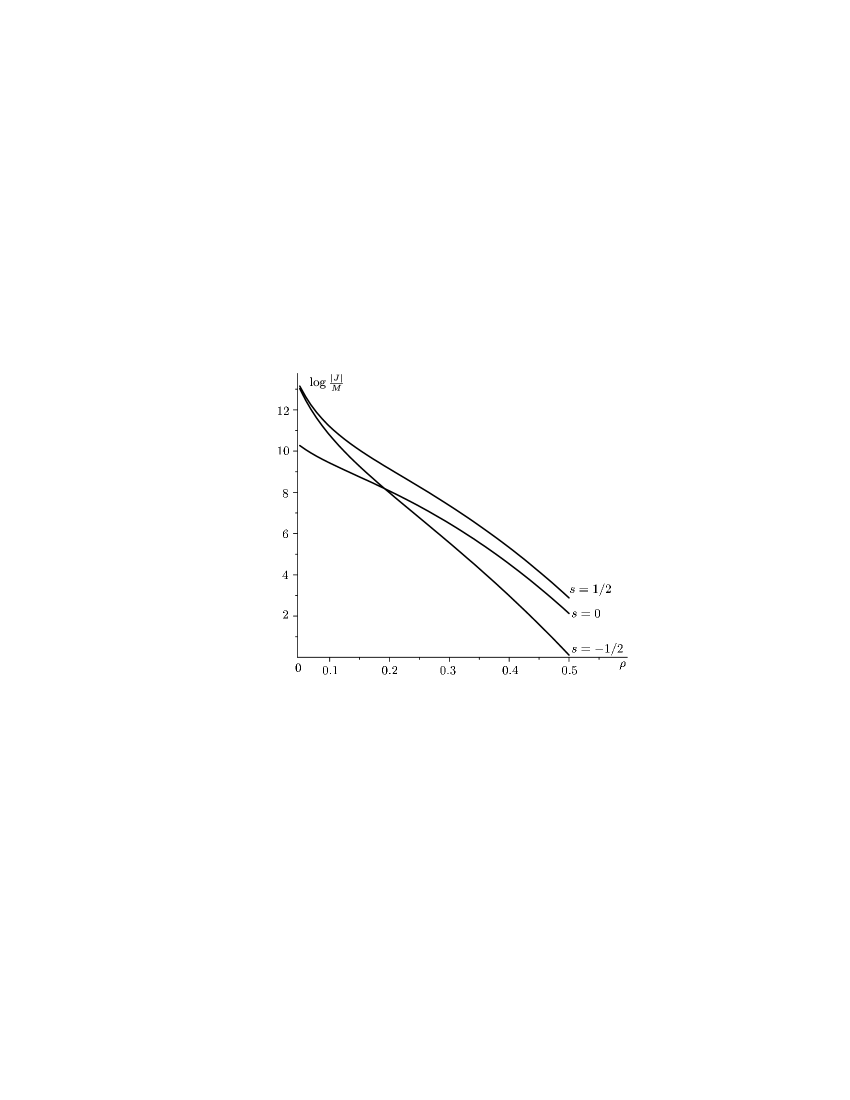
Figure 10: The dependence of $\ln\big{(}|J|/M\big{)}$ on the transverse coordinate obtained using exact formula (24) in the case of the plane $z=0$ and the strong field $h=100$ for different spin orientations (along the field and opposite the field) and the zero spin.

Figure 10 shows the comparison of the behavior of $\ln(|J|/M)$ for the scalar particle with that for the electron with its different spin orientations in the case of the strong field and the plane $z=0$. In particular, it can be seen from Fig. 8 that the orbital and spin currents in the strong field become comparable in the vicinity of the $\delta$-center. As should be expected, in the case of the electron with the spin oriented opposite the magnetic field, the current decreases more rapidly as the distance from the center increases, i.e., this particle motion is localized. The range where the orbital and spin currents turn out to be comparable is probably most interesting for studies.

Acknowledgments

This work was supported in part by the Program for Supporting Leading Scientific Schools (Grant Nos. NSh-8265.2010.1, G. A. K.) and the Russian Foundation for Basic Research (Grant No. 09-02-00725_a).

References

- [1]
- [2] Franz W. 1958, Z. Naturf. A. 13. 484
- [3] Keldysh L. V. 1958, Zh. Exsp. Teor. Fiz. 34. 1138 (Engl. transl. 1959, Sov. Phys. - JEPT. 34. 788)
- [4] Zel’dovich Ya. B. 1961, Zh. Exsp. Teor. Fiz. 39. 776 (Engl. transl. 1961, Sov. Phys. - JEPT 12. 542)
- [5] Demkov Yu. N. and Drukarev G. F. 1964, Zh. Exsp. Teor. Fiz. 47. 918 (Engl. transl. 1965, Sov. Phys. - JEPT 20. 614)
- [6] Demkov Yu. N. and Drukarev G. F. 1965, Zh. Exsp. Teor. Fiz. 49. 257 (Engl. transl. 1965, Sov. Phys. - JEPT 22. 182)
- [7] Keldysh L. V. 1964, Zh. Exsp. Teor. Fiz. 47. 1945 (Engl. transl. 1965, Sov. Phys. - JEPT 20. 1037)
- [8] Seraphin B. O. and Bottka N. 1965, Phys. Rev. 139. A560
- [9] Aspnes D. E. 1966, Phys. Rev. 147. 554
- [10] Ritus V. I. 1966, Zh. Exsp. Teor. Fiz. 51. 1544 (Engl. transl. 1967, Sov. Phys. - JEPT 25. 1027)
- [11] Drukarev G. F. and Monozon B. S. 1971, Zh. Exsp. Teor. Fiz. 61. 956 (Engl. transl. 1972, Sov. Phys. - JEPT 34. 509)
- [12] Nikishov A. I. 1972, Zh. Exsp. Teor. Fiz. 62. 562 (Engl. transl. 1972, Sov. Phys. - JEPT 35. 298)
- [13] Baz A. I, Zel’dovich Ya. B. and Perelomov A. M. 1971, Scattering, Reactions and Decays in Nonrelativistic Quantum Mechanics 2nd edn (Moscow: Nauka) (in Russian) (Engl. transl. - 1st edn, US Department of Commerce, Natural Technical Information Service, N69. 25848)
- [14] Zel’dovich Ya. B, Manakov N. L. and Rapoport L. P. 1975, Usp. Fiz. Nauk 117. 569 (Engl. transl. 1975, Sov. Phys.- Usp. 18. 920)
- [15] Popov V. S, Karnakov B. M. and Mur V. D. 1998, Zh. Exsp. Teor. Fiz. 113. 1579 (Engl. transl. 1998, Sov. Phys. - JEPT 86. 860)
- [16] Manakov N. L, Frolov M. V, Starace A. F. and Fabrikant I. I. 2000, J Phys B: At Mol Opt Phys 33. R141
- [17] Rodionov V. N, Kravtzova G. A. and Mandel A. M. 2002, Zh. Exsp. Teor. Fiz. Lett. 75. 435 (Engl. transl. 2002, Sov. Phys. - JEPT Letters 75. 363)
- [18] Rodionov V. N, Kravtzova G. A. and Mandel A. M. 2003, Zh. Exsp. Teor. Fiz. Lett. 78. 253 (Engl. transl. 2003, Sov. Phys. - JEPT Letters 78. 218)
- [19] Demkov Yu. N. and Ostrovsky V. N. 1988, Zero-Range Potentials and Their Applications in Atomic Physics (New York: Plenum)
- [20] L. D. Landau and E. M. Lifshits Theoretical Physics [in Russian], Vol. 3, Quantum Mechanics: Non-Relativistic Theory, Nauka, Moscow (1974); English transl.: 1992, Quantum Mechanics 4th edn (Oxford: Pergamon).
- [21] The Quantum Hall Effect, ed. by R. E. Prange and S. M. Girvin, 1990, Sprimger, New York.
- [22] F. Wilczec 1990, Fractional Statistic and Anyon Superconductivity, World Scientific, Singapore.
- [23] Chibirova F.Kh. Phys. Solid State, 2001, 43, p.1291.
- [24] A.M.J. Schakel. Phys. Rev. 1991, 43 1428.
- [25] A.Neagu and A.M.J. Schakel. Phys. Rev. 1993, 48 1785.
- [26] Ternov I.M., Khalilov V.R., Rodionov V.N., 1982, Interaction of Charged Particles with a Strong Electromagnetic Field, [in Russian], Moscow State Univ., Moscow.
- [27] V.R. Khalilov, Electrons in Strong Electromagnetic Fields (Gordon & Breach Sci.Pub., Amsterdam, 1996).
- [28] V. N. Rodionov, Phys. Rev. A, 75, 062111 (2007); arXiv:hep-ph/0702228 (2007).
- [29] V. N. Rodionov, G. A. Kravtsova and A. M. Mandel’ Teor. Mat. Fiz. 164. no.1, p.157 (2010) (Engl. transl.Theor. Math. Phys., 164, 960 (2010).
- [30] V. S. Popov, Phys. Uspekhi, 47, 855–885 (2004).
- [31] V. N. Rodionov, G. A. Kravtsova, and A. M. Mandel’, Dokl. Phys., 47, 725–727 (2002).
- [32] Yu. N. Demkov and G. F. Drukarev, Sov. Phys. JETP, 22, 479–484 (1966).
- [33] Kravtzova G. A., Rodionov V. N. and Mandel A. M. Ionization under the action of electromagnetic fields of complex configuration. in: Proc. of the Third Int. Sakharov Conf. on Physics, Moscow, 2002, ed. by V. N. Zaikin, M. A. Vasil’ev and A.M.Semikhatov, Nauchnyi Mir, Moscow, 2003, p.785.
- [34] Chibirova F.Kh., Khalilov V.R. Mod. Phys. Lett. A, 2005, 20., no. 9, p. 663.
- [35] Khalilov V.R., Chibirova F.Kh. Int. J. Mod.Phys., 2006, 21., p. 3171.
- [36] R. P. Feynman and A. R. Hibbs Quantum Mechanics and Path Integrals, Maidenhead, Berkshire, McGraw-Hill (1965).
- [37] V. N. Rodionov and A. M. Mandel, Moscow Univ. Phys. Bull., 56, 28–33 (2001).
- [38] G. A. Kravtsova, A. M. Mandel’, and V. N. Rodionov, Theor. Math. Phys., 145, 1539–1550 (2005).
- [39] M. V. Fedoryuk Asymptotics: Integrals and Series [in Russian], Nauka, Moscow (1987).
- [40] A. B. Migdal Qualitative Methods in Quantum Theory [in Russian], Nauka, Moscow (1975); English transl. (Lect. Notes and Reprint Ser., Vol. 48) W. A. Benjamin, London (1977).