Magnetic field control of intersubband polaritons in narrow-gap semiconductors

Abstract

We investigate theoretically the polariton coupling between the light confined in a planar cavity and the intersubband transitions of a two-dimensional electron gas confined in semiconductor quantum wells in the presence of a vertical magnetic field. We show that in heterostructures made of non-parabolic semiconductors, the polaritons do not fit a two-level problem, since the cavity photons couple to a non-degenerate ensemble of intersubband transitions. As a consequence, the stationary polariton eigenstates become very sensitive to the vertical magnetic field, which thus plays the role of an external parameter that controls the regime of light–matter interactions. At intermediate field strength we predict that the magneto-polaritons have energy dispersions ideally suited to parametric amplification.

I Introduction

Intersubband (ISB) polaritons are mixed states formed by the strong coupling of the light within a microcavity and the intersubband transitions of electrons confined in a semiconductor quantum well (QW) embedded in the cavity. Since the first experimental demonstration in 2003Dini et al. (2003) with a GaAs/AlGaAs multiple quantum well (MQW) structure, intense research efforts have been devoted to the study of ISB polaritons. With this kind of polaritons the light–matter coupling can reach very large valuesDupont et al. (2007); Anappara et al. (2007) becoming comparable to (or even larger than) the bare frequency of the cavity and of the ISB excitations. In this ultrastrong coupling regime, interesting quantum effects appear.Ciuti et al. (2005); De Liberato et al. (2007, 2009); Nataf and Ciuti (2010) Moreover, since the coupling strength is proportional to the square root of the number of electrons, it can be controlled by electrical gating.Anappara et al. (2005); Günter et al. (2009) Beside the observation of the strong coupling regime by means of reflectance spectroscopy as in the first experiments, and of photovoltaic measurements,Sapienza et al. (2007) also the electrical injection of cavity polaritons and their electroluminescence is being studied with considerable effort.Colombelli et al. (2005); Sapienza et al. (2008); Todorov et al. (2008); Jouy et al. (2010) Moreover, the coupling of the ISB transition with a surface plasmon supported by a metal grating has been demonstrated.Zanotto et al. (2010) In the effort of reaching larger light–matter couplings toward the ultrastrong coupling regime, other materials beside GaAs/AlGaAs have been considered, like for instance InAs/AlSb MQWs. Also the smaller effective mass of InAs with respect to GaAs ($m^{*}_{\text{InAs}}/m^{*}_{\text{GaAs}}=0.39$) implies a stronger coupling.Anappara et al. (2007) At zero magnetic field, the polaritons can be simply and effectively described by a two-level problem,Ciuti et al. (2005) where the first level is the cavity mode with energy $E_{\text{cav}}$, and the second level is the ISB transition with energy $E_{21}$ between the first (ground) and the second (excited) subband; the coupling is quantified by the Rabi frequency $\Omega_{R}$, where $2\hbar\Omega_{R}$ gives the splitting of the upper and lower polariton branches at the resonance $E_{\text{cav}}=E_{21}$.

When a magnetic field $B$ is applied along the QW growth axis $\hat{z}$, neither the energies nor the strength of the ISB–cavity coupling are altered; thus, a fortiori, the two-level description of the polariton levels remains valid, if we still focus on transitions between the Landau levels belonging to different subbands. A theoretical study on the possibility of obtaining ultrastrong magneto-polaritons couplings exploiting transitions between Landau levels in the same subband is reported in Ref. Hagenmüller et al., 2010. Actually, the aforementioned insensitivity to a vertical magnetic field is exact only for parabolic-band materials. It remains a very good approximation for GaAs-based heterostructures, since GaAs shows very little non-parabolicity. On the contrary, as we show below, in narrow-gap semiconductors like InAs or InSb, the band non-parabolicity effects cannot be disregarded in the calculation of the polaritonic states.

In this work, we demonstrate that in the non-parabolic case the ISB polaritons cannot be simply described in terms of two levels. Instead, the cavity photons couple to a non-degenerate ensemble of ISB transitions, giving rise to a complex evolution of the polariton dispersion for increasing $B$. We shall show that three different coupling regimes exist as a function of the intensity of the magnetic field. To this end, we consider a InAs/AlSb MQW heterostructure grown along the $\hat{z}$ axis. This choice is motivated by the experimental observation of ISB polaritons in this system,Anappara et al. (2007) as well by the significant band non-parabolicity of InAs. Band parameters and band offsets are taken from Ref. Vurgaftman et al., 2001. We consider a cavity with effective thickness $L_{z}$ so that for the lowest mode $k_{z}=\pi/L_{z}$ holds. The photon energy is given by $E_{\text{cav}}=(\hbar c/\sqrt{\varepsilon_{\infty}})\sqrt{k_{\parallel}^{2}+k_{z}^{2}}$, where $k_{\parallel}$ is the in-plane $\mathbf{k}$ vector and $\varepsilon_{\infty}$ is the dielectric constant of the material embedded in the cavity. Due to the usual ISB selection rules, we consider only light which is TM polarized (i.e. with a component of the electric field along the growth axis $\hat{z}$).

II Results and discussion

The non-parabolicity effect can be described in a QWBastard et al. (1991) by an effective mass for the in-plane motion $m^{*}_{n}$, depending on the subband index $n$. We set the QW width to 6.6 nm and calculate that the ISB transition energy at zero magnetic field is $E^{0}_{21}=310$ meV, and the effective masses for the first and second subbands are $m^{*}_{1}=1.68\,m_{\Gamma_{6}}$ and $m^{*}_{2}=2.85\,m_{\Gamma_{6}}$, where $m_{\Gamma_{6}}=0.026\,m_{0}$ is the InAs bulk effective mass. For the simulation we choose the cavity mode coupled to $n_{QW}=5$ QWs, each with an electron density $n_{2D}=5\cdot 10^{11}$ cm^-2 in its first subband ($n=1$; all calculations are performed at zero temperature). At $B=0$, the ensemble of ISB transitions forms a finite-width continuum. As depicted in Fig. 1, this is due to the fact that the two subbands have different curvatures (since $m^{*}_{1}\neq m^{*}_{2}$). Therefore, the ISB transition energy depends on the in-plane wavevector $k_{\parallel}$, reaching its minimum value at the Fermi wavevector $k_{\parallel}=k_{F}$. The width of the continuum is given by $\Delta E_{c}=\pi\hbar^{2}n_{2D}(1/m_{1}^{*}-1/m_{2}^{*})$.

Figure 1: Subbands of a non-parabolic material at $B=0$ (not to scale). Since the two subbands have different masses and thus different curvatures, the transition energy depends on the in-plane wavevector. We calculate: $\varepsilon_{F}-E_{1}^{0}\approx 27$ meV and $\Delta E_{c}=\Delta E_{k=0}-\Delta E_{k_{F}}\approx 11$ meV (while $E^{0}_{21}=310$ meV).

With the application of a magnetic field $B$ along the growth axis, each subband splits into a set of discrete Landau levels (LLs) with approximate energies

$$E_{n,j}(B)=E_{n}^{0}+\left(j+\frac{1}{2}\right)\frac{\hbar eB}{m^{*}_{n}},$$ (1)

where $n$ is the subband index, $j=0,1,\ldots$ the LL index, and $E_{n}^{0}$ is the subband edge energy at $B=0$. In Eq. (1) we have assumed that the effective mass depends mainly on the subband index $n$ and not on the LL index $j$, which is a reasonable assumption as far as the LL separation is much smaller than the intersubband transition energy (this was checked for all relevant values of the $B$ field). Note that, here and in the following, we do not consider explicitly the Zeeman spin splitting of the LLs, since the ISB transitions are spin-conserving.

Within the electric dipole approximation, the ISB transitions verify $\Delta j=0$. The transition energy $\Delta E_{j}(B)=E_{2,j}-E_{1,j}$ for electrons in the $j$-th LL is then given by

$$\Delta E_{j}(B)=E_{21}^{0}+\left(j+\frac{1}{2}\right)\hbar eB\left(\frac{1}{m^{*}_{2}}-\frac{1}{m^{*}_{1}}\right).$$ (2)

We note that in the parabolic case, since $m^{*}_{1}=m^{*}_{2}=m^{*}$, we obtain as expected that $\Delta E_{j}(B)=E_{21}^{0}$ does not depend on the magnetic field: therefore all transitions for the different LLs are degenerate at the same energy $E_{21}^{0}$, and we can safely apply the same two-level formalism as used at $B=0$.

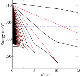
Figure 2: (Color online) Polariton branches at fixed in-plane vector $k_{\parallel}$ versus the magnetic field $B$ for a InAs/AlSb MQW structure embedded in a microcavity (black solid lines). Blue dotted–dashed line: bare cavity mode energy $E_{cav}$. Red dashed lines: ISB transition energies $\Delta E_{j}(B)$, plotted only in the $B$ range in which the corresponding LLs in the ground subband are not empty. For the parameters, see text.

In the non-parabolic case we have instead an ensemble of transitions at different $B$-dependent energies. In particular, since $m_{2}^{*}>m_{1}^{*}$, $\Delta E_{j}(B)$ decreases with $B$ for all $j$ values, as shown by red dashed lines in Fig. 2. The number of active ISB transitions is given by the number of filled LLs in the ground subband $n=1$, and thus also depends on $B$. In Fig. 2, each $\Delta E_{j}$ transition energy is in fact plotted versus $B$ only in the $B$ range for which the $E_{n=1,j}$ level is not empty, i.e. for $B<B_{j}=\frac{\pi\hbar n_{2D}}{e}\cdot\frac{1}{j}$ for $j\geq 1$ (while the $j=0$ LL is always filled).

In order to have a significant coupling with more than one ISB level, we choose a cavity geometry with a cavity mode energy $E_{\text{cav}}<E_{21}^{0}$ (blue dotted–dashed line of Fig. 2), so that in absence of coupling the photon energy crosses the bare ISB transition energies. In particular, in Fig. 2 we choose an effective cavity thickness $L_{z}=1.5$ $\mu$m and we set $\varepsilon_{\infty}=12.32$ for the dielectric constant of the InAs cavity. The in-plane wavevector is fixed to $k_{\parallel}=4.99$ $\mu$m^-1, corresponding to an angle of propagation inside the cavity of $\theta=67.2^{\circ}$ with respect to the $\hat{z}$ axis.

For the calculation of the polaritons, we note that each allowed transition channel $j$ is independent of the others and occurs at a different energy $\Delta E_{j}$ (for $B\neq 0$). We thus describe the polariton eigenstates (for a given in-plane $k_{\parallel}$ vector) as a linear combination of the state $|a\rangle$ with one photon in the cavity mode and no ISB excitations, and the set of states $|b_{j}\rangle$ with one ISB excitation associated to a given LL $j$ and no photons in the cavity. The coupling between the $|a\rangle$ and $|b_{j}\rangle$ states is then given by

$$\Omega_{j}=\tilde{\Omega}\sqrt{\frac{n_{j}}{n_{2D}}},$$ (3)

where $n_{j}$ is the population of the $j-$th LL in the ground subband (so that $\sum_{j}n_{j}=n_{2D}$). The frequency $\tilde{\Omega}$ is calculated in a way similar to the $B=0$ case:Ciuti et al. (2005)

$$\hbar\tilde{\Omega}=\sqrt{\frac{e^{2}\hbar^{2}n_{2D}n_{QW}E_{21}^{0}f_{21}\sin^{2}\theta}{2m_{0}\varepsilon_{0}\varepsilon_{\infty}E_{cav}L_{z}}}$$

where $f_{21}$ is the oscillator strength, which has been defined and calculated taking into account the non-parabolicity as described in Ref. Sirtori et al., 1994: $f_{12}=0.79\,m_{0}/m_{\Gamma_{6}}$ for our parameters. The calculated polariton branches are represented by black solid lines in Fig. 2. Note that, for a given value of $B$, we have included in the calculation only the $|b_{j}\rangle$ states originating from non-empty LLs.

The system parameters have been chosen in order to achieve a significant coupling between the cavity mode $|a\rangle$ and more than one ISB transition level $|b_{j}\rangle$. This can be achieved only if the coupling energy $\hbar\tilde{\Omega}$ is of the order of the typical deviation of the ISB transition energies with respect to $E_{21}^{0}$. In fact, if the coupling is much larger than the energy separation between the different ISB transitions, the latter ones behave essentially as a single degenerate level for what concerns the coupling with the cavity photons, and we then recover the ordinary two-level regime (not shown). In InAs/AlSb heterostructures, the ISB transition energy deviation is typically of the order of 10–15 meV at $B\approx 10$ T (see Fig. 2). For the parameters used in Fig. 2, the coupling $\hbar\tilde{\Omega}$ is about 5 meV. We notice moreover that the effects of the squared vector potential can be safely neglected in our structure, since the $A^{2}$ correction is of the orderCiuti et al. (2005) of $\hbar^{2}\tilde{\Omega}^{2}/E^{0}_{21}$, which is much smaller than cavity energy $E_{cav}$ (in our case $\hbar\tilde{\Omega}\ll E_{cav}\approx E^{0}_{21}$).

From Fig. 2 it is apparent that the polariton levels display a complex evolution as a function of the magnetic field. We distinguish three field regions. For large $B$ fields, where only the $j=0$ LL is filled, we recover the two-level correspondence, valid also for parabolic materials. As $B$ decreases, however, more LLs start to be filled and as a consequence, more ISB transitions couple to the light. At $B=B_{j}$ ($j\geq 1,2,\ldots$) a new state appears, which however has a zero coupling at this precise value of the magnetic field, since the corresponding LL is empty. Decreasing $B$, its population increases (while the populations of lower LLs decrease), so that the coupling is spread between the levels. Finally, in the $B\to 0$ limit, we end up with a bare cavity mode coupled to (and placed inside) a finite-width continuum of ISB transitions. As it is well known,Cohen-Tannoudji et al. (1998) the resulting eigenstates depend on the ratio between the continuum width and the coupling strength. Since in our case $\Delta E_{c}\approx 2\hbar\tilde{\Omega}$, two polariton states appear near each side of the bare ISB continuum limits (see Fig. 2 and discussion below).

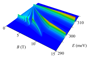
Figure 3: (Color online) Squared modulus of the “light” part of the polariton eigenvectors. Same parameters as in Fig. 2.

From the above discussion, we see that the magnetic field assumes the role of a real external control parameter, which can be used to tune the regime of light–matter interactions. To illustrate more clearly this point, we study also the eigenvector components of the polariton eigenstates. In Fig. 3 we show the squared modulus of the “light” part of the polariton eigenvectors, i.e. the component of the eigenvectors associated to the state $|a\rangle$. The magnitude of this component displays the three different regimes mentioned above. At large $B$ fields, we clearly identify the two polaritons resulting from the strong coupling between light and the $j=0$ ISB transitions. In the opposite $B$ regime, i.e. for small $B$ values, we see that the light component is mainly concentrated on the two extremal polariton branches. All other polaritons have a significantly smaller light component, and thus this regime resembles a two-level regime. Note however that all states have an influence on the overall coupling also in the $B\to 0$ limit, and therefore they cannot be disregarded in the calculation of the polariton coupling. Finally, there is a third regime for intermediate values of the magnetic field: in this case, the light is coupled with a discrete set of ISB states, and the resulting polariton branches have a similar magnitude of the light component.

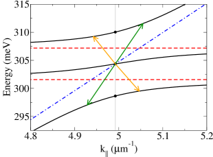
Figure 4: (Color online) Polariton branches as a function of the in-plane wavevector (black solid lines) for $B=B_{2}=5.17$ T. The blue dotted–dashed line (red dashed lines) represent the cavity mode ($j=0$ and $j=1$ ISB transitions) in absence of coupling. The vertical line indicates the $k_{\parallel}=k_{\parallel R}$ value (see text) at which Fig. 2 is calculated. Orange and green arrows: sets of entangled states in an optical parametric oscillator phenomenon (see text). Same parameters of Fig. 2.

To discuss more in detail the intermediate regime, we focus on a magnetic field $B=B_{2}=5.17$ T, which corresponds to a complete filling of the $j=0$ and $j=1$ LLs. Since the two LLs have the same population, Eq. (3) implies that the respective states $|b_{0}\rangle$ and $|b_{1}\rangle$ couple to the light with the same strength $\hbar\tilde{\Omega}/\sqrt{2}$. As a consequence of this and of the relative energy position of the uncoupled levels, the three resulting polaritons states have a similar magnitude of the light component, as it can also be deduced from Fig. 3. The dispersion of these three polaritons (at $B=B_{2}$) as a function of the in-plane wavevector $k_{\parallel}$ is shown in Fig. 4; the uncoupled cavity mode frequency and intersubband transitions are also shown with blue dotted–dashed and red dashed lines, respectively. The vertical line indicates the value of $k_{\parallel}$ used in Fig. 2.

The magnetic field control of the ISB polaritons might be observable in an optical experiment. For very strong $B$ fields (not discussed here) the cavity mode is energetically isolated, well above all the ISB levels, so that any spectrum probing the light component of the system eigenstates should reveal a single intense peak at the bare cavity energy. Decreasing to the high fields of Figs. 2 and 3 ($B\approx 15$ T), the optical spectrum is expected to display instead two peaks, characteristic of the strong ISB ($j=0$)–cavity coupling. The spectrum evolves then into three peaks of comparable intensities when decreasing the field to $B\approx B_{2}$. More peaks are expected to emerge when we further decrease $B$, if the broadening is small enough to allow to resolve them; the central peaks should decrease in amplitude as $B$ is further decreased, to the benefit of the two main lines at $B=0$.

Let us finally discuss an interesting aspect of the intermediate field region, resulting from the existence of multiple polariton lines. In Fig. 4, for $k_{\parallel}=k_{\parallel R}$ (vertical gray line) the cavity mode lays exactly at mid-distance from the two $j=0$ and $j=1$ ISB transitions. Moreover, since the bare cavity dispersion is to a good approximation a linear function of $k_{\parallel}$ around $k_{\parallel R}$, it can be easily shown that the resulting polariton dispersions $E_{m}(k_{\parallel})$ (with $m=1,2,3$ for the three branches) have the following interesting “mirror” property: they fulfill $E_{3}(k_{\parallel R}+k)+E_{1}(k_{\parallel R}-k)=2E_{2}(k_{\parallel R})$, with $k$ a small deviation from the resonance wavevector. Two of such sets of three-polariton states are pictured by green and orange arrows in Fig. 4. The three polaritons of each set are thus exactly phase-matched in both energy and wavevector spaces. Additionally, the upper and lower states have always identical group velocities, while all three waves velocities coincide for a particular value of detuning $k=k_{V}$ (orange arrows in Fig. 4). This might lead to improved non-linear optical response, like in the optical parametric oscillation phenomenon,Shen (2003) which has been studied in the literature in monolithic semiconductor microcavities exploiting exciton polaritonsSavvidis et al. (2000); Ciuti et al. (2001); Saba et al. (2001); Ciuti et al. (2003) and coupled microcavities.Diederichs et al. (2006) After pumping on the central state, entangled photon pairs (idler and signal) would be expected from the upper and lower branches. These latter would propagate along well-defined directions with respect to the pump beam, allowing an angular discrimination of the beams at the sample outcome (see below). Moreover, the generation would be polychromatic (even if possibly enhanced for $k=k_{V}$) above the frequency of separation between the two ISB bare transitions, with angular separation of colors in free space.

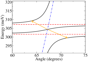
Figure 5: (Color online) Polariton branches for $B=B_{2}=5.17$ T as a function of the angle of the coupled light in the substrate. The blue dotted–dashed line (red dashed lines) represent the cavity mode ($j=0$ and $j=1$ ISB transitions) in absence of coupling. The orange arrows connect the same states as in Fig. 4. Same parameters of Fig. 2.

Of course, the present model is valid when the typical lifetimes of the cavity mode and of the electronic excitations are large enough to treat the different transitions independently. For what concerns the latter one, calculations performed in a similar systemFaugeras et al. (2006) show that the shortest lifetime (due to inelastic optical-phonon scattering) is larger than 1.5 ps, corresponding to a broadening of about 0.5 meV. The cavity mode lifetime can be tuned by tailoring the optical cavity; in typical experiments the cavity mode broadening is of the same order of the electronic excitations one.Dini et al. (2003) The different states in the intermediate and high-field regions are thus expected to be distinguishable in the experiments. Additionally, it is also worth recalling that in a typical reflectance spectroscopy measurement, photons with fixed $(E,k_{\parallel})$ propagate in the substrate (of index $n_{\text{sub}}$) with fixed angle $\theta$ (with respect to the layers normal) given by:

$$\sin\theta=\frac{\hbar c}{E\,n_{\text{sub}}}k_{\parallel}.$$

We show in Fig. 5 the energy versus $\theta$ plot for the polaritonic states around the resonance region of Fig. 4 ($n_{\text{sub}}=3.51$, as in the experiments of Ref. Anappara et al., 2007). The orange arrows connect the same states as in Fig. 4, i.e., those for which the central and generated polaritons have the same group velocities. As we can see, the angle difference is small (to ensure they all fall in the experimental light cone)Todorov et al. (2008) but sizeable (slightly less than 10 degrees), so that all three states, even though broadened, couple to an external mode and can thus be in principle revealed in an experiment.

The efficiency of the aforementioned non-linear process relies on inter-polariton interactions. In the context of exciton polaritons, polariton–polariton couplings have been previously studied.Combescot et al. (2007); Glazov et al. (2009); Vladimirova et al. (2010) The corresponding scattering matrix elements depend however on the peculiar properties of the exciton components of the polaritons. The study of the scattering processes for intersubband polaritons in the presence of non-parabolic dispersions is however beyond the scope of this work.

III Conclusion

In conclusion, we have shown that for intersubband polaritons in narrow-gap semiconductors, with a significant non-parabolicity, the magnetic field plays a true role of an external control parameter that allows to tune the regime of light–matter interactions. It becomes then possible to tune the strength of the coupling of the light with the different non-degenerate intersubband levels. We have reported numerical results for a InAs/AlSb system, and we have identified three different regimes for the polariton coupling as a function of the intensity of the magnetic field. Finally, we have presented a design for an optical parametric oscillator in the FIR spectral range. The structure is based on the existence of a mirror dispersion scheme for the magneto-polaritons, which ideally allows fulfilling phase-matching requirements for the pump and parametric waves.