Chemical evolution of protoplanetary disks – the effects of viscous accretion, turbulent mixing and disk winds

Abstract

We calculate the chemical evolution of protoplanetary disks considering radial viscous accretion, vertical turbulent mixing and vertical disk winds. We study the effects on the disk chemical structure when different models for the formation of molecular hydrogen on dust grains are adopted. Our gas-phase chemistry is extracted from the UMIST Database for Astrochemistry (Rate06) to which we have added detailed gas-grain interactions. We use our chemical model results to generate synthetic near- and mid-infrared LTE line emission spectra and compare these with recent Spitzer observations.

Our results show that if H₂ formation on warm grains is taken into consideration, the H₂O and OH abundances in the disk surface increase significantly. We find the radial accretion flow strongly influences the molecular abundances, with those in the cold midplane layers particularly affected. On the other hand, we show that diffusive turbulent mixing affects the disk chemistry in the warm molecular layers, influencing the line emission from the disk and subsequently improving agreement with observations. We find that NH₃, CH₃OH, C₂H₂ and sulphur-containing species are greatly enhanced by the inclusion of turbulent mixing. We demonstrate that disk winds potentially affect the disk chemistry and the resulting molecular line emission in a similar manner to that found when mixing is included.

1. Introduction

Protoplanetary disks are a natural and active environment for the creation of simple and complex molecules. Understanding their physical and chemical evolution is key to a deeper insight into the processes of star and planetary system formation and corresponding chemical evolution. Protoplanetary disks are found encompassing young stars in star-forming regions and typically disperse on timescales of less than a few million years (e. g., Haisch et al., 2001, 2006; Watson et al., 2007). Observations of thermal dust emission from these systems date back to the 1980s (see, e. g., Lada & Willking, 1984; Beckwith et al., 1990) and gave important insight into the structure and evolution of disks (see, e. g., Natta, 2007, for a review), however, inferring the properties of protoplanetary disks from dust continuum observations has several shortcomings: the dust component is only $\approx$ $1\%$ of the total mass contained in the disk and its properties are expected to change with dust growth and planet formation. Also, dust spectral features are too broad to study the disk kinematics (see, e. g., Carmona, 2010), and observations suggest that the gas and dust temperatures can differ considerably, particularly in the UV- and X-ray heated surface layers of the inner disk (e. g., Qi et al., 2006; Carmona et al., 2007).

The observation of molecular line emission from disks at (sub)mm wavelengths is limited by the low spatial resolution and sensitivity of existing facilities and target the rotational transitions of abundant molecules in the outer ($\geq 50\,\mathrm{AU}$) regions of the disk (see, e. g., Dutrey et al., 2007, for a review). Planet formation, however, most likely occurs at much smaller radii (Armitage, 2007). The superior sensitivity and spatial and spectral resolution of the Atacama Large Millimeter Array (ALMA), currently under construction, is required to observe the (sub)mm emission lines from the inner regions of protoplanetary disks in nearby star-forming regions to enable direct study of the physical and chemical structure of the inner disk.

Near- and mid-infrared observations, on the other hand, can probe the warm planet-forming regions (see, e. g., Najita et al., 2007, for a review). The $4.7\micron$ CO line emission has been detected at radii $<1\,\mathrm{AU}$, using, for example, Keck/NIRSPEC, Gemini/Phoenix and VLT/CRIRES (e. g., Carr, 2007; Pontoppidan et al., 2008; Brittain et al., 2009; van der Plas et al., 2009). The Spitzer Space Telescope has been used to spectroscopically study the inner disk at mid-infrared wavelengths. These observations show a rich spectrum of emission lines from simple organic molecules (e. g., Carr & Najita, 2008; Salyk et al., 2008; Pontoppidan et al., 2010) as well as from complex polycyclic aromatic hydrocarbons (PAHs) (e. g., Habert et al., 2006; Geers et al., 2006). They suggest high abundances of H₂O, HCN, C₂H₂ and provide evidence that the disk supports an active chemistry. C₂H₂ and HCN have also been detected in absorption towards IRS 46 and GV Tauri (Lahuis et al., 2006; Gibb et al., 2007). A particularly interesting case is CO₂, which has been reported to be abundant in the circumstellar disk of AA Tauri at $\sim 1.2\,\mathrm{AU}$ (Carr & Najita, 2008), in IRS 46 (Lahuis et al., 2006) and in several other sources (e. g., Pontoppidan et al., 2010), but which is not detected in the majority of sources observed by Spitzer. The recently launched Herschel Space Observatory and future space telescopes (e. g., the Space Infrared telescope for Cosmology and Astrophysics (SPICA) and the James Webb Space Telescope (JWST)) will enable the observation of molecular line emission in the mid- to far-infrared with unprecedented sensitivity and spectral resolution and will help address these controversial findings.

Due to increasing computational power, the theoretical study of the physical and chemical evolution of protoplanetary disks is entering its Golden Age. As a consequence of the observational limitations in the pre-Spitzer era, many numerical models focused only on the outer disk (e. g., Aikawa et al., 2002; Willacy, 2007). With the launch of Spitzer, however, the chemistry of the inner disk has increased in importance (e. g., Woods & Willacy, 2009). Unfortunately, complete models, including the physical and chemical evolution of the gas and the dust in the disk, coupled with a consistent treatment of the radiative transfer, is still beyond reach and several compromises have to be made.

One possibility is to ignore the chemical evolution and assume chemical equilibrium holds throughout the disk to investigate the physical structure in detail (e. g., Kamp & Dullemond, 2004; Jonkheid et al., 2004). Pioneering work by Gorti & Hollenbach (2004) and Nomura & Millar (2005) combined a basic disk chemistry with a self-consistent description of the density and temperature structure taking into account the gas thermal balance, the stellar irradiation and the dust grain properties. Recently, Woitke et al. (2009a) calculated radiation thermo-chemical models of protoplanetary disks, including frequency-dependent 2D dust continuum radiative transfer, kinetic gas-phase and photochemistry, ice formation and non-LTE heating and cooling. These studies show, in accordance with the observations, that the stellar UV and X-ray irradiation increases the gas temperature considerably in the surface layer of the disk, altering the disk chemistry drastically in this region.

Converse to that described above, several authors instead focused on combining the physical motion of material in the disk with time-dependent chemical network calculations (e. g., Aikawa et al., 1999; Markwick et al., 2002; Ilgner et al., 2004; Nomura et al., 2009). Radial inward motion due to the viscous accretion and vertical motion due to inherent turbulent mixing or disk winds have the potential to change the disk chemistry significantly, depending on the timescales of the transport processes. Molecules, initially frozen out on dust grains, can evaporate and increase the gas-phase abundances, provided that accretion and vertical mixing is comparable to, or faster than, the chemical reactions and the destruction by incident stellar irradiation. First steps towards including the accretion flow in the chemical network have been carried out by Aikawa et al. (1999), Markwick et al. (2002) and Ilgner et al. (2004). Nomura et al. (2009) calculated the effect of accretion along streamlines in steady $1$+$1$-dimensional $\alpha$-disk models for chemical networks containing more than 200 species. They found that the chemical evolution is influenced globally by the inward accretion process, resulting in, e. g., enhanced methanol abundances in the inner disk. Ilgner et al. (2004) also studied vertical mixing using the diffusion approximation and concluded that vertical mixing changes the abundances of the sulphur-bearing species. Their disk model, however, assumed the gas and dust temperatures were coupled everywhere in the disk and ignored stellar irradiation processes. Semenov et al. (2006) investigated gas-phase CO abundances in a 2D disk model, allowing for radial and vertical mixing using a reduced chemical network of 250 species and 1150 chemical reactions, and find the mixing processes strongly affect the CO abundances in the disk. Willacy et al. (2006) studied the effects of vertical diffusive mixing driven by turbulence and found that this can greatly affect the column density of various molecules and increase the size of the intermediate, warm molecular layer in the disk.

In this study, we consider the effects of inward accretion motion and vertical turbulent mixing to investigate to what extent the abundances of molecules such as H₂O, CO₂ and CH₃OH are affected in the inner disk. As an alternative driving force for vertical transport, we investigate the effect of upward disk winds on the disk chemistry. Several kinds of disk wind models, such as magnetocentrifugally driven winds (e. g., Blandford & Payne, 1982; Shu et al., 1994) and photoevaporation winds (e. g., Shu et al., 1993) have been suggested thus far. Recently, Suzuki & Inutsuka (2009) studied disk winds driven by MHD turbulence in the inner disk and found that large-scale channel flows develop most effectively at $1.5$–$2$ disk scale heights, i. e., approximately in those layers where molecular line emission is generated. The disk model in our study is from Nomura & Millar (2005) including X-ray heating as described in Nomura et al. (2007) and accounts for decoupling of the gas and dust temperatures in the disk surface due to stellar irradiation. We use a large chemical network and allow for adsorption and desorption onto and from dust grains. We also calculate mid-IR dust continuum and molecular line emission spectra assuming local thermodynamic equilibrium (LTE) and compare our results to recent observations. In Section 2 we describe our model in detail. In Section 3, we present and discuss our results, before drawing our final conclusions in Section 4.

2. Model

2.1. Disk structure

Our physical disk model is from Nomura & Millar (2005) with the addition of X-ray heating as described in Nomura et al. (2007). They compute the physical structure of a steady, axisymmetric protoplanetary disk surrounding a typical T Tauri star with mass $M=0.5M_{\odot}$, radius $R=2R_{\odot}$, effective temperature $T_{\mathrm{eff}}=4000\,\mathrm{K}$ and luminosity $L=0.87L_{\odot}$. We adopt the $\alpha$-disk model (Shakura & Sunyaev, 1973) to obtain the surface density profile from an equation for angular momentum conservation (e. g., Pringle, 1981, Eq. (3.9)). We assume an accretion rate of $\dot{M}=10^{-8}M_{\odot}\mathrm{yr}^{-1}$ and a viscosity parameter of $\alpha=0.01$.

We denote the radius in the cylindrical coordinate system with $s$ to distinguish it from the radial distance from the central star, i. e., $r=\sqrt{s^{2}+z^{2}}$, where $z$ represents the height from the disk midplane.

The disk is calculated between $s=0.01\,\mathrm{AU}$ and $300\,\mathrm{AU}$ in a $1+1$-dimensional model, which corresponds to a total disk mass of $2.4\cdot 10^{-2}M_{\odot}$ for the values of $\alpha$ and $\dot{M}$ given above. The steady gas temperature and density distributions of the disk are obtained self-consistently by iteratively solving the equations for hydrostatic equilibrium in the vertical direction and local thermal balance between heating and cooling of gas. To solve the equation for hydrostatic equilibrium (Nomura et al., 2007, Equation (11)), the condition

$$\int_{-z_{\infty}}^{+z_{\infty}}\rho_{\mathrm{gas}}(s,z)\,dz=\Sigma_{\mathrm{gas}}(s)$$ (1)

with $\rho_{\mathrm{gas}}(s,z_{\infty})=10^{-18}\mathrm{g}\,\mathrm{cm}^{-3}$ is imposed (Nomura & Millar, 2005). The heating sources of the gas are grain photoelectric heating by FUV photons and X-ray heating by hydrogen ionization, while cooling occurs through gas-grain collisions and by line transitions (for details, see Nomura & Millar 2005, Appendix A and Nomura et al. 2007).

The dust temperature is computed assuming radiative equilibrium between the absorption of stellar radiation and resulting thermal emission by the dust grains. Viscous heating is only taken into account in the disk midplane since its effects in the disk surface are comparably small for $\alpha=0.01$ (Glassgold et al., 2004). In the midplane, the density is high and the gas and dust temperature are tightly coupled. Note that it is often assumed that the gas temperature is coupled with the dust temperature everywhere in the disk. This is not true in the disk surface which is strongly irradiated by the parent star. The dust temperature is calculated using an iterative radiative transfer calculation by means of the short characteristic method in spherical coordinates, with initial dust temperature profiles obtained from the variable Eddington factor method (see Nomura, 2002; Dullemond & Turolla, 2000; Dullemond et al., 2002, for details).

The stellar X-ray and UV radiation fields are based on spectral observations of TW Hydrae, a classical T Tauri star. The X-ray spectrum is obtained by fitting a two-temperature thin thermal plasma model to archival XMM-Newton data (mekal model, $L_{\mathrm{X}}\sim 10^{30}\mathrm{erg}\,\mathrm{s}^{-1}$ for $0.1\,\mathrm{keV}\ldots 10\,\mathrm{keV}$) and is slightly softer than that of typical T Tauri stars with temperatures of about $2\,\mathrm{keV}$ in their quiescent phase (c. f., Wolk et al., 2005). The stellar UV radiation field has three components: photospheric blackbody radiation, hydrogenic thermal bremsstrahlung radiation and strong $\mathrm{Ly}\,\alpha$ emission ($L_{\mathrm{FUV}}\sim 10^{31}\mathrm{erg}\,\mathrm{s}^{-1}$ for $6\,\mathrm{eV}\ldots 13\,\mathrm{eV}$). The photochemistry used in this paper is described in detail in Walsh et al. (2010). Note that the scattering of $\mathrm{Ly}\,\alpha$ emission by atomic hydrogen is not taken into account. On the other hand, the $\mathrm{Ly}\,\alpha$ emission does not affect the molecular abundances significantly when the dust grains are well mixed with the gas (Fogel et al., 2011). We include the interstellar UV radiation field (Draine (1978) and van Dishoeck & Black (1982)), however, the interstellar UV and X-ray radiation fields are negligible compared to the central star (for details, see Nomura et al., 2007).

The mass density, gas temperature and dust temperature for our disk model are displayed in Figure 1, top, middle and bottom, respectively. A logarithmic spacing of the grid cells is adopted in radial direction, while the vertical structure is calculated on a linear grid. The number of grid cells used in this work is $35\times 30$ for $0.5\,\mathrm{AU}\leq s\leq 300\,\mathrm{AU}$ and $0\leq z/s\leq 0.8$. While this resolution is relatively coarse, its consequences for the line emission are limited due to the interpolation method during the line of sight integration (c. f., Section 2.7).

A more detailed description of the background theory and calculation of the disk physical model, along with further references, is given in Nomura & Millar (2005), Nomura et al. (2007) and Walsh et al. (2010).

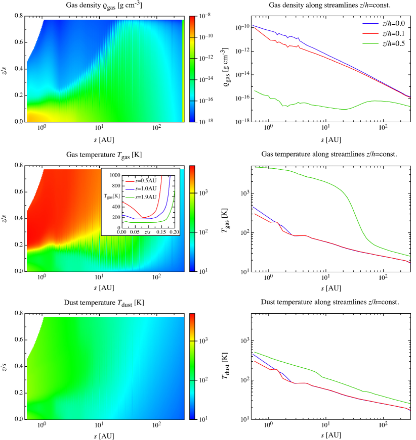
Figure 1.— From top to bottom: Gas density, gas temperature and dust temperature for the full disk model (left) and for constant streamlines $z/h$ of the viscous accretion (right), where $h$ denotes the scale height of the disk at radius $s$. For the gas temperature, inlaid are the vertical profiles as function of $z/s$ in the inner disk region.

2.2. Dust properties

The dust properties are important as they influence the physical and chemical structure of the disk in several ways. As the dominant source of opacity, they determine the dust temperature and the UV radiation field in the disk. They also affect the gas temperature, because photoelectric heating by UV photons is the dominant heating mechanism towards the disk surface. Further, the total surface area of the dust grains influences the molecular hydrogen abundance through the H₂ formation rates on grains and determines the freeze-out rate of chemical species onto the grain mantle throughout the disk (see Section 2.4). Finally, due to their dominant contribution to the opacity, the dust grain model also determines the emerging continuum spectrum.

For consistency, we adopt the same dust grain model for the spectral calculations as for the underlying protoplanetary disk (Nomura & Millar, 2005). We assume the dust grains to be compact and spherical, and to consist of silicate grains, carbonaceous grains and water ice. We further assume that the dust and the gas are well mixed and that the gas-to-dust mass ratio is uniform ($\rho_{\mathrm{dust}}/\rho_{\mathrm{gas}}=0.01$) in the disk. The size distribution is taken from Weingartner & Draine (2001a) to reproduce the observed extinction in dense clouds, with minimum and maximum sizes for the grains of $3.5$ Å and $\sim$$10\,\micron$, respectively. The heating of PAHs is included in the model for photoelectric heating (Weingartner & Draine, 2001b). For further details, see also Appendix D in Nomura & Millar (2005).

2.3. Gas-phase reaction network

For the calculation of the chemical evolution in the disk, we use a subset of the UMIST Database for Astrochemistry, or Rate06 (Woodall et al., 2007), neglecting only those species, and thus reactions, containing fluorine and phosphorus (Walsh et al., 2010). Since we are primarily interested in those regions where molecular line emission originates and where most molecules are in the gas phase, we neglect grain-surface reactions excepting H₂ grain formation (see Section 2.4). In summary, our gas-phase reaction network contains $375$ atomic, molecular and ionic species, ranging from atomic hydrogen H to relatively complex molecules such as H₃C₉N⁺ with mass $m=125\,\mathrm{u}$ (see Table 2.4 for a list of species of particular interest in this study and their binding energies on dust grains). The reaction network consists of $4346$ reactions including $3957$ two-body reactions, $214$ photochemical reactions, $164$ X-ray/cosmic-ray induced photoreactions and $11$ reactions for direct cosmic-ray ionization.

2.4. Gas-grain interactions

The formation of molecular hydrogen on the surface of dust grains is thought to be the most efficient means of forming H₂ directly from atomic hydrogen. Except for this process, we neglect grain-surface reactions of icy mantle species, but allow for adsorption onto and desorption from dust grains. Hence, except for atomic hydrogen, a particle that hits a dust grain can either detach without change or freeze out and remain in the icy grain mantle from where it may eventually evaporate. Atomic hydrogen forms H₂, freezes out onto the grain mantle or evaporates without reaction.

For the H₂ grain formation rates, we consider two different models. In model A, we refer to early work by Gould & Salpeter (1963) and Hollenbach & Salpeter (1971), who derive a grain formation rate for imperfectly shaped grain surfaces of

$$\dot{n}(\mathrm{H}_{2})^{\mathrm{gr}}_{\mathrm{A}} = \frac{1}{2}n_{\mathrm{H}}\cdot v_{\mathrm{H}}^{\mathrm{th}}(T_{\mathrm{gas}})n_{\mathrm{dust}}\pi\langle a^{2}\rangle\alpha_{\mathrm{H}}$$ (2)

$$= n_{\mathrm{H}}\cdot 2\cdot 10^{-18}\mathrm{s}^{-1}\ n_{\mathrm{tot}}\left(\frac{T_{\mathrm{gas}}}{300\,\mathrm{K}}\right)^{1/2}\!\!\!.$$

In Equation (2), $v_{\mathrm{H}}^{\mathrm{th}}(T_{\mathrm{gas}})$ is the thermal relative velocity of hydrogen atoms,

$$v_{\mathrm{H}}^{\mathrm{th}}(T_{\mathrm{gas}})=\left(\frac{8k_{\mathrm{B}}T_{\mathrm{gas}}}{\pi m_{\mathrm{H}}}\right)^{1/2}\!,$$ (3)

and $n_{\mathrm{dust}}\pi\langle a^{2}\rangle$ the cross section of the dust grains per unit volume, with $n_{\mathrm{dust}}\sim 6\cdot 10^{-10}n_{\mathrm{tot}}$ and $\langle a^{2}\rangle=4.84\cdot 10^{-12}\mathrm{cm}^{2}$ for the dust grain model adopted here. Further, $n_{\mathrm{tot}}$ and $n_{\mathrm{H}}$ denote the total number density of hydrogen nuclei and the number density of atomic hydrogen, respectively. The total number density of hydrogen nuclei is calculated from the mass density, $\rho_{\mathrm{gas}}$, using

$$n_{\mathrm{tot}}=\frac{\rho_{\mathrm{gas}}}{(1+4y_{\mathrm{He}})m_{\mathrm{H}}}=\frac{\rho_{\mathrm{gas}}}{1.4m_{\mathrm{H}}}\,,$$

where $y_{\mathrm{He}}=0.1$ is the fractional elemental abundance of helium. Here, we neglect the mass contained in other, less abundant elements.

Alternatively, in model B, the H₂ grain formation is calculated according to Cazaux & Tielens (2002),

$$\dot{n}(\mathrm{H}_{2})^{\mathrm{gr}}_{\mathrm{B}} = \dot{n}(\mathrm{H}_{2})^{\mathrm{gr}}_{\mathrm{A}}\cdot\varepsilon(T_{\mathrm{dust}})$$ (4)

$$= \frac{1}{2}n_{\mathrm{H}}\cdot v_{\mathrm{H}}^{\mathrm{th}}(T_{\mathrm{gas}})n_{\mathrm{dust}}\pi\langle a^{2}\rangle\alpha_{\mathrm{H}}\varepsilon(T_{\mathrm{dust}})\,,$$

with several updates for the efficiency $\varepsilon(T_{\mathrm{dust}})$ (Woitke 2009, private communication). The sticking coefficient, $\alpha_{\mathrm{H}}$, is taken from Hollenbach & McKee (1979), and approximated to first order, i. e.,

$$\alpha_{\mathrm{H}}\approx\frac{1}{1+0.4\sqrt{(T_{\mathrm{gas}}+T_{\mathrm{dust}})/100\,\mathrm{K})}}\,.$$ (5)

The model for adsorption of gaseous species onto dust grains and desorption of ice species from dust grains is taken from Woitke et al. (2009a), who consider collisional adsorption together with thermal desorption, cosmic-ray induced desorption and UV photodesorption.

We calculate the ice formation rates for all neutral and negatively charged species $k$ in our reaction network,

$$\dot{n}_{k\,\mathrm{ice}} = n_{k}R_{k}^{\mathrm{ads}}$$

$$-n_{k\,\mathrm{ice}}^{\mathrm{desorb}}\cdot\left(R_{k}^{\mathrm{des,\,th}}+R_{k}^{\mathrm{des,\,cr}}+R_{k}^{\mathrm{des,\,ph}}\right)\,,$$

where $n_{k\,\mathrm{ice}}$ denotes the number density of ice species $k$ and $n_{k\,\mathrm{ice}}^{\mathrm{desorb}}$ its fraction located in the uppermost surface layers of the ice mantle. This fraction $n_{k\,\mathrm{ice}}^{\mathrm{desorb}}$ is given by (Aikawa et al., 1996)

$$n_{k\,\mathrm{ice}}^{\mathrm{desorb}}=\left\{\begin{array}[]{ll}\displaystyle n_{k\,\mathrm{ice}}&\displaystyle n_{\mathrm{ice}}<n_{\mathrm{act}}\\[6.45831pt] \displaystyle n_{\mathrm{act}}\frac{n_{k\,\mathrm{ice}}}{n_{\mathrm{ice}}}&\displaystyle n_{\mathrm{ice}}\geq n_{\mathrm{act}}\,,\end{array}\right.$$ (7)

with $n_{\mathrm{act}}=3\cdot 10^{15}\cdot 4\pi\langle a^{2}\rangle n_{\mathrm{dust}}$ being the number density of active spots in the ice mantle, and $n_{\mathrm{ice}}$ being the number density of all ice species ($n_{\mathrm{tot}}=n_{\mathrm{gas}}+n_{\mathrm{ice}}$). In the following, we summarize the expressions for the rate coefficients and we refer readers to Woitke et al. (2009a) for a detailed discussion.

The adsorption rate for species $k$ with mass $m_{k}$ and thermal velocity $v_{k}^{\mathrm{th}}$ is

$$R_{k}^{\mathrm{ads}}=\pi\langle a^{2}\rangle n_{\mathrm{dust}}\alpha_{k}v_{k}^{\mathrm{th}}\,,$$ (8)

where we assume a sticking coefficient of unity for all species excepting hydrogen (c. f., $\alpha_{\mathrm{H}}$ in Equation (5)). The desorption rates are

$$R_{k}^{\mathrm{des,\,th}} = \nu_{k}^{\mathrm{osc}}\exp\left(-\frac{E_{k}^{\mathrm{bind}}}{T_{\mathrm{dust}}}\right)\,,\phantom{\int_{A}^{B}}$$ (9)

$$R_{k}^{\mathrm{des,\,cr}} = f_{70\,\mathrm{K}}R_{k,70\,\mathrm{K}}^{\mathrm{des,\,th}}\frac{\zeta_{\mathrm{CR}}}{5\cdot 10^{-17}\mathrm{s}^{-1}}\,,\phantom{\int_{A}^{B}}$$ (10)

$$R_{k}^{\mathrm{des,\,ph}} = \pi\langle a^{2}\rangle\frac{n_{\mathrm{dust}}}{n_{\mathrm{act}}}Y_{k}F_{\mathrm{FUV}}\,.\phantom{\int_{A}^{B}}$$ (11)

The binding energies $E_{k}^{\mathrm{bind}}\,[\mathrm{K}]$, for the most important species are listed in Table 2.4. The vibrational frequency of species $k$ in the surface potential well is

$$\nu_{k}^{\mathrm{osc}}=\left(\frac{3\cdot 10^{15}k_{\mathrm{B}}E_{k}^{\mathrm{bind}}}{\pi^{2}m_{k}}\right)^{1/2}\,.$$ (12)

The expression for cosmic-ray induced desorption is adopted from Hasegawa & Herbst (1993), who evaluate the rate coefficient at a temperature of $70\,\mathrm{K}$ with a duty cycle of the grains of $f_{70}=3.16\cdot 10^{-19}$. The photo-desorption yields $Y_{k}$ are simply set to $10^{-3}$ per UV photon (Westley et al., 1995). Finally, the cosmic ray ionization rate $\zeta_{\mathrm{CR}}$ and the FUV field $F_{\mathrm{FUV}}$ in units $[\mathrm{photons}/\mathrm{cm}^{2}/\mathrm{s}]$ are calculated from the density profile and the dust opacity adopted in the disk model (Nomura et al., 2007). The calculation of the FUV field is based on Nomura & Millar (2005, Equations (6) and (7)) and accounts for dust scattering.

Table 1Molecular binding energies $E^{\mathrm{bind}}[\mathrm{K}]$

species	$E^{\mathrm{bind}}[\mathrm{K}]$	reference
H	350	(5)
H2	450	(5)
CO2	2690	(3)
H2O	4820	(4)
CO	960	(1)
OH	1260	(5)
CH4	1080	(2)
NH3	3080	(4)
HCN	4170	(2)
CH3OH	2140	(5)
C2H2	2400	(2)
SO2	3070	(5)
H2S	1800	(5)

References. — (1) Sandford & Allamondola (1988), (2) Yamamoto et al. (1983), (3) Sandford & Allamondola (1990), (4) Sandford & Allamondola (1993), (5) Hasegawa & Herbst (1993)

2.5. Initial conditions

The initial abundances we use as input are listed in Table 2 and we calculate the chemical evolution over $10^{6}\,\mathrm{yr}$, the typical lifetime of protoplanetary disks. The initial abundances for each species $n_{k,k\,\mathrm{ice},0}$ include both the ice and the gas component.

We compare the freeze-out timescale $\tau_{k}^{\mathrm{ads}}$ and evaporation timescale $\tau_{k}^{\mathrm{des}}$ for each species in a simple model to determine whether it exists initially as gas or ice only:

$$\tau_{k}^{\mathrm{ads}}=\left(R_{k}^{\mathrm{ads}}\right)^{-1}\!\!,\qquad\tau_{k}^{\mathrm{des}}=\left(R_{k}^{\mathrm{des}}\right)^{-1}\!\!.$$ (13)

For $\tau_{k}^{\mathrm{ads}}<\tau_{k}^{\mathrm{des}}$, the species is initially frozen out, $n_{k\,\mathrm{ice}}=n_{k,0}$ and $n_{k}=0$. Otherwise, it exists in the gas phase only, $n_{k}=n_{k,0}$ and $n_{k\,\mathrm{ice}}=0$.

Table 2Initial fractional abundances in the chemical network, including the gas and ice component of each species.

species	$x_{k,0}$
H	2.00e-07
H+	1.00e-10
H${}_{3}^{+}$	1.00e-08
He+	2.50e-11
He	1.00e-01
CH4	2.00e-07
NH3	1.00e-05
H2O	1.00e-05
C2H2	5.00e-07
Si	3.60e-08
N2	2.00e-05
C2H4	1.00e-08
CO	5.00e-05
H2CO	4.00e-08
CH3OH	5.00e-07
O2	1.00e-06
H2S	1.00e-06
Fe+	2.40e-08

2.6. Physicochemical interactions: viscous accretion, turbulent mixing and disk winds

Modeling the physicochemical interaction is the key aspect of our study. Even with the steady increase in computational power, this is still a challenging problem which can only be overcome by massive parallel computing and by accepting several simplifications. In the context of a steady disk model, for example, it is a reasonable assumption to describe the interaction between the disk physics and chemistry as a one-way process. Hence, we consider the influence of physical processes on the disk chemistry, but neglect the feedback of the chemistry on the physical disk structure.

Despite this simplification, the calculation of the disk’s chemical evolution with interaction is still considerably more computationally expensive, the reason being that adjacent grid cells are chemically coupled through the radial and vertical exchange of material. Accordingly, their evolution must be calculated in parallel with integration time steps that can be shorter than the the time scale of the chemical reaction network, due to the Courant-Friedrichs-Lewy (CFL) condition (Courant et al., 1928) of the fluid (see Section 2.6.4). More precisely, to compute the models with interaction, we adopt the following procedure: all grid cells are initialized at the starting time with their initial conditions (Section 2.5) and the transfer coefficients between the grid cells are evaluated (see below for the calculation of these coefficients for the different transport processes). The chemical evolution of the entire disk is calculated in parallel for time steps that satisfy the CFL condition and the transport coefficients are updated each iteration. This step is repeated until a total age of the disk of $10^{6}\,\mathrm{yr}$ is reached.

In the following, we describe each process we consider in this study. A detailed discussion of the numerical methods used to compute the chemical evolution is given in Appendix A.

2.6.1 Radial transport by viscous accretion

Firstly, we allow for the radial inward transport of material through the disk via accretion. The main parameter describing this effect is the accretion rate $\dot{M}=10^{-8}M_{\odot}\mathrm{yr}^{-1}$, which relates the radial inflow velocity $v_{s}$ with the column density $\Sigma$ at radius $s$,

$$\dot{M}=2\pi sv_{s}\Sigma\quad(v_{s}>0\ \mathrm{for\ radial\ inflow})\,.$$ (14)

We assume that inward accretion occurs along streamlines $l=\sqrt{s^{2}+z^{2}}$, with $z/h=\mathrm{const}$. Here, $h$ is the scale height of the disk defined by $h=c_{\mathrm{s}}/\Omega_{\mathrm{K}}$, $c_{\mathrm{s}}$ is the sound speed at the disk midplane and $\Omega_{\mathrm{K}}$ is the Keplerian angular frequency.

We denote the net accretion rate of species $k$, i. e., the net change in its number density, with $\dot{n}_{k,\,\mathrm{acc}}$. In steady state, the net accretion rate of species $k$ can be written as (see Appendix A.1 for the numerical implementation)

$$\dot{n}_{k,\,\mathrm{acc}}=\frac{\partial(\tilde{A}n_{k}v_{l})}{\partial l}\,,$$ (15)

where $\tilde{A}$ is a geometrical factor and corresponds to $\rho_{i+1}/\rho_{i}$ in (A2). The boundary conditions for the accretion process at the inner and outer disk radii are set as follows: due to the purely inward motion, all material that flows inwards from the innermost grid cell is removed from the disk, whereas at the outer radius $s=300\,\mathrm{AU}$, the accretion timescales become sufficiently long that we can safely assume $\dot{n}_{k,\,\mathrm{acc}}=0$ for all species. In Section 2.6.4, we compare the timescales for viscous accretion with the chemical timescale and also with corresponding values for the other physical processes considered here.

2.6.2 Vertical transport by turbulent mixing

Although the mechanism is not yet fully clear, it is commonly understood that the source of viscosity in astrophysical disks is turbulence. Hence, a sufficiently large viscosity, as is the case in our model ($\alpha=0.01$) implies that the effect of turbulent mixing is strong, particularly in the inner disk region. While this turbulent mixing, in principle, occurs in the radial and vertical directions, we ignore the radial turbulent motion and focus on the vertical mass fluxes only. Furthermore, we assume that the turbulent velocity is independent of the distance $z$ from the midplane and thus only a function of radius.

We calculate the mixing in a diffusion-type approach. The diffusion coefficient is set as $K=v_{z}\,dz$, where

$$v_{z}=v_{z,\mathrm{mix}}=\alpha^{\prime}c_{\mathrm{s}}\,,$$ (16)

in analogy to the expression for the turbulent velocity in a Shakura-Sunyaev disk model, where the turbulent viscosity is

$$\nu_{\mathrm{turb}}=v_{\mathrm{turb}}l_{\mathrm{turb}}=\alpha c_{\mathrm{s}}h\,.$$ (17)

We assume $\alpha^{\prime}=10^{-3}$ to account for the turbulence in vertical direction only. For our numerical model, the length scale $dz$ corresponds to the vertical extent of the grid cells $\Delta z\approx h/30$. The mixing timescales are discussed in Section 2.6.4.

The usual diffusion equation for species k (c. f., Equation (3) in Willacy et al., 2006) reduces to

$$\dot{n}_{k,\,\mathrm{mix}}=\frac{\partial}{\partial z}\left(Kn_{\mathrm{tot}}\frac{\partial(n_{k}/n_{\mathrm{tot}})}{\partial z}\right)\,.$$ (18)

In Appendix A.2, we describe the numerical implementation of calculating the chemistry accounting for the mixing rates.

The boundary conditions are set at the disk midplane and surface. Due to the symmetry with respect to the midplane, the net exchange rate at $z=0$ is zero. Likewise, we assume that there is no exchange of material between the uppermost disk layer and any potential atmosphere on top of it.

2.6.3 Vertical transport by disk winds

We consider vertical disk winds as an alternative description of the vertical motion in the chemical model of the disk. Contrary to turbulent mixing, which implies upward and downward motion, the disk wind transports material upwards only (c. f. Figure 11(c) in Appendix A.2).

We refer to the wind solutions of Suzuki & Inutsuka (2009) to describe the vertical disk wind in our protoplanetary disk model. They investigated disk winds driven by MHD turbulence in local three-dimensional MHD simulations of stratified accretion disks and found that large-scale channel flows develop most effectively at $1.5$–$2$ disk scale heights, where the magnetic pressure is comparable to the gas pressure (here, we refer to their model with initial plasma $\beta=10^{6}$). The breakup of these channel flows drives structured disk winds, which might play an essential role in the dynamical dispersal of protoplanetary disks. While Suzuki & Inutsuka (2009) perform local three-dimensional simulations at radius $s=1\,\mathrm{AU}$ which lead to quasi-periodic cycles of $5$–$10$ rotations and strong mass outflows, our disk model is steady and does not allow for a dispersal of the disk.

We therefore adopt their solutions for the wind velocity $\hat{v}_{\mathrm{wind},0}$ at the midplane at $1\,\mathrm{AU}$ and calculate the radial and vertical profile according to Suzuki & Inutsuka (2009) and the vertical continuity equation in steady state, $\partial(\rho v_{z})/\partial z=0$,

$$v_{0} = v_{\mathrm{wind}}(s,z\!=\!0)=\varkappa\hat{v}_{\mathrm{wind},0}\cdot\frac{c_{\mathrm{s}}(s)}{c_{\mathrm{s}}(1\,\mathrm{AU})},$$

$$v_{z} = v_{\mathrm{wind}}(s,z)=v_{0}\cdot\frac{\rho(s,z=0)}{\rho(s,z)}\,,$$ (19)

where $\hat{v}_{\mathrm{wind},0}=8.5\cdot 10^{-5}c_{\mathrm{s}}(1\,\mathrm{AU})$ (Suzuki & Inutsuka, 2009). For large values of $\hat{v}_{\mathrm{wind},0}$, the midplane layers disperse over timescales shorter than the typical disk lifetime of $10^{6}\mathrm{yr}$, which contradicts the assumption of a steady disk model. We therefore introduce an ad-hoc factor $\varkappa=10^{-3}$ in Equation (19) to reduce the wind velocities such that the dispersal time scales, $\Sigma/(\rho_{\mathrm{gas}}v_{z})$ (where $\Sigma$ is the surface density of the disk), become $\sim 10^{6}\mathrm{yr}$. The resulting wind profiles reproduce the results of Suzuki & Inutsuka (2009) in the sense that the disk wind is most effective at $\sim 2$ disk scale heights, where the gas density and therefore the gas pressure decreases steeply and any potential magnetic pressure would become comparable with it.

The wind rates are calculated from the vertical continuity equation for species $k$, using the wind velocity profile (Equation (19)):

$$\dot{n}_{k,\,\mathrm{wind}}=-\frac{\partial(n_{k}v_{z})}{\partial z}\,.$$ (20)

The wind rates for the discrete grid of the disk are given in Appendix A.3.

The boundary conditions are set as follows: since we adopt small wind velocities so that the disk dispersal time becomes long enough, we can assume that the mass loss is negligible at the midplane and therefore $\dot{n}_{k,\,\mathrm{wind}}=0$, whereas at the upper boundary, we simply allow all material transported by the disk wind to be lost.

2.6.4 Timescales

The grid crossing times for the mass transport by viscous accretion, turbulent mixing and disk winds are displayed in Figure 2. These are set by the CFL-condition for the discrete grid of our disk model:

$$\tau_{\mathrm{acc}}=\frac{\Delta s}{v_{s}},\quad\tau_{\mathrm{mix}}=\frac{\Delta z}{v_{z,\,\mathrm{mix}}},\quad\tau_{\mathrm{wind}}=\frac{\Delta z}{v_{z,\,\mathrm{wind}}}.$$

The radial and vertical size of the grid cells are given by $\Delta s$ and $\Delta z$, respectively, and depend on distance $s$ from the star. For reference, we display the accretion, mixing and wind velocities in Figure 2 (left panel).

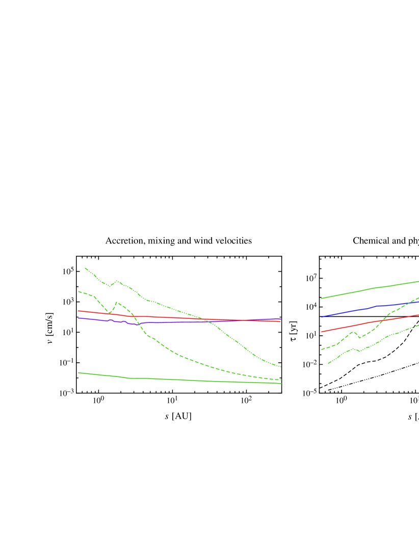
Figure 2.— Velocities (left) and timescales (right) for the transport processes of accretion (radial), mixing (vertical) and wind (vertical). Typical timescales of the photochemical reactions are also shown in the right panel (see text for details). Solid lines denote midplane values, i. e., $z/s=0$, (accretion, mixing, wind), or the timescale of the photochemistry for the interstellar radiation field (photochem.), respectively. Dashed lines correspond to $z/s=0.2$ and dotted-dashed lines to $z/s=0.5$.

In the right panel of Figure 2, we also plot the timescale of photochemistry given by (Duley & Williams, 1984):

$$\tau_{\mathrm{photochem}}=10^{3}\mathrm{yr}\cdot\frac{F_{\mathrm{FUV,ISRF}}}{F_{\mathrm{FUV}}(s,z)}\,,$$ (21)

where $F_{\mathrm{FUV,ISRF}}$ is the FUV photon flux of the interstellar radiation field. In the upper layers of the disk, the UV radiation field is strong and the timescale for the photochemistry is shorter than the dynamical timescales. Below the transition layer, $z/s\lessapprox 0.2$, the incident FUV radiation is highly attenuated and the chemical timescales are controlled by two-body reactions, which are sensitive to the temperature and density. The chemical timescale in this region is generally longer than the photochemical timescale for the interstellar radiation field, $10^{3}\mathrm{yr}$. The accretion and mixing timescales become comparable to this limit at $0.5$ and $10\,\mathrm{AU}$, respectively. The disk wind timescales are longer than the chemical timescales for all $z/s$ for the entire disk in this model.

2.7. Infrared molecular line spectra

Using the results of our chemical evolution calculations, we compute emergent mid-infrared spectra from the disk. We include the dust continuum, which is the dominant source of opacity in protoplanetary disks, along with molecular line emission and absorption, assuming local thermodynamic equilibrium (LTE).

The dust continuum opacities are taken from the Jena opacity tables, using routines contained within the RATRAN package (Ossenkopf & Henning, 1994; Hogerheijde & van der Tak, 2000). In accordance with the dust properties of the disk model, we use the tables for spherical dust grains (parameter “e5” in the RATRAN routines) with thin ice coating (parameter “thin”).

The HITRAN’2004 molecular spectroscopic database (Rothman et al., 2005) provides a large set of energy levels and line transitions in the infrared for 39 molecules, focussing on terrestrial atmospheric species. Nevertheless, the overlap of species of interest between the HITRAN and UMIST databases is sufficient for our purposes. Since isotopes are not currently included in our chemical reaction network, we neglect spectroscopic information for minor isotopes in the HITRAN database.

The major issue concerning the calculation of line intensities in the infrared is the limited availability of collisional coefficients, in particular, for the large set of levels and transitions contained in the HITRAN database (e. g., more than $180000$ transitions for the main isotope of CH₄ for wavelengths between $1$ and $40\,\micron$). Since the main purpose of this work is the calculation of the disk’s chemical evolution, a detailed non-LTE radiative transfer calculation of the emergent spectra is beyond the scope of this paper. We therefore assume local thermal equilibrium to model the line emission and absorption strengths for the species of interest. For a species k, the transition $j\to i$ ($E_{i}<E_{j}$) is calculated from the standard equations

$$Q_{k}(T_{\mathrm{gas}}) = \sum_{i}g_{k,i}\exp\left(-\frac{E_{k,i}}{T_{\mathrm{gas}}}\right)\,,$$ (22)

$$n_{k,i/j} = n_{k}\frac{g_{k,i/j}}{Q_{k}(T_{\mathrm{gas}})}\cdot\exp\left(-\frac{E_{k,i/j}}{T_{\mathrm{gas}}}\right)\,,$$ (23)

$$j_{k,ij} = h\nu A_{k,ji}n_{k,j}\mathcal{V}_{k}\,,\phantom{\int_{A}^{B}}$$ (24)

$$\kappa_{k,ij} = h\nu(B_{k,ij}n_{k,i}-B_{k,ji}n_{k,j})\mathcal{V}_{k}\phantom{\int_{A}^{B}}.$$ (25)

Here, $n$, $j$ and $\kappa$ denote the level populations, the line emissivity and the line opacity, respectively. The Einstein coefficients $A$ and $B$ are listed in the HITRAN database or determined using the principle of detailed balance. The database also provides statistical weights $g$ and partition functions $Q$ for a wide range of temperatures. We calculate Voigt profiles $\mathcal{V}$ including natural line broadening, pressure broadening and thermal broadening. A Doppler profile at a temperature, $T_{\mathrm{gas}}$, is assumed for the thermal broadening. Turbulent broadening is neglected, since it is negligible compared to thermal broadening for subsonic turbulent velocities. The half-widths for natural broadening $\gamma_{\mathrm{n}}$ and pressure broadening $\gamma_{\mathrm{p}}$ are provided by the HITRAN database at a temperature of $296\,\mathrm{K}$. The temperature dependence of pressure broadening is approximated by

$$\gamma_{\mathrm{p}}=\gamma_{\mathrm{p}}(296\,\mathrm{K})\cdot\left(\frac{296\,\mathrm{K}}{T_{\mathrm{gas}}}\right)^{n_{\mathrm{p}}}\!\!,$$ (26)

where $n_{\mathrm{p}}$ is the temperature-dependent exponent in the HITRAN database.

We adopt a simple, one-dimensional line-of-sight integration to calculate the emergent disk spectra for a disk viewed face-on, i. e., with an inclination $i=0$, relative to the observer. The radial resolution for the spectral calculation is identical to the chemical model. Along each ray, the intensity is integrated following the one-dimensional equation of radiative transfer, accounting for the thermal dust continuum emission and the molecular line emission,

$$\frac{dI_{\nu^{\prime}}}{dz}=(\nu^{\prime}/\nu)^{2}\Bigl{[}j_{\nu}-\kappa_{\nu}I_{\nu}\Bigr{]}\,.$$ (27)

Quantities on the right hand side of (27) are evaluated in the moving frame of a fluid element of the observed object, while those on the left hand side are given in the rest frame of the observer (denoted with ^′). The observed frequency is given by $\nu^{\prime}=\nu(1+(v/c)\cos\theta)$, where $v$ is the velocity of the fluid element and $\theta$ is the angle between the directions of the velocity and the observer. The emission and absorption coefficients are given by

$$j_{\nu} = \sum_{k}\sum_{E_{i}<E_{j}}j_{k,ij}+\kappa_{\nu,\mathrm{dust}}B_{\nu}(T_{\mathrm{dust}})\,,$$ (28)

$$\kappa_{\nu} = \sum_{k}\sum_{E_{i}<E_{j}}\kappa_{k,ij}+\kappa_{\nu,\mathrm{dust}}\,,$$ (29)

where $B_{\nu}$ is the Planck function and $\kappa_{\nu,\mathrm{dust}}$ is the specific dust absorption.

The total emission from the disk is calculated as

$$L_{\nu^{\prime},\,\mathrm{disk}}=8\pi^{2}\int s\,ds\,I_{\nu^{\prime}}(s)\,.$$ (30)

The full spectrum is obtained from

$$L_{\nu^{\prime}} = L_{\nu^{\prime},\,\mathrm{star}}+L_{\nu^{\prime},\,\mathrm{disk}}\phantom{\int}$$ (31)

$$= 4\pi^{2}R^{2}\cdot B_{\nu^{\prime}}(T_{\mathrm{eff}})+L_{\nu^{\prime},\,\mathrm{disk}}\,.$$

Here, the stellar emission is modeled as blackbody emission with temperature $T_{\mathrm{eff}}=4000\,\mathrm{K}$ and stellar radius $R=2R_{\odot}$ and is added to the dust continuum and molecular line emission from the disk.

For the line-of-sight integration, a volume-weighting method is adopted to interpolate the temperature and molecular densities before computing the emission and absorption coefficients. In doing so, potential effects of the relatively coarse grid on the emerging line emission are reduced.

3. Results and discussion

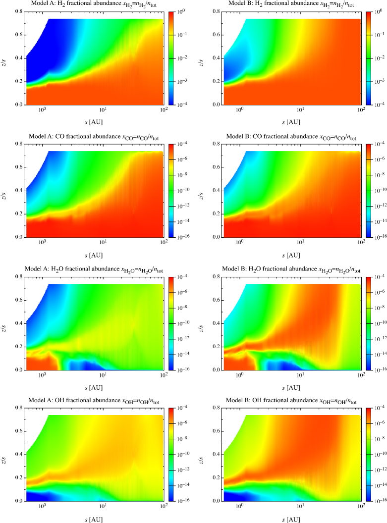
Figure 3.— Gas-phase fractional abundances of H₂, CO, H₂O and OH for models A and B.

In the following, we discuss the disk chemical evolution results and spectral calculations for the different models considered in this study. First, we investigate the influence of the H₂ formation rates on grains on the disk chemistry (Section 3.1). In Sections 3.2 and 3.3, we study the specific effects of viscous accretion, turbulent mixing and disk winds. Finally, in Section 3.4 we discuss how our results compare with observations of protoplanetary disks.

3.1. H₂ grain formation rates

Recently, Glassgold et al. (2009) studied the effect of the H₂ formation rates on dust grains on the water abundances at the disk surface of the inner disk. We revisit this effect and also study the influence on the infrared molecular line spectra.

In model A, we use the simple approximation from Gould & Salpeter (1963) and Hollenbach & Salpeter (1971). In model B, the adopted H₂ grain formation rate is that according to Cazaux & Tielens (2002) (see Section 2.4). In both models, the effects of accretion, turbulent mixing and disk winds are ignored. The chemical evolution of the disk is calculated over $10^{6}\mathrm{yr}$ for a radial range of $0.5$–$300\,\mathrm{AU}$. For both models, the chemical abundances everywhere in the disk have reached steady state by approximately $10^{5}\mathrm{yr}$.

In Figure 3, we show the resulting gas-phase abundances for molecular hydrogen, carbon monoxide, water and the hydroxyl radical for the inner $100\,\mathrm{AU}$ of the disk. In model B, the formation of molecular hydrogen is more efficient, particularly in the upper layers of the disk. In the warm molecular layer, i. e., the transition layer where the temperature rises and the density decreases steeply, H₂ is prone to continuous dissociation due to thermal reactions and incident radiation, and the enhanced grain formation rates in model B are able to maintain higher fractional abundances. Similarly, in the photodestruction region, i. e., the surface layers of the disk, H₂ is more abundant by a factor of $10$–$50$ between $5$ and $100\,\mathrm{AU}$. At even smaller radii the strong stellar UV radiation destroys H₂ on timescales shorter than it is formed even in model B. In the lower layers and outer regions of the disk, the differences between model A and B become negligible, since here, H₂ accounts for essentially all of the hydrogen nuclei.

The differences in the hydrogen chemistry also affect the resulting abundances of predominant molecules in the inner disk, particularly CO and H₂O. These molecules are commonly found in the planet-forming regions of protoplanetary disks (c. f., Salyk et al., 2008). Their modeled abundances depend strongly on the amount of molecular hydrogen at the disk surface and are therefore very different for model A and B. The increase of molecular hydrogen by a factor of $10$–$50$ between $5$ and $100\,\mathrm{AU}$ in the upper layers translates to an increase in CO and H₂O by a factor of $\approx 1000$. Such a strong correlation is expected theoretically (Glassgold et al., 2009): high fractional abundances of H₂ of $\sim 10^{-3}$ in the surface layers produce significant amounts of CO, H₂O and OH through a sequence of neutral radical reactions:

$$\mathrm{O}+\mathrm{H}_{2} \ \longrightarrow\ \mathrm{H}+\mathrm{OH}\,$$

$$\mathrm{OH}+\mathrm{H}_{2} \ \longrightarrow\ \mathrm{H}_{2}\mathrm{O}+\mathrm{H}\,$$

$$\mathrm{C}+\mathrm{OH} \ \longrightarrow\ \mathrm{CO}+\mathrm{H}\,.$$

Glassgold et al. (2009) show that the ratio $x(\mathrm{H}_{2}\mathrm{O})/x(\mathrm{O})$ depends quadratically on the ratio $x(\mathrm{H}_{2})/x(\mathrm{H}^{+})$. Our results confirm this correlation, since the $\mathrm{O}$ and $\mathrm{H}^{+}$ abundances are practically identical between model A and B.

The molecular column densities are only slightly changed compared with the fractional abundances, since the the latter are altered only at the disk surface where the density is low (Figure 4). Independent of the H₂ formation rate, gaseous CO traces the total disk mass, with a constant ratio $N_{\mathrm{CO}}/N_{\mathrm{H}_{2}}=10^{-4}$ at radii $<100\,\mathrm{AU}$ where the dust temperature is high enough so that CO does not freeze out. Gas-phase water is fairly abundant at radii $<3\,\mathrm{AU}$ (i. e., within the snow line of the disk) with $N_{\mathrm{H}_{2}\mathrm{O}}/N_{\mathrm{CO}}=0.25$. The column density of water is increased by about one order of magnitude between $5$ and $50\,\mathrm{AU}$, which is due to the large overabundance in the upper layers of model B.

The two H₂ formation rate models affect the abundances of the observable molecules in the warm molecular layer and the photodestruction layer, from where infrared molecular line emission originates. In Figure 5, we display the emergent spectra for a disk seen face on (inclination $i=0$). The spectral resolution is set to $600$ to match the Spitzer/IRS specifications. The molecular line emission is calculated for the following molecules between $1$ and $40\micron$: CO, H₂O, OH, CO₂, CH₄, NO, SO₂, NH₃, C₂H₂, N₂, H₂S, and NO⁺. The spectra differ substantially between the two models. Model A produces strong and narrow emission lines of OH between $10$ and $40\micron$, due to high abundances in the surface layers of the disk. On the contrary, H₂O shows broad emission bands between $5$ and $10\micron$, but only weak and narrow emission and absorption features at larger wavelengths, in contrast to the observations (c. f., Figure 1 in Carr & Najita, 2008). The CO emission band at $4$–$5\micron$ is present, as well as an absorption dip of CO₂ at $15\micron$. The absorption signatures are generated at radii $\lessapprox 2\,\mathrm{AU}$, where the temperature increases near the midplane due to viscous heating (c. f., the inlay in Figure 1). Since the abundances of CO₂ and H₂O in model A are high near the disk midplane, but low in the disk surface where the gas temperature increases towards an observer, absorption lines rather than emission lines are generated. Emission or absorption from other molecules included in the spectral calculation (e. g., NH₃, CH₄) is very weak in the spectrum.

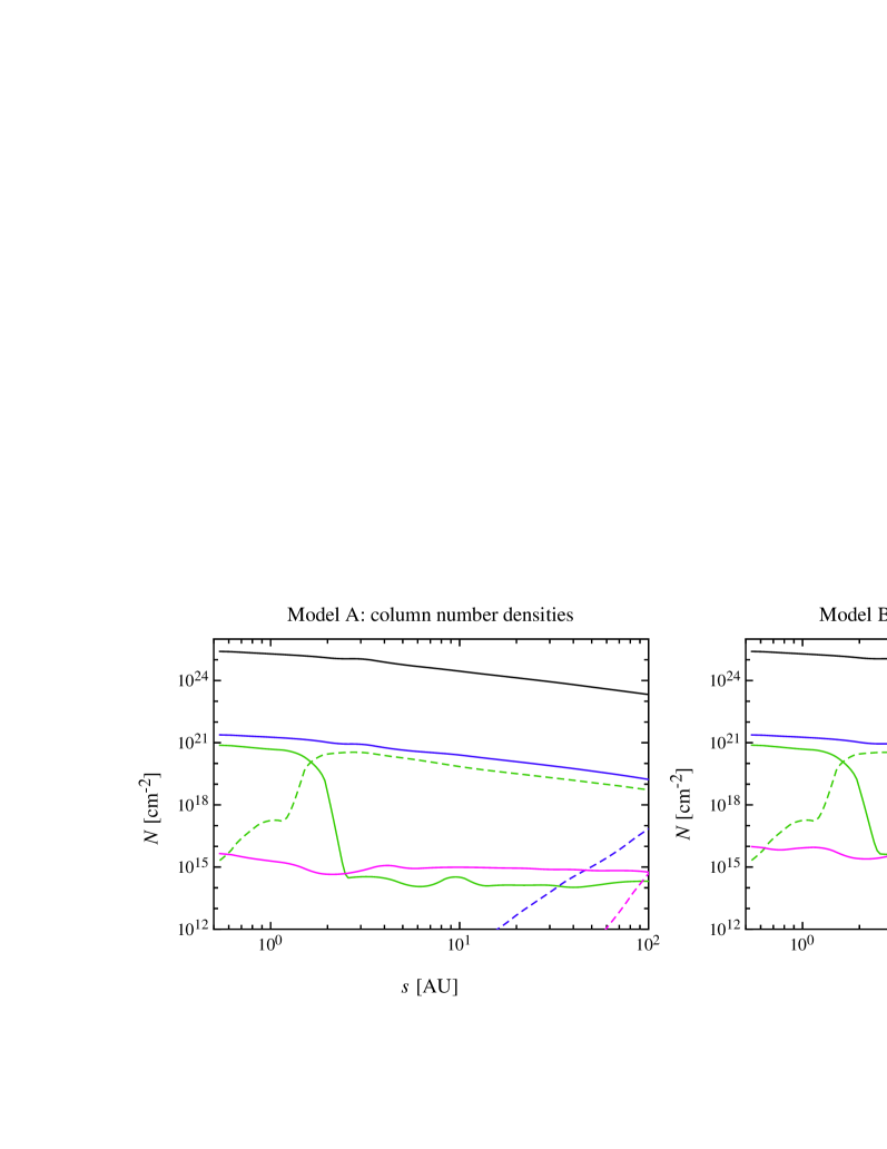
Figure 4.— Column densities for the species of interest in models A and B. Solid lines correspond to gas-phase species, dashed lines to ices.

Model B, on the other hand, produces a spectrum with enormous emission features from OH, H₂O and CO. The CO₂ absorption feature is not affected by the H₂ formation model, since it is destroyed very efficiently in the upper layers of the disk, where the main differences in the molecular abundances arise between model A and B. Comparing the two-dimensional abundances of OH, H₂O and CO in model A and B (Figure 3) allows us to constrain the origin of the emission lines to roughly $3$–$20\,\mathrm{AU}$, where the gas temperature is high enough to contribute to the total flux (c. f., Figure 1). Such strong emission features are certainly in disagreement with observations.

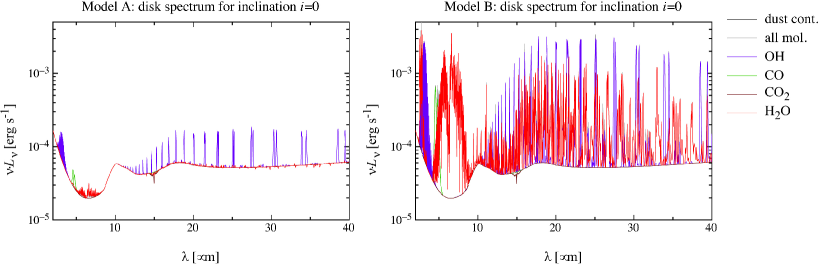
Figure 5.— Emergent LTE disk spectra for models A and B for dust continuum and molecular line emission.

The enhanced formation rate of H₂ on grains from Cazaux & Tielens (2002) might simply produce too much H₂ due to the choice of the variety of parameters used for this model, however, we should note here the limitations of our simple dust model. Firstly, we assume that gas and dust are well mixed in the disk, with a constant mass density ratio of $\rho_{gas}/\rho_{dust}\approx$ 100. Numerous studies show that dust grains will settle towards the midplane instead of residing in the upper disk layers (see, e. g., Dominik et al., 2007, for a review). Less dust grains in these layers lead to lower H₂ abundances and thus to lower abundances of water and OH. Aikawa & Nomura (2006) demonstrated that less dust grains will also lead to a lower gas temperature at the disk surface, which reduces the line intensities. Since the same line of argument applies to model A, it implies even lower abundances and thus weaker emission lines for H₂O in this model. Secondly, the spectral calculations in our study assume LTE level populations, which may overestimate the strength of the emission lines. Meijerink et al. (2009) studied the effects of non-LTE radiative transfer on the molecular emission lines of water: they assume fractional H₂O abundances between $10^{-10}$ and $10^{-4}$ throughout the disk. Interestingly, they conclude that a strong depletion at $s<1\,\mathrm{AU}$ is required to account for observed emission line spectra, and such a depletion is found in our model A. There, the H₂O abundance is low in the surface layer, because of the efficient destruction of water due to the stellar irradiation and the high temperature. Most important, however, is that Meijerink et al. (2009) find drastic differences between LTE and non-LTE spectral calculations: the LTE calculations overestimate the strength of the emission lines by a factor of $10$ for the strongest transitions (i. e., the largest Einstein coefficients). In model B, the line emission is generated in the upper layers of the disk, where the gas number density is of the order of $10^{8}\mathrm{cm}^{-3}$. The water line transitions between $10$ and $40\micron$ reported from Spitzer observations (e. g., Carr & Najita, 2008) are mainly rotational transitions in the ground vibrational state and in the first vibrational state with critical densities of $10^{12}\mathrm{cm}^{-3}$ or larger (Meijerink et al., 2009). Vibrational transitions between the two states that fall into this wavelength range have even higher critical densities. Hence, the conditions for LTE are partly violated and a proper non-LTE calculation of the disk spectra should be considered. In the following sections, we ignore the enhanced H₂ formation rates of model B and study the effects of accretion, turbulent mixing and wind on model A only.

3.2. Accretion, mixing, disk winds – single column solutions

To investigate the effects of including physicochemical interaction, we first focus on one vertical column of the disk at radius $s=1.3\,\mathrm{AU}$. Here, the temperatures of gas and dust are high enough, in particular in the upper layers of the disk, to allow for an active chemistry. Further, near- and mid-infrared observations derive characteristic radii for molecular line emission around $1\,\mathrm{AU}$ (c. f., Section 3.4).

In the following, we discuss in detail the modeled molecular abundances for a number of species of interest. For a better understanding, in particular for interpreting the resulting fractional abundances $x_{k}=n_{k}/n_{\mathrm{tot}}$, we display the physical properties of the disk column at this radius in Figure 6. The gas and dust temperatures are tightly coupled in the dense midplane with values around $200\,\mathrm{K}$. Hence, practically all species have desorbed from the dust grains and the ice abundances are negligible. In the warm molecular layer ($z\approx 0.2\,\mathrm{AU}$), the gas and dust temperatures begin to decouple due to the lower density. In the photodestruction layer, the gas is heated up to $4000\,\mathrm{K}$ because of the strong stellar irradiation, while the dust temperature is around a factor of $10$ lower.

In Figure 7, we plot the fractional abundances as a function of vertical distance from the midplane for the model without physicochemical interaction (model A) and for models with either accretion, turbulent mixing or disk winds (models ACR, MIX, WND). The gas-phase abundances are shown together with the – mostly negligible – ice abundances. All four models make use of the simple H₂ formation rates on grains (Eq. (2)), while model B (not displayed) includes the enhanced H₂ formation rates on grains (Eq. (4)) without physicochemical interaction. Table 3 at the end of this section compares the column densities of the most important species at radius $1.3\,\mathrm{AU}$ for all models A, B, ACR, MIX, WND. In the following, we discuss in detail the effects of turbulent mixing on the vertical chemical stratification at a radius $s=1.3\,\mathrm{AU}$, since this model has the largest effects on the chemical structure of the disk.

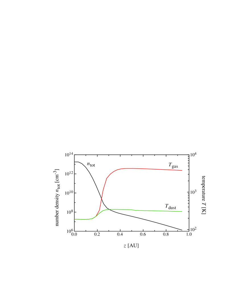
Figure 6.— Gas and dust temperature $T_{\mathrm{gas}}$ and $T_{\mathrm{dust}}$, and total number density $n_{\mathrm{tot}}$ as function of vertical distance from the disk midplane at a radius $s=1.3\,\mathrm{AU}$.

3.2.1 Turbulent mixing

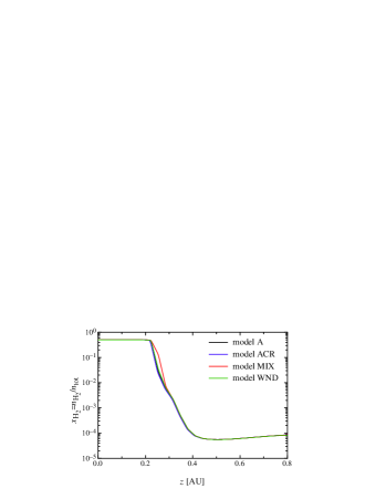
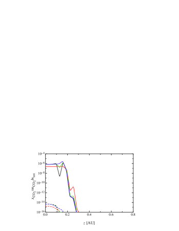
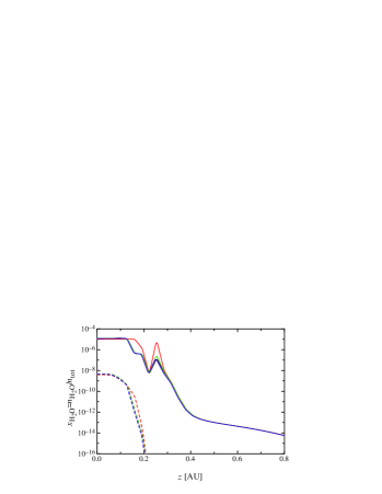
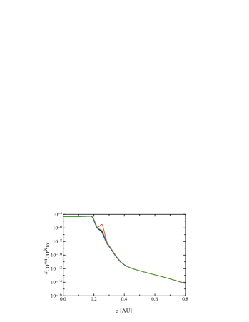
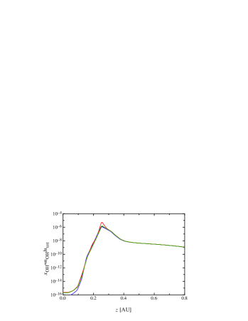
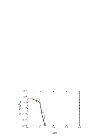
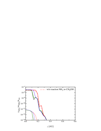
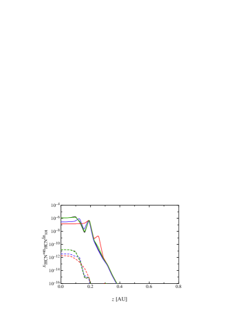
Figure 7.— Fractional abundance profiles of gas-phase species (solid) and ices (dashed) as a function of vertical distance from the midplane at $s=1.3\,\mathrm{AU}$ in model A (black), and in models with accretion (ACR, blue), mixing (MIX, red) or disk winds (WND, green).

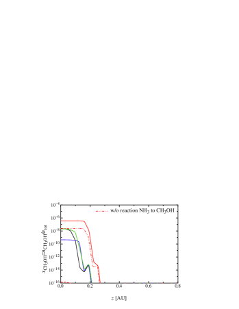
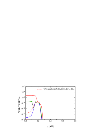
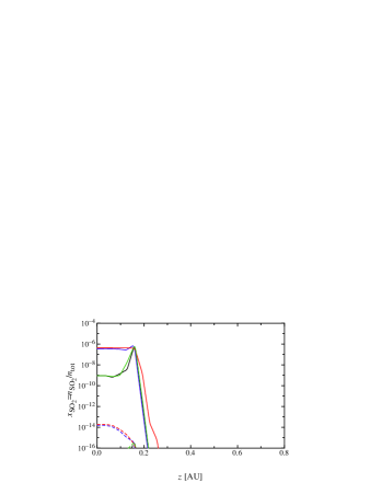
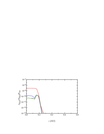
Figure 7.— (cont.) Gas and ice fract. abundances at $s=1.3\,\mathrm{AU}$.

Turbulent mixing has important effects on the disk’s chemical composition, in particular in the upper layers. Generally, diffusive mixing tries to homogenize the fractional abundances of molecules over the depth of the disk. Figure 7 illustrates this effect, for example in the case of H₂, the fractional abundances are slightly increased in the transition region, with only negligible changes in the column density (c. f., Table 3 at the end of this section).

This effect is more pronounced for CO₂: in model A, CO₂ is abundant close to the midplane only, since it is removed from the upper layers by reactions with H and H⁺ and by photo-dissociation due to the incident UV and X-ray radiation:

$$\mathrm{H}+\mathrm{CO}_{2} \ \longrightarrow\ \mathrm{CO}+\mathrm{OH}\,$$

$$\mathrm{H}^{+}+\mathrm{CO}_{2} \ \longrightarrow\ \mathrm{HCO}^{+}+\mathrm{O}\,$$

$$\mathrm{CO}_{2}+\gamma_{\mathrm{UV}} \ \longrightarrow\ \mathrm{CO}+\mathrm{O}\,$$

$$\mathrm{CO}_{2}+\gamma_{\mathrm{X-ray}} \ \longrightarrow\ \mathrm{CO}+\mathrm{O}\,.$$

At $z\approx 0.2\,\mathrm{AU}$, the reactions with H⁺ and the X-ray photochemistry are dominant, while in the upper layers, the UV photochemistry is most important. In model MIX, CO₂ diffuses upwards and its abundance is reduced near the midplane.

The H₂O, OH, and CO abundances are correlated with that of molecular hydrogen and are enhanced in model MIX in the region where H₂ is more abundant. The effect of diffusion of H₂O leads to reduced fractional abundances for $z<0.15\,\mathrm{AU}$ and increased abundances between $0.15\,\mathrm{AU}$ and $0.2\,\mathrm{AU}$. Water is destroyed easily at high temperatures and through photodissociation by UV and X-ray photons. The H₂O abundance has a dip at $z\approx 0.22\,\mathrm{AU}$, where both the gas temperature and density are relatively low (c. f., Woitke et al., 2009b, Figure 1). Here, UV and X-ray photodestruction become strong, while at the same time the temperature is still too low to activate the main formation reactions for H₂O,

$$\mathrm{H}_{2}+\mathrm{O} \ \longrightarrow\ \mathrm{OH}+\mathrm{H}\,$$

$$\mathrm{OH}+\mathrm{H}_{2} \ \longrightarrow\ \mathrm{H}_{2}\mathrm{O}+\mathrm{H}\,.$$

In the case of methane, diffusion also increases the fractional abundances in the surface layers. At the same time, the formation of CH₄ close to the midplane is efficient enough to maintain its initial fractional abundance, leading to an overall increase in the column density of methane. For $z\geq 0.3\,\mathrm{AU}$, methane is destroyed quickly by UV and X-ray photons.

A similar mechanism is responsible for the considerable increase in ammonia for $z\leq 0.3\,\mathrm{AU}$. The formation of ammonia near the disk midplane is driven by a change in the oxygen chemistry, with O₂ being overabundant in model MIX (see also Section 3.3). The differences in the oxygen abundance between model A and model MIX is caused by the continuous diffusion of O₂ from the warm molecular layer towards the midplane. This implies a decrease in the column density of HCN, whose formation is competing with NH₃ for the available nitrogen. Since the number of nitrogen atoms over the full column is conserved and since the formation of NH₃ is more efficient, HCN is depleted by one order of magnitude close to the midplane, compared with that in model A. Its column density decreases by approximately the amount required for the formation of the additional ammonia molecules.

The most pronounced effect arises in the case of methanol as a consequence of the increase in ammonia. Its fractional abundance increases for $z\leq 0.3\,\mathrm{AU}$ by one to six orders of magnitude, resulting in a column density of $1.2\cdot 10^{19}\mathrm{cm}^{-2}$ compared with $4.7\cdot 10^{17}\mathrm{cm}^{-2}$ in model A. This is due to an enhanced production of CH₃OH by the reaction (Rodgers & Charnley, 2001)

$$\mathrm{CH}_{3}\mathrm{OH}_{2}^{+}+\mathrm{NH}_{3} \ \longrightarrow\ \mathrm{NH}_{4}^{+}+\mathrm{CH}_{3}\mathrm{OH}\,.$$

In Figure 7, we display the ammonia and methanol abundances for an additional model calculation with diffusive mixing, but where this reaction is switched off. The ammonia abundances remain unchanged, but the methanol abundances drop by one order of magnitude, which is comparable to the midplane abundances in model A.

Significant changes are also found for acetylene, C₂H₂. At $z=0.2\,\mathrm{AU}$, it is mainly produced from NH₃ by the reactions

$$\mathrm{NH}_{3}+\mathrm{C}_{2}\mathrm{H}_{3}^{+} \ \longrightarrow\ \mathrm{C}_{2}\mathrm{H}_{2}+\mathrm{NH}_{4}^{+}$$

$$\mathrm{NH}_{3}+\mathrm{C}_{2}\mathrm{H}_{2}^{+} \ \longrightarrow\ \mathrm{C}_{2}\mathrm{H}_{2}+\mathrm{NH}_{3}^{+}\,,$$

as well as by a reaction of C and CH₃ at $z<0.2\,\mathrm{AU}$,

$$\mathrm{C}+\mathrm{C}\mathrm{H}_{3} \ \longrightarrow\ \mathrm{C}_{2}\mathrm{H}_{2}+\mathrm{H}\,.$$

Switching off these reactions leads to a significant decrease in C₂H₂ (c. f., Figure 7). Hence, acetylene profits from the increase in ammonia abundances and is overabundant by two orders of magnitude at $z\leq 0.2\,\mathrm{AU}$. Higher up in the disk, it is destroyed efficiently by photochemical reactions and reactions with atomic hydrogen.

Finally, we inspect the sulphur-bearing species SO₂ and H₂S. Initially, sulphur is locked in H₂S only, with a fractional abundance of $10^{-6}$ (c. f., Table 2). H₂S is easily destroyed by atomic hydrogen due to the small activation barrier of this reaction. Provided the O₂ and OH abundances are sufficiently high, this drives a chain of reactions (Charnley, 1997; Millar et al., 1997) which forces large amounts of H₂S into SO₂ in both models at $z\leq 0.25\,\mathrm{AU}$. The now highly abundant SO₂ near the midplane is destroyed on timescales longer than its formation timescales and therefore provides a steady reservoir to maintain the enhanced H₂S abundances in comparison to model A. At the midplane, the destruction of H₂S is less efficient, but still sufficient to produce OCS from CO and S (Hatchell et al., 1998). After $10^{6}\mathrm{yr}$, sulphur is locked in SO₂ and OCS in equal amounts.

Contrarily, in model A, the formation of SO₂ is inefficient in the lower layers due to the missing OH and the missing O₂ at $z\approx 0$. Thus, the slower reaction path of S with CO is preferred and OCS is built up over the lifetime of the disk, eventually locking all sulphur.

3.2.2 Disk winds

The resulting chemical abundances for model WND are displayed in Figure 7. For all species, the effects of the disk wind on the vertical stratification of the chemical species are much less pronounced than in the case of turbulent mixing. In the cases of CO₂, NH₃, CH₃OH and C₂H₂, slight increases in the fractional abundances are found around $z=0.2\,\mathrm{AU}$, in particular where narrow dips occur in the abundances from model A. Protected by the upper layers against the UV and X-ray irradiation, molecules transported upwards from the midplane fill these sinks on timescales comparable to their removal by chemical reactions.

The reason for the inefficiency of the disk wind lies in the steady disk model assumption considered here: to avoid disk dispersal over the lifetime of the disk, which would contradict the steady state assumption, we introduced a scaling factor $\varkappa=10^{-3}$ for the resulting wind speeds of Suzuki & Inutsuka (2009) at the midplane layer. Hence, the upward velocities near the midplane are low in model WND, compared to the turbulent velocities in model MIX (c. f., Figure 2). At radii $s\leq 10\,\mathrm{AU}$, the wind velocities become very large in the photodestruction region of the disk ($z/s>0.3$), due to the continuity equation in vertical direction in steady state. But there, the timescales of the photochemistry are extremely short so that the effect of the disk wind is small (c. f., Figure 2).

For a scaling factor $\varkappa=10^{-3}$, the midplane grid cell at radius $s=1.3\,\mathrm{AU}$ evaporates in about $2\cdot 10^{5}\mathrm{yr}$, corresponding to a mass loss of $20\%$ of the total mass contained in this disk ring. Hence, in a stationary model, $\varkappa$ should be lower than $10^{-3}$, which would lead to even less efficient disk winds.

We thus conclude that in a steady disk model, the disk winds have only negligible effects. Due to the necessary downscaling of the wind speeds by a factor of $1000$ ($\varkappa=10^{-3}$), the vertical mass transport becomes small and causes only small changes in the disk’s chemical composition. Nonetheless, it is worth noting that in a time-dependent physical disk model, where evaporation and dynamical refueling by the accretion flow are allowed, the disk wind may become significant. The simple model considered here suggests that it will affect molecules that also show an enhancement in the upper layers in the diffusive mixing model (e. g., NH₃, CH₃OH).

3.2.3 Viscous accretion

The chemical abundances from model ACR at a radius of $1.3\,\mathrm{AU}$ are displayed in Figure 7. As in the previous cases, at the disk surface photochemistry dominates and the accretion flow does not affect the chemical composition. Close to the disk midplane, the accretion time scale is comparable to the chemical timescale and the effects of the radial inflow of material become visible. Whether the accretion flow leads to an increase or a decrease in the abundance of a particular species depends on the formation and destruction timescales of that species. In the case of H₂O, for example, the chemical reactions are fast enough to compensate for the effects of the accretion flow and the abundances and column density are similar to those from model A.

On the contrary, NH₃ shows higher abundances at $z<0.15\,\mathrm{AU}$. As discussed for the case of diffusive mixing above, the total amount of nitrogen atoms is conserved and determined by the initial abundances of N₂ and NH₃ (c. f., Table 2). An increase in the column density of NH₃ from $2.5\cdot 10^{20}\mathrm{cm}^{-2}$ in model A to $3.4\cdot 10^{20}\mathrm{cm}^{-2}$ in model ACR leads to a decrease in HCN from $4.3\cdot 10^{19}\mathrm{cm}^{-2}$ to $1.1\cdot 10^{19}\mathrm{cm}^{-2}$ at this radius.

In contrast to the results from model MIX, methanol shows lower abundances close to the disk midplane, despite the increase in ammonia. Since its fractional abundance is even lower than those from model A, the reason, therefore, is not only the lack of vertical diffusion, but the fact that the formation and evaporation timescales (from dust grains) of methanol at around $10\,\mathrm{AU}$ are longer than its destruction timescale (c. f., Section 3.3). The accretion flow propagates this depletion inwards over time. Compared to model A, this reduces the CH₃OH column density from $4.7\cdot 10^{17}\mathrm{cm}^{-2}$ to $1.4\cdot 10^{16}\mathrm{cm}^{-2}$.

One should bear in mind that the location of the snow line for methanol and hence its gas-phase abundance is sensitive to its binding energy on dust grains, which varies across the literature. Here, we adopt the theoretical value from Hasegawa & Herbst (1993), $E_{\mathrm{bind}}=2140\,\mathrm{K}$. Sandford & Allamondola (1993) and more recently Brown & Bolina (2007) find much higher values between $4000$ and $5000\,\mathrm{K}$ based on the results of temperature-programmed desorption (TPD) experiments on pure methanol ice. Higher binding energies would imply lower gas-phase abundances and a shift of the snow line to smaller radii. Here, the NH₃ abundances are higher and the formation of methanol more efficient, which would imply higher gas-phase abundances within the snow line.

A similar decrease in the abundances in the innermost disk can be found particularly for C₂H₂, where the accretion flow removes a considerable fraction of acetylene close to the midplane (c. f., Table 3 for the resulting column densities of C₂H₂ and other species).

Table 3Calculated column densities $N[\mathrm{cm}^{-2}]$ at radius $s=1.3\,\mathrm{AU}$ of selected species for the disk models considered in this study.

species	A	B	ACR	MIX	WND
H2	1.7e+25	1.7e+25	1.7e+25	1.7e+25	1.7e+25
CO2	2.5e+19	2.6e+19	2.5e+19	8.3e+18	2.4e+19
H2O	4.2e+20	4.2e+20	4.0e+20	3.5e+20	4.2e+20
OH	1.5e+15	9.3e+15	1.5e+15	5.3e+15	1.8e+15
CO	1.6e+21	1.6e+21	1.6e+21	1.7e+21	1.6e+21
CH4	5.4e+18	5.4e+18	6.5e+17	7.1e+18	5.7e+18
NH3	2.5e+20	2.5e+20	3.4e+20	3.0e+20	2.6e+20
HCN	4.3e+19	3.8e+19	1.1e+19	4.7e+18	4.0e+19
CH3OH	4.7e+17	4.8e+17	1.4e+16	1.2e+19	5.6e+17
C2H2	1.6e+16	1.6e+16	1.3e+14	2.2e+18	1.6e+16
SO2	2.7e+17	2.6e+17	1.2e+19	1.4e+19	2.9e+17
H2S	9.6e+14	8.3e+17	6.2e+15	2.8e+18	9.4e+14
OCS	3.3e+19	3.2e+19	2.0e+19	1.6e+19	3.3e+19

3.3. Accretion, mixing – full disk solutions

In the previous section, we inspected in detail the chemical abundances for the different disk models as a function of height at a single radial position. The chemical composition varies between the individual models due to mass transport in the radial and vertical directions. The results thereby depend strongly on the species considered, in particular, on its formation and destruction timescales relative to the dynamical timescales. Since these timescales vary with radial distance from the star for accretion, turbulent mixing and disk winds, we expect significant changes in the effects of these mass transport phenomena at different radial positions in the disk.

Here, we focus on the radial accretion and vertical mixing and neglect the disk wind. At a radius, $s=1.3\,\mathrm{AU}$, the influence of the disk wind on the chemistry is small, compared with diffusive mixing, due to the low wind speed required to impede the evaporation of the disk in our model. At larger radii, the wind velocities are even smaller, leading to longer timescales of the upward wind motion. At the same time, however, the chemical timescales increase (c. f., Section 2.6.4), so that we do not find significant changes to the disk chemistry due to the inclusion of a disk wind.

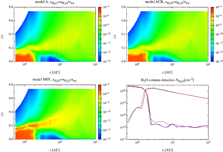
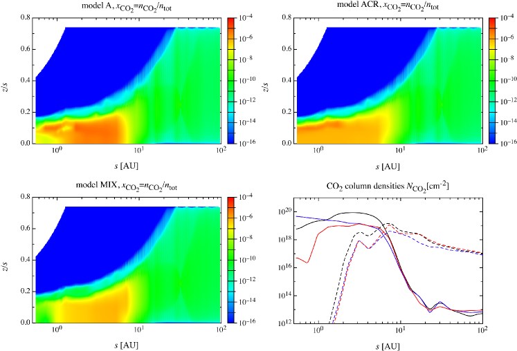
Figure 8.— Two-dimensional fractional gas-phase abundances and column densities (solid: gas; dashed: ice) of H₂O and CO₂ for model A (black), model ACR (blue) and model MIX (red).

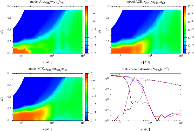
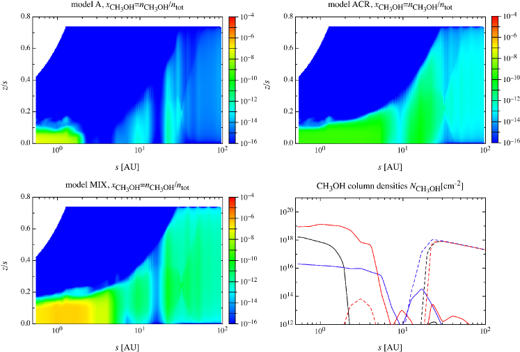
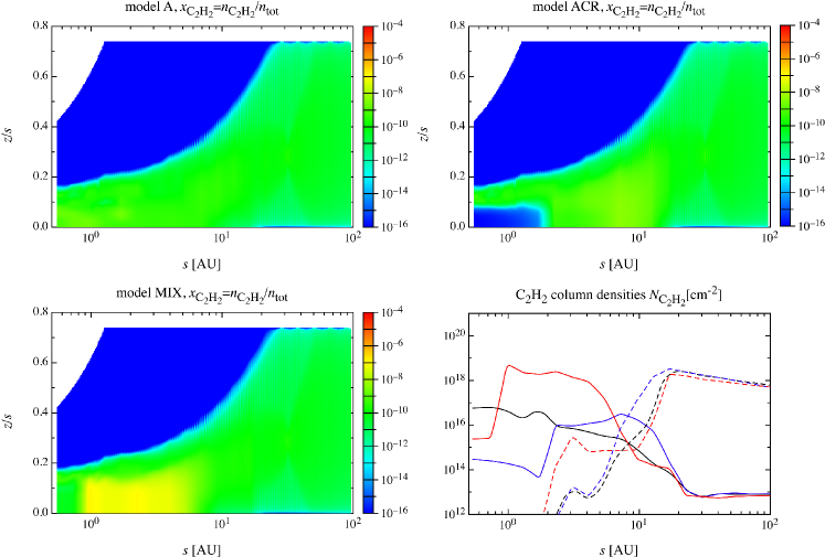
Figure 8.— (cont.) Two-dimensional fractional gas-phase abundances and column densities (solid: gas; dashed: ice) of NH₃ and CH₃OH for model A (black), model ACR (blue) and model MIX (red).

Figure 8.— (cont.) Two-dimensional fractional gas-phase abundances and column densities (solid: gas; dashed: ice) of C₂H₂ for model A (black), model ACR (blue) and model MIX (red).

We compare the resulting fractional gas-phase abundances and the gas and ice column densities for model ACR and model MIX with model A in Figure 8. The results for water differ only slightly between the models, and the only difference arises in a narrow stripe $z/s\approx 0.2$–$0.4$, where the gas-phase abundances of water are increased in model MIX due to the enhanced H₂ abundances (see also the discussion in Section 3.1). This leads to an increase in the gas-phase column density between $2$ and $10\,\mathrm{AU}$. Since the H₂O abundances are increased in the transition layer, turbulent mixing affects the strength of the H₂O line emission from the disk. This can be seen in Figure 9, where we compare the emerging disk spectra for model A, model ACR and model MIX. Apart from H₂O, the species dominating the molecular line emission are CO and OH. Both show slightly stronger emission lines in model MIX and in model ACR, although the effect is more pronounced in the case of diffusive mixing.

In the case of CO₂, turbulent mixing reduces the gas-phase column density inside $10\,\mathrm{AU}$: turbulent mixing leads to the diffusion of CO₂ from the lower, protected layers into the upper disk, where it is efficiently destroyed by incident radiation, compared with its production. For radii $\leq 1\,\mathrm{AU}$, CO₂ is strongly depleted. Viscous accretion, on the other hand, enhances the CO₂ gas-phase abundances at radii $\leq 1\,\mathrm{AU}$ due to a net inward transport from radii $\leq 10\,\mathrm{AU}$. This leads to changes in the disk spectra for both models ACR and MIX: inside $2\,\mathrm{AU}$, the gas and dust temperature first decrease with increasing distance from the midplane (see Figure 1). This is due to the viscous heating near the midplane. Since CO₂ is concentrated near the midplane and since it is abundant in model ACR (depleted in model MIX), the absorption feature at $15\micron$ is enhanced (reduced).

Ammonia shows the largest variations between the different models. Compared to model A, model ACR and model MIX lead to a similar increase in the gas and ice abundances between $1$ and $10\,\mathrm{AU}$. The increase in ammonia is a result of a fundamental change in the oxygen chemistry. In model ACR and model MIX, atomic oxygen is reduced by orders of magnitude between $2$ and $10\,\mathrm{AU}$, with an increase in O₂ and a decrease in OH. The drastic decrease in atomic oxygen practically switches off the the main destruction reaction of NH₃,

$$\mathrm{O}+\mathrm{NH}_{3} \ \longrightarrow\ \mathrm{OH}+\mathrm{NH}_{2}\,.$$

The overabundant regions are located below the warm molecular layer in model ACR and reach slightly into it in model MIX (see also Figure 7). Hence, ammonia is found in absorption in the spectrum of model MIX due to the same reasons as CO₂ in model ACR.

Another species of interest is methanol, whose gas-phase abundance is high in regions where the ammonia abundances are high in all the models. In model MIX, this implies an increase in methanol within $5\,\mathrm{AU}$ compared to model A. Viscous accretion increases its abundance between $2$ and $5\,\mathrm{AU}$ and decreases it further inside. As in model MIX, CH₃OH is produced efficiently from NH₃, however, its gas-phase formation and evaporation from dust grains at $5$–$10\,\mathrm{AU}$ is slower than its destruction and the accretion flow transports less material into the inner disk than is removed from it. Methanol is located below the transition region of the disk, even in model MIX, hence, the line opacities are so small that the absorption features are negligible in the spectra.

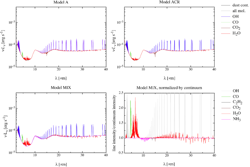
Figure 9.— LTE line spectra for model A, model ACR and model MIX for an observer at inclination $i=0$. For model MIX, we also show the spectrum normalized by the continuum flux in the lower right panel (for a better illustration, the color coding in the normalized spectrum is different from the other spectra and listed in lower right legend).

The abundance profile of acetylene can be explained as follows: in model MIX, its abundance is increased between $1$ and $10\,\mathrm{AU}$. Further inside, the diffusion leads to a depletion of C₂H₂. In model ACR, C₂H₂ is increased between $2$ and $10\,\mathrm{AU}$ and decreased further inside, similar to CO₂. Since the overall abundance of C₂H₂ is low and since it is located below the transition region, the absorption lines are negligibly small in the spectra of the disks in model A and model ACR. The stark increase in C₂H₂ in model MIX leads to a weak absorption feature seen at $13$–$13.5\micron$ (Figure 9).

3.4. Theory versus observations

We refer to the observations of the protoplanetary disks of AA Tauri (Carr & Najita, 2008), DR Tauri and AS 205 (Salyk et al., 2008). AA Tauri is a classical T Tauri star with mass $0.8M_{\odot}$, accretion rate $10^{-8}M_{\odot}\mathrm{yr}^{-1}$ and inclination $75^{\circ}$ (Bouvier et al., 1999). Carr & Najita (2008) observed the disk around AA Tauri with the Infrared Spectrograph (IRS) on the Spitzer Space Telescope over the wavelength range of $9.9$–$37.2\micron$. They found a rich spectrum of molecular emission lines dominated by rotational transitions of H₂O and OH. Between $10$ and $15\micron$, they detected ro-vibrational emission bands of C₂H₂, HCN and CO₂, plus the atomic [Ne II] transition at $12.8\micron$. Fundamental ro-vibrational emission bands of CO have been detected in Keck/NIRSPEC observations between $3$ and $5\micron$. Fitting model spectra to the observations, Carr & Najita (2008) derive a high column density for these species and characteristic emission radii in the inner disk ($s<2.5\,\mathrm{AU}$).

DR Tauri and AS 205, both classical T Tauri stars, have been observed with IRS on Spitzer and with Keck/NIRSPEC by Salyk et al. (2008). DR Tauri has a mass of $0.76M_{\odot}$ and a variable accretion rate of $[0.3$–$79]\cdot 10^{-7}M_{\odot}\mathrm{yr}^{-1}$, much higher than in our model or that observed in AA Tauri. AS 205 is the primary component of a triple system with mass $1.2M_{\odot}$ and accretion rate $7.2\cdot 10^{-7}M_{\odot}\mathrm{yr}^{-1}$. The inclinations are $67^{\circ}$ for DR Tauri and $47^{\circ}$ for AS 205A, respectively. Both systems show a large number of transitional emission lines from water and require high temperatures and column densities to explain this emission, similar to AA Tauri. Further, CO, OH and CO₂ are required to fit the observed spectra in the near- to mid-infrared. In the following, we discuss how our models relate to, and compare with, these observational results.

The calculated spectra for our models show emission and absorption features different from the observed spectra (Figure 9). Firstly, the molecular line emission in our models is dominated by rotational transitions of OH. Weak emission from H₂O is detected in model MIX. In model ACR and in model A, water is found mainly in absorption. Model WND leads to results similar to model A due to the limitations of our disk model. These models make use of the simple H₂ formation rates on grains, Eq. (2). Model B, which accounts for the enhanced H₂ formation rates on grains, Eq. (4), leads to huge emission lines from OH and H₂O. The near-infrared emission bands of CO at $5\micron$ are reproduced in model A, model MIX and also in model ACR.

The modeled line intensities depend strongly on the gas temperature and molecular abundances profiles, i. e., the detailed thermal balance and the chemistry. It is therefore more favorable to compare the molecular column densities from our model calculations to the observed ones. In the inner disk, the observed column densities and abundance ratios are derived from the photodestruction layer and the warm molecular layer, i. e., from the disk surface down to an optical depth of about unity. The total molecular column densities in our model are mainly determined by the dense midplane layers and are therefore larger by orders of magnitude and not comparable to the observed column densities. Thus, we calculate the column densities of the observed species from the disk surface down to a continuum optical depth of unity at each wavelength and compare them to the observations (Figure 10). At $s=1.3\,\mathrm{AU}$ and wavelengths $\lambda=\{5,10,20,40\}\,\micron$, the disk becomes optically thick at $z/s=\{0.14,0.15,0.14,0.11\}$, respectively. For the unusually strong OH lines, a continuum optical depth of unity corresponds to a maximum optical depth of $\tau\sim 20$ (see discussion below for large discrepancy between the models and the observations of OH lines). For all other molecules, the maximum optical depth of the lines is $\tau\sim 2$.

If we compare the H₂O and CO column densities of the upper layers at disk radius $1.3\,\mathrm{AU}$, we find an abundance ratio of $0.02$ for model A and model ACR, while model MIX shows an abundance ratio of $0.18$. Carr & Najita (2008) derive an abundance ratio of H₂O to CO of $1.3$, while Salyk et al. (2008) find water to be less abundant than carbon monoxide with an abundance ratio for H₂O to CO of $0.1$ for both systems. Note that Carr & Najita (2008) calculate the abundance ratio for different radii of the H₂O and CO column densities ($2.1\,\mathrm{AU}$ and $0.7\,\mathrm{AU}$), while Salyk et al. (2008) obtain their results for the same radius ($3\,\mathrm{AU}$). It is important to note that the observed systems differ from our model in their central objects, disk masses, inclination angles and accretion rates, with AA Tauri being the closest match. Further, the derived column densities in Carr & Najita (2008) and Salyk et al. (2008) contain considerable uncertainties in their values and their characteristic radii.

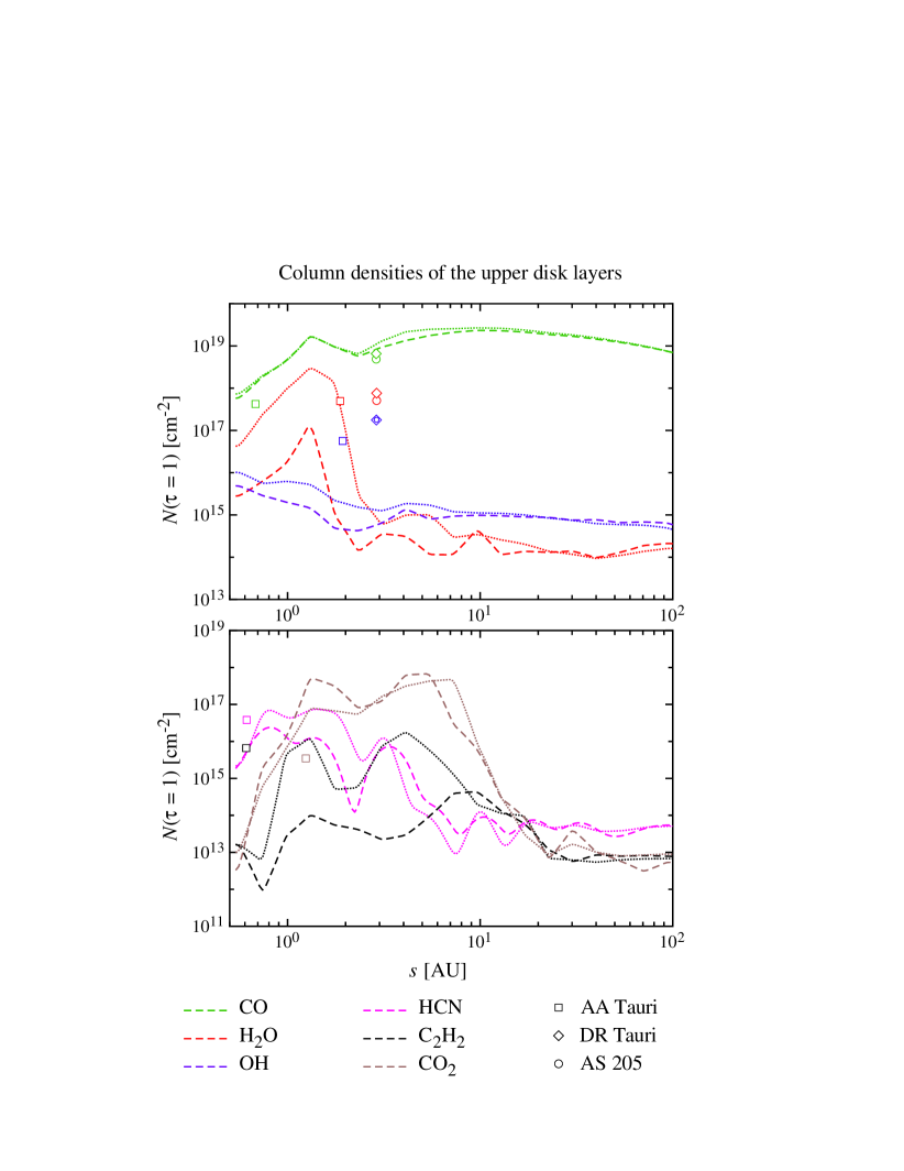
Figure 10.— Column densities of the gas-phase species in the upper layers in model A (dashed) and model MIX (dotted). The derived column densities for AA Tauri, DR Tauri and AS 205 are indicated at their characteristic radii (Carr & Najita, 2008; Salyk et al., 2008).

The resulting column densities of the upper disk layers are displayed in Figure 10 for model A and for model MIX only, since it leads to the largest changes in the vertical distribution of the chemical species. In model MIX, the H₂O to CO abundance ratio is of the order of $0.2$ inside the snow line, while in model A, it is reduced by at least a factor of $10$. Model MIX reproduces the H₂O abundance in AA Tauri at a radius of $2.1\,\mathrm{AU}$. In the case of DR Tauri and AS 205, the central star is more luminous than in AA Tauri and in our model, hence, the snow line is located further outwards and gas-phase H₂O remains abundant with derived column densities of the same order as in our model or in AA Tauri at radii of $2\,\mathrm{AU}$. The modeled CO abundances agree with the observations for both models. Both models fail to reproduce the high OH abundances, although the calculated line emission is much stronger than that of the observations. This adds further support to the call for non-LTE spectral calculations and gas temperature profile calculations accounting for dust-grain settling and grain growth (c. f., Section 3.1). Since the binding energy of OH on dust grains is low and considering it is robust against UV radiation, efficient turbulent mixing can increase the abundances in the upper layers of the disk (c. f., Figure 10).

CO₂ is found in absorption instead of in emission in model A, model ACR and model MIX. The absorption is strongest in model ACR and weakest in model MIX. Contrary to this, the observations detect CO₂ in emission at a characteristic radius of $1.2\,\mathrm{AU}$ in AA Tauri. It is also detected in emission towards DR Tauri and AS 205 (with large uncertainties on the column densities and the emission radii). The column densities derived from the observations of AA Tauri are lower than in model A and model MIX, although the latter one gives a better fit. Since CO₂ is destroyed quickly in the upper layers of the disk, stronger mixing will lead to lower CO₂ abundances.

HCN is detected in weak emission in AA Tauri and a number of other sources (see, for example, Pontoppidan et al., 2010), but not detected in our modeled spectra. The column density in AA Tauri is slightly higher than in our models, and model MIX again gives a better fit. Turbulent mixing increases the column density in the upper layers, although the total column density is reduced. Stronger mixing will help to improve the fit of the model calculations to the observations.

In the case of C₂H₂, the characteristic radius in AA Tauri could not be determined and was set to that derived for HCN. Assuming that the C₂H₂ emission is located at larger radii (e. g., $1\,\mathrm{AU}$ instead of $0.6\,\mathrm{AU}$), model MIX fits the observed column density, while model A predicts much lower values. Adversely, the spectrum of model MIX shows C₂H₂ in weak absorption instead of emission. From the previous discussion in Sections 3.2 and 3.3, we can assume that stronger turbulence will transport C₂H₂ higher up in the disk, leading to emission instead of absorption signatures.

The abundances of NH₃ are enhanced in model MIX, leading to absorption signatures in the spectrum between $8$ and $13\micron$. To date, there has been no published detection of ammonia from protoplanetary disks, but NH₃ has been found in absorption towards the hot core associated with the massive protostar NGC 7538 IRS 1 (Knez et al., 2009), using the Texas Echelon Cross Echelle Spectrograph (TEXES). Observing NH₃ emission from disks with high resolution and high sensitivity will allow us to draw important conclusions on the efficiency of turbulent mixing in protoplanetary disks.

Taking into account the model uncertainties, e. g. the H₂ formation rates on grains, the gas temperature profiles (which are related to the dust model adopted, e. g., to the dust growth and settling), as well as the uncertainties in deriving molecular column densities and characteristic radii from the observations, further investigations are needed to strengthen the significance of our results.

In addition, the observed objects have inclination angles of $67^{\circ}$ for DR Tauri and $47^{\circ}$ for AS 205A, while our theoretical spectra are calculated for a disk seen face-on. This affects the observed line emission and the derived column densities, since the chemical composition is different along the line of sight. Robust conclusions therefore require spectral calculations accounting for the different inclination angles.

4. Conclusion

We studied the chemical evolution of a steady protoplanetary disk, investigating different models for the formation rate of H₂ on dust grains and the effects of including viscous accretion, turbulent mixing and disk winds. Using our chemical results, we calculated the emergent near- and mid-infrared spectrum from the disk, including contributions from the dust continuum and molecular line emission.

Our results show that the abundances of water and the hydroxyl radical are very sensitive to the H₂ formation rates on grains, with the resulting spectra differing considerably. The enhanced H₂ formation rates of Cazaux & Tielens (2002) lead to a drastic increase in the gas-phase abundances of water and OH in the upper disk layers and to strong emission lines. We concluded that dust grain settlement towards the midplane and non-LTE calculations of the molecular line emission are required to obtain meaningful results for models using these enhanced H₂ formation rates.

We investigated the effects of physical mass transport phenomena in the radial direction by viscous accretion and in the vertical direction by diffusive turbulent mixing and disk winds. Due to the steady state assumption of the underlying protoplanetary disk model, the wind velocities are limited to impede the evaporation of the disk over its lifetime and consequently, the effects of the disk winds on the chemistry are small. On the contrary, vertical diffusive mixing has a considerable impact on the disk chemistry and increases the abundance of many observed species in the warm molecular layer of the disk. Species which are produced efficiently in a particular layer and which are stable in lower (or upper) layers can experience a significant enhancement due to the diffusive motion. Including the radial accretion flow in the chemical network calculation leads to large changes in the chemical composition of the disk, particularly in the cold and dense midplane layer. The effect of the accretion flow on a particular species depends on the accretion timescale and the formation and destruction timescales of that species. For example, inside $10\,\mathrm{AU}$, the gas-phase water abundances are not overly affected by the accretion flow, while ammonia is greatly enhanced and methanol, greatly depleted.

Since the accretion flow affects mainly the midplane layers, the infrared molecular line emission is basically unchanged. Contrarily, turbulent mixing alters the chemical composition of the warm molecular layer, where the molecular line emission is generated. We thus contrasted two models with and without turbulent mixing to observations of protoplanetary disks around classical T Tauri stars. We compared the modeled disk spectra and column densities of the upper layers of the disk to the observed spectra and the derived column densities.

In summary, a model with turbulent mixing reproduces the observations of AA Tauri, DR Tauri and AS 205 better than a model without mixing, although the discussion of the column densities in the upper layers and of the spectra suggests a more efficient vertical mass transport mechanism. In the models considered here, turbulent mixing provides an efficient way of transporting material from the midplane into the transition layer. Due to the constant mixing velocity in each vertical column, the turbulent timescales become longer than the chemical timescales at larger distances from the midplane. But these are the layers where the disk winds studied by Suzuki & Inutsuka (2009) become most effective (the transition layer coincides roughly with $1.5$ disk scale heights) and drive large-scale channel flows. Hence, a combination of turbulence in the cold midplane layers and disk winds in the transition layer, both generated by the magneto-rotational instability, might account for the observations better than turbulent mixing or disk winds alone. In the latter case, the steady state assumption would have to be abandoned to allow for stronger disk winds.

An interesting aspect for future studies will be the combination of radial and vertical transport processes. In this work, we showed that the radial accretion flow alters predominantly the midplane abundances, while turbulent mixing affects the midplane and warm molecular layers. We therefore expect that a combination of radial and vertical motion will have a strong impact on the chemical abundances in the molecular layer, which will be reflected in the emission line spectrum.

Appendix A A. Physicochemical interactions – numerics

Modeling the physical mass transport phenomena in combination with calculating the chemical evolution is the key aspect of this study. Here, we discuss in detail the numerical techniques used to compute the chemistry accounting for transport mechanisms in relation to the grid of our protoplanetary disk model.

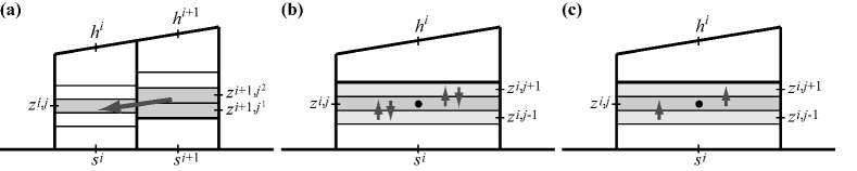
Figure 11.— Schematic view of (a) accretion, (b) mixing and (c) wind modeling in our model.

The general expression for the rate of change in the abundance of gas-phase species $k$ in grid cell $(i,j)$ at radius $s^{i}$ and vertical distance $z^{j}$ from the midplane is given by

$$\dot{n}_{k}^{i,j}=\frac{\Delta n_{k}^{i,j}}{\Delta t}=P_{k}^{i,j}-L_{k}^{i,j}-\dot{n}_{k\,\mathrm{ice}}^{i,j}+\dot{n}_{k,\,\mathrm{acc/mix/wind}}^{i,j}\,,$$ (A1)

where $P_{k}$ and $L_{k}$ denote the production and loss terms due to gas-phase chemical reactions, $\dot{n}_{k\,\mathrm{ice}}$ the adsorption/desorption rate ($>0$ for net freeze-out, $<0$ for net evaporation) and $\dot{n}_{k,\,\mathrm{acc/mix/wind}}$ the rates arising from mass transport due to accretion, mixing or disk winds. In the case of molecular hydrogen, an additional (positive) term $\dot{n}_{\mathrm{H}_{2}}$ is added to the right-hand side to account for the H₂ formation on grains. Accordingly, in the case of atomic hydrogen, an additional term $-2\dot{n}_{\mathrm{H}_{2}}$ is required.

A.1. A.1 Radial transport by viscous accretion

We assume that inward accretion occurs along constant streamlines $z/h$. (see Figure 11(a) for an illustration of the coupling between the grid cells at different radii). The net accretion rate along constant streamlines is given in Equation (15), where the differentiation with respect to $l$ needs to be translated into a differentiation with respect to $s$. Accordingly, on the discrete grid of the disk model, the net accretion rate for cell $(i,j)$ can be expressed as

$$\dot{n}_{k,\,\mathrm{acc}}^{i,j}=\frac{\bar{v}_{s}^{i,i+1}}{\Delta s^{i}}\left\{-n_{k}^{i,j}+\frac{\tilde{\rho}^{i+1,j^{1}\!,j^{2}\!}}{\rho^{i,j}}\tilde{n}_{k}^{i+1,j^{1}\!,j^{2}\!}\right\}$$ (A2)

where $\tilde{\rho}$ and $\tilde{n}$ represent the average mass and number density of the outer grid cells, weighed by their relative mass transfer into cell $(i,j)$. The accretion velocity $\bar{v}_{s}^{i,i+1}$ is evaluated at the interface between the grid cells $i$ and $i+1$ and is introduced to improve the accuracy of the finite calculation. The additional factor $\tilde{\rho}^{i+1,j^{1}\!,j^{2}\!}/\rho^{i,j}$ arises from the requirement of mass conservation. In the context of a steady disk model, all variables except $n_{k}^{i,j}$ and $\tilde{n}_{k}^{i+1,j^{1}\!,j^{2}}$ are constant with time.

A.2. A.2 Vertical transport by turbulent mixing

Figure 11(b) demonstrates the grid-cell mass transfer by turbulent mixing in the diffusion-type model. Starting from Equation (18), we replace the differentials by finite differences over the vertical extent $\Delta z$ of the grid cells. Additionally, we introduce mean densities $\bar{\rho}$ and velocities $\bar{v}$ at the interface of the grid cells as before. The exchange rates of species $k$ between grid cell $(i,j)$ and the adjacent grid cells $(i,j-1)$ and $(i,j+1)$ then become

$$\dot{n}_{k,\,\mathrm{mix}}^{i,j}=\frac{\bar{\rho}^{i,j-1,j}}{\rho^{i,j-1}}\cdot\frac{\bar{v}_{z}^{i,j-1,j}}{\Delta z^{i,j}}\cdot\left(n_{k}^{i,j-1}-\frac{\rho^{i,j-1}}{\rho^{i,j}}\,n_{k}^{i,j}\right)+\frac{\bar{\rho}^{i,j,j+1}}{\rho^{i,j}}\cdot\frac{\bar{v}_{z}^{i,j,j+1}}{\Delta z^{i,j}}\cdot\left(\frac{\rho^{i,j}}{\rho^{i,j+1}}\,n_{k}^{i,j+1}-n_{k}^{i,j}\right).$$ (A3)

A.3. A.3 Vertical transport by disk winds

The model of the upward disk wind is shown in Figure 11(c). In the finite case, the differential equation for the wind rate (Equation (20)) of grid cell $(i,j)$ translates into

$$\dot{n}_{k,\,\mathrm{wind}}^{i,j}=\frac{v_{z}^{i,j-1,j}}{{\Delta z}^{i,j}}\cdot n_{k}^{i,j-1}-\frac{v_{z}^{i,j,j+1}}{{\Delta z}^{i,j}}n_{k}^{i,j}\,.$$ (A4)

In both the wind and the mixing scenarios, the only variable changing with time is $n_{k}$.

References

- Aikawa et al. (1996) Aikawa, Y., Miyama, S. M., Nakano, T., & Umebayashi, T. 1996, ApJ, 467, 684
- Aikawa et al. (1999) Aikawa, Y., Umebayashi, T., Nakano, T., & Miyama, S. M. 1999, ApJ, 519, 705
- Aikawa et al. (2002) Aikawa, Y., van Zadelhoff, G. J., van Dishoeck, E. F., & Herbst, E. 2002, A&A, 386, 622
- Aikawa & Nomura (2006) Aikawa, Y., & Nomura H. 2006, ApJ, 642, 1152
- Armitage (2007) Armitage, P. J. 2007, ApJ, 665, 1381
- Beckwith et al. (1990) Beckwith, S. V. W., Sargent, A. I., Chini, R. S., & Guesten, R. 1990, AJ, 99, 924
- Blandford & Payne (1982) Blandford, R. D., Payne, D. G. 1982, MNRAS, 199, 883
- Brittain et al. (2009) Brittain, S. D., Najita, J. R., & Carr, J. S. 2009, ApJ, 702, 85
- Bouvier et al. (1999) Bouvier, J. et al. 1999, A&A, 349, 619
- Brown & Bolina (2007) Brown, W. A., & Bolina, A. S. 2007, MNRAS, 374, 1006
- Carmona et al. (2007) Carmona, A., van den Ancker, M. E., Henning, Th., Goto, M., Fedele, D., & Stecklum, B. 2007, A&A, 476, 853
- Carmona (2010) Carmona, A. 2010, in Earth, Moon, and Planets, ed. G. B. Valsecchi & M. S. Gudipati, 71
- Carr (2007) Carr, J. S. 2007, in IAU Symp. 243, Star-Disk Interaction in Young Stars, ed. J. Bouvier & I. Appenzeller, 135
- Carr & Najita (2008) Carr, J. S., & Najita, J. R. 2008, Science, 319, 1504
- Cazaux & Tielens (2002) Cazaux, S., & Tielens, A. G. G. M. 2002, ApJ, 575, L29
- Charnley (1997) Charnley, S. B. 1997, ApJ, 481, 396
- Courant et al. (1928) Courant, R., Friedrichs K., & Lewy, H. 1928, Mathematische Annalen, 100, 32
- Dominik et al. (2007) Dominik, C., Blum, J., Cuzzi, J. N., Wurm, G. 2007, in Protostars and Planets V, ed. B. Reipurth, D. Jewitt, & K. Keil, 783
- Draine (1978) Draine, B. T. 1978, ApJS, 36, 595
- Duley & Williams (1984) Duley, W. W., & Williams, D. A. 1984, Interstellar chemistry (London: Academic Press)
- Dullemond & Turolla (2000) Dullemond, C. P., & Turolla, R. 2000, A&A, 360, 1187
- Dullemond et al. (2002) Dullemond, C. P., van Zadelhoff, G. J., & Natta, A. 2002, A&A, 389, 464
- Dutrey et al. (2007) Dutrey, A., Guilloteau, S., & Ho, P. 2007, in Protostars and Planets V, ed. B. Reipurth, D. Jewitt, & K. Keil, 495
- Fogel et al. (2011) Fogel, J. K. J., Bethell, T. J., Bergin, E. A., Calvet, N., & Semenov, D. 2011, ApJ, accepted for publication (astro-ph.1011.0446)
- Geers et al. (2006) Geers, V. C. et al. 2006, A&A, 459, 545
- Gibb et al. (2007) Gibb, E. L., Van Brunt, K. A., Brittain, S. D., & Rettig, T. W. 2007, ApJ, 660, 1572
- Glassgold et al. (2004) Glassgold, A. E., Najita, J., & Igea, J., 2004, ApJ, 615, 972
- Glassgold et al. (2009) Glassgold, A. E., Meijerink, R., & Najita, J. R. 2009, ApJ, 701, 142
- Gorti & Hollenbach (2004) Gorti, U., & Hollenbach, D. 2004, ApJ, 613, 424
- Gould & Salpeter (1963) Gould, R. J., & Salpeter, E. E. 1963, ApJ, 138, 393
- Habert et al. (2006) Habart, E., Natta, A., Testi, L., & Carbillet, M. 2006, A&A, 449, 106
- Haisch et al. (2001) Haisch, Jr., K. E., Lada, E. A., & Lada, C. J. 2001,ApJ, 553, L153
- Haisch et al. (2006) Haisch, Jr., K. E., Barsony, M., Ressler, M. E., & Greene, T. P. 2006, AJ, 132, 2675
- Hasegawa & Herbst (1993) Hasegawa, T. I., & Herbst, E. 1993, MNRAS, 261, 83
- Hatchell et al. (1998) Hatchell, J., Thompson, M. A., Millar, T. J., & MacDonald, G. H. 1998, A&A, 338, 713
- Hollenbach & McKee (1979) Hollenbach, D., & McKee, C. F. 1979, ApJS, 41, 555
- Hollenbach & Salpeter (1971) Hollenbach, D., & Salpeter, E. E. 1971, ApJ, 163, 155
- Hogerheijde & van der Tak (2000) Hogerheijde, M., & van der Tak, F. 2000, A&A, 362, 697
- Ilgner et al. (2004) Ilgner, M., Henning, Th., Markwick, A. J., & Millar, T. J. 2004, A&A, 415, 643
- Jonkheid et al. (2004) Jonkheid, B., Faas, F. G. A., van Zadelhoff, G.-J., & van Dishoeck, E. F. 2004, A&A, 428, 511
- Kamp & Dullemond (2004) Kamp, I., & Dullemond, C. P. 2004, ApJ, 615, 991
- Knez et al. (2009) Knez, C., Lacy, J. H., Evans, N. J., van Dishoeck, E. F., & Richter M. J. 2009, ApJ, 696, 471
- Lada & Willking (1984) Lada, C. J., & Wilking, B. A. 1984, ApJ, 287, 610
- Lahuis et al. (2006) Lahuis, F. et al. 2006, ApJ, 636, L145
- Markwick et al. (2002) Markwick, A. J., Ilgner, M., Millar, T. J., & Henning, Th. 2002, A&A, 385, 632
- Meijerink et al. (2009) Meijerink, R., Pontoppidan, K. M., Blake, G. A., Poelman, D. R., & Dullemond, C. P. 2009, ApJ, 704, 1471
- Millar et al. (1997) Millar, T. J., MacDonald, G. H., & Gibb, A. G. 1997, A&A, 325, 1163
- Najita et al. (2007) Naijta, J. R., Carr, J. S., Glassgold, A. E., & Valenti, J. A. 2007, in Protostars and Planets V, ed. B. Reipurth, D. Jewitt, & K. Keil, 507
- Natta (2007) Natta, A., Testi, L., Calvet, N., Henning, Th., Waters, R., & Wilner, D. 2007, in Protostars and Planets V, ed. B. Reipurth, D. Jewitt, & K. Keil, 767
- Nomura (2002) Nomura, H. 2002, ApJ, 567, 587
- Nomura & Millar (2005) Nomura, H., & Millar T. J. 2005, A&A, 438, 923
- Nomura et al. (2007) Nomura, H., Aikawa, Y., Tsujimoto, M., Nakagawa, Y., & Millar, T. J. 2007, ApJ, 661, 334
- Nomura et al. (2009) Nomura, H., Aikawa, Y., Nakagawa, Y., & Millar, T. J. 2009, A&A, 495, 183
- Ossenkopf & Henning (1994) Ossenkopf, V., & Henning, Th. 1994, A&A, 291, 943
- Pontoppidan et al. (2008) Pontoppidan, K. M., Blake, G. A., van Dishoeck, E. F., Smette, A., Ireland, M. J., & Brown, J. 2008, ApJ, 684, 1323
- Pontoppidan et al. (2010) Pontoppidan, K. M., Salyk, C., Blake, G. A., Meijerink, R., Carr, J. S., & Najita J. R. 2010, ApJ, 720, 887
- Pringle (1981) Pringle, J. E. 1981, ARA&A, 19, 137
- Qi et al. (2006) Qi, C., Wilner, D. J., Calvet, N., Bourke, T. L., Blake, G. A.; Hogerheijde, M. R., Ho, P. T. P., & Bergin, E. 2006, ApJ, 636, L157
- Rodgers & Charnley (2001) Rodgers, S. D., & Charnley, S. B. 2001, ApJ, 546, 324
- Rothman et al. (2005) Rothman, L. S. et al. 2005, JQSRT, 96, 139
- Salyk et al. (2008) Salyk, C., Pontoppidan, K. M., Blake, G. A., Lahuis, F., van Dishoeck, E. F., & Evans, N. J. 2008, ApJ, 676, L49
- Semenov et al. (2006) Semenov, D., Wiebe, D., & Henning, Th. 2006, ApJ, 647, L57
- Sandford & Allamondola (1988) Sandford, S. A., & Allamondola, L. J. 1988, Icarus, 76, 201
- Sandford & Allamondola (1990) Sandford, S. A., & Allamondola, L. J. 1990, Icarus, 87, 188
- Sandford & Allamondola (1993) Sandford, S. A., & Allamondola, L. J. 1993, ApJ, 417, 815
- Shakura & Sunyaev (1973) Shakura, N. I., & Sunyaev, R. A. 1973, A&A, 24, 337
- Shu et al. (1993) Shu, F., Najita, J., Ostriker, E., Wilkin, F., Ruden, S., & Lizano, S. 1993, ApJ, 429, 781
- Shu et al. (1994) Shu, F., Johnstone, D., & Hollenbach, D. 1994, Icarus, 106, 92
- Suzuki & Inutsuka (2009) Suzuki, T. K., & Inutsuka, S. 2009, ApJ, 691, L49
- van der Plas et al. (2009) van der Plas, G., van den Ancker, M. E., Acke, B., Carmona, A., Dominik, C., Fedele, D., & Waters, L. B. F. M. 2009, A&A, 500, 1137
- van Dishoeck & Black (1982) van Dishoeck, E. F. & Black, J. H. 1982, ApJ, 258, 533
- Walsh et al. (2010) Walsh, C., Millar, T. J., & Nomura, H. 2010, ApJ, 722, 1607
- Watson et al. (2007) Watson, A. M., Stapefeldt, K. R., Wood, K., & Ménard, F. 2007, in Protostar and Planets V, ed. B. Reipurth, D. Jewitt, & K. Keil, 523
- Weingartner & Draine (2001a) Weingartner, J. C., & Draine, B. T. 2001, ApJ, 548, 296
- Weingartner & Draine (2001b) Weingartner, J. C., & Draine, B. T. 2001, ApJS, 134, 263
- Westley et al. (1995) Westley, M. S., Baragiola, R. A., Johnson, R. E., & Baratta, G. A 1995, Planet. Space Sci., 43, 1311
- Willacy et al. (2006) Willacy, K., Langer, W., Allen, M., & Bryden, G., 2006, ApJ, 644, 1202
- Willacy (2007) Willacy, K. 2007, ApJ, 660, 441
- Wolk et al. (2005) Wolk, S. J., Harnden, F. R., Flaccomio, E., Micela, G., Favata, F., Shang, H., & Feigelson, E. D. 2005, ApJS, 160, 423
- Woitke et al. (2009a) Woitke, P., Kamp, I., & Thi, W.-F. 2009, A&A, 501, 383
- Woitke et al. (2009b) Woitke, P., Thi, W.-F., Kamp, I., & Hogerheijde, M. R. 2009, A&A, 501, L5
- Woodall et al. (2007) Woodall, J.. Agúndez, M., Markwick-Kemper, A. J., & Millar, T. J. 2007, A&A, 466, 1197
- Woods & Willacy (2009) Woods, P. M., & Willacy, K. 2009, ApJ, 693, 1360
- Yamamoto et al. (1983) Yamamoto, T., Nakagawa, N., & Fukui, Y. 1983, A&A, 122, 171