Non-equilibrium electromagnetic fluctuations: Heat transfer and interactions

Abstract

The Casimir force between arbitrary objects in equilibrium is related to scattering from individual bodies. We extend this approach to heat transfer and Casimir forces in non-equilibrium cases where each body, and the environment, is at a different temperature. The formalism tracks the radiation from each body and its scatterings by the other objects. We discuss the radiation from a cylinder, emphasizing its polarized nature, and obtain the heat transfer between a sphere and a plate, demonstrating the validity of proximity transfer approximation at close separations and arbitrary temperatures.

The electromagnetic field in the space around bodies is stochastic due to quantum and thermal fluctuations. The basic formalism of Fluctuational Electrodynamics (FE), was set out over 60 years ago by Rytov Rytov et al. (1989), and has been applied extensively since to diverse problems in radiative heat transfer Polder and Van Hove (1971); Modest (2003) and Casimir forces Lifshitz (1956). FE starts with casting the current fluctuations in each body in terms of its dielectric properties, and proceeds to compute the resulting electromagnetic field. The improved precision of measurements of force and heat transfer at sub-micron scale have provided renewed incentive to examine FE for objects at different temperatures Bordag et al. (2009). In particular, when the size or separation of the objects is comparable to, or smaller than, the thermal wavelength (around 8 micron at room temperature), heat radiation and transfer will differ from the predictions of the Stefan-Boltzmann law: The considerably larger near-field heat transfer, due to tunneling of evanescent waves, has been verified experimentally Sheng et al. (2009); et. al. (2009). Theoretical computations of heat transfer were only recently extended from two parallel plates Polder and Van Hove (1971) or dipoles Volokitin and Persson (2001) to two spheres Narayanaswamy and Chen (2008). The radiation of single spheres and plates has been studied by many authors Kattawar and Eisner (1970); Bohren and Huffmann (2004). For a cylinder, the emissivity restricted to waves traveling perpendicular to its axis has been addressed et. al. (2009). There are also recent computations of the non-equilibrium Casimir force between objects at different temperatures, for parallel plates Antezza et al. (2008), modulated plates Bimonte (2009), as well as a plate and an atom Antezza et al. (2005). The limitation of these results to simple shapes and arrangements points out the need for approaches capable of handling more complex situations.

Here, we derive a formalism for computing heat transfer and Casimir forces for arbitrary objects (compact or not) maintained at different temperatures. Generalizing previous work on Casimir forces in equilibrium, our approach enables systematic description of FE of a collection of objects in terms of their individual scattering properties. For the non-equilibrium Casimir force, we can investigate interactions between compact objects where, unlike previous studies Antezza et al. (2005, 2008); Bimonte (2009), the effect of a third temperature (of the environment) has to be taken into account. In terms of new applications, we derive the heat radiation of a cylinder which is of interest for heated wires or carbon nanotubes Fan et al. (2009). We also study the heat transfer between a sphere and a plate, the only geometry for which near field heat transfer has been measured Sheng et al. (2009); et. al. (2009).

Consider an arrangement of $N$ objects labelled as $\alpha=1\dots N$, in vacuum at constant temperatures $\{T_{\alpha}\}$, and embedded in an environment at temperature $T_{env}$. In this non-equilibrium stationary state, each object is assumed to be at local equilibrium with current fluctuations obeying the fluctuation-dissipation theorem (FDT). In the following, we derive the autocorrelation function $C$ of the electric field $\mathbf{E}$ at frequency $\omega$ at points $\mathbf{r}$ and $\mathbf{r}^{\prime}$ outside the objects, from which the Poynting vector for heat transfer and the Maxwell stress tensor for Casimir forces can then be extracted. In equilibrium, with $T_{\alpha}=T_{env}=T$, $C$ is related to the imaginary part of the dyadic Green’s function $G_{ij}$ by Rytov et al. (1989); Eckhardt (1984),

$$C_{ij}^{eq}(T) \equiv\left\langle E_{i}(\omega;\mathbf{r})E_{j}^{*}(\omega;\mathbf{r}^{\prime})\right\rangle^{eq}$$

$$=\left[a_{T}(\omega)+a_{0}(\omega)\right]\frac{c^{2}}{\omega^{2}}\operatorname{Im}G_{ij}(\omega;\mathbf{r},\mathbf{r}^{\prime}),$$ (1)

where $a_{T}(\omega)\equiv\frac{\omega^{4}\hbar(4\pi)^{2}}{c^{4}}(\exp[\hbar\omega/k_{B}T]-1)^{-1}$ is proportional to the occupation number of all oscillators of frequency $\omega$, $c$ is the speed of light, and $\hbar$ is Planck’s constant. Zero point fluctuations which contribute $a_{0}(\omega)\equiv\frac{\omega^{4}\hbar(4\pi)^{2}}{2c^{4}}$ play no role in our discussion. We shall henceforth employ the operator notation $\mathbb{G}\equiv G_{ij}(\omega;\mathbf{r},\mathbf{r}^{\prime})$. Since $\operatorname{Im}\mathbb{G}=-\mathbb{G}\operatorname{Im}\mathbb{G}^{-1}\mathbb{G}^{*}$, and using the identity Eckhardt (1984) $\sum_{\alpha}\operatorname{Im}\varepsilon_{\alpha}\mathbb{I}=-\frac{c^{2}}{\omega^{2}}\operatorname{Im}(\mathbb{G}^{-1}-\mathbb{G}_{0}^{-1})$, where $\varepsilon_{\alpha}$ is the complex dielectric function of object $\alpha$ and $\mathbb{G}_{0}$ is the Green’s function of free space, we obtain

$$C^{eq}(T) =C_{0}+\sum_{\alpha}C_{\alpha}^{sc}(T)-a_{T}(\omega)\frac{c^{2}}{\omega^{2}}\mathbb{G}\operatorname{Im}\mathbb{G}_{0}^{-1}\mathbb{G}^{*},$$

$$C_{\alpha}^{sc}(T) =a_{T}(\omega)\mathbb{G}\operatorname{Im}\varepsilon_{\alpha}\mathbb{G}^{*},$$ (2)

where $C_{0}=a_{0}(\omega)\frac{c^{2}}{\omega^{2}}\operatorname{Im}\mathbb{G}$ is the zero point term. The finite temperature contribution is thus a sum of $N+1$ terms: Each $C_{\alpha}^{sc}(T)$ contains an implicit integral over sources within $\alpha$ and is identified with the field sourced by this object Rytov et al. (1989); the scattering of this radiation by all other objects is accounted for by multiplying $\operatorname{Im}\varepsilon_{\alpha}$ on both sides with the full Green’s function. The last term in Eq. (Non-equilibrium electromagnetic fluctuations: Heat transfer and interactions), $C^{env}(T)=-a_{T}(\omega)\frac{c^{2}}{\omega^{2}}\mathbb{G}\operatorname{Im}\mathbb{G}_{0}^{-1}\mathbb{G}^{*}$, is hence identified with the contribution sourced by the environment.

A key assumption of FE is that in a non-equilibrium situation, the thermal current fluctuations inside each object are described by the FDT at the corresponding local temperature, and are independent of the impinging radiation from the other objects. Having identified the different sources in Eq. (Non-equilibrium electromagnetic fluctuations: Heat transfer and interactions), we can change their temperatures to arrive at the desired non-equilibrium generalization

$$C^{neq}(T_{env},\{T_{\alpha}\})=C_{0}+\sum_{\alpha}C_{\alpha}^{sc}(T_{\alpha})+C^{env}(T_{env})$$

$$=C^{eq}(T_{env})+\sum_{\alpha}\left[C_{\alpha}^{sc}(T_{\alpha})-C_{\alpha}^{sc}(T_{env})\right].$$ (3)

The second form is obtained by considering the difference of $C^{neq}(T_{env},\{T_{\alpha}\})$ from $C^{eq}(T_{env})$ due to the deviations of the object temperatures $T_{\alpha}$ from $T_{env}$. This form is useful because the equilibrium correlation can be regarded as known, and the number of sources is reduced from $N+1$ to $N$. Applying the formalism, e.g., to derive Casimir forces, the first term on the r.h.s. of Eq. (3) yields the equilibrium force at temperature $T_{env}$.

The next step is to compute the radiation field of object $\alpha$ when isolated, i.e., before this field is scattered by the other objects, and with $T_{env}=0$. This is given by $C_{\alpha}(T_{\alpha})\equiv a_{T_{\alpha}}(\omega)\mathbb{G}_{\alpha}\operatorname{Im}\varepsilon_{\alpha}\mathbb{G}_{\alpha}^{*}\,$ where $\mathbb{G}_{\alpha}$ is the Green’s function of object $\alpha$ in isolation, and thus involves an implicit integration over the interior of object $\alpha$. To employ multiple scattering techniques et. al. (2009), it is considerably more convenient to express $C_{\alpha}(T_{\alpha})$ in terms of the T-operator or scattering amplitude $\mathbb{T}_{\alpha}$ of the object. In equilibrium, the electric field correlator for the isolated object $C_{\alpha}^{eq}(T_{\alpha})=a_{T_{\alpha}}(\omega)\frac{c^{2}}{\omega^{2}}\operatorname{Im}\mathbb{G}_{\alpha}$, contains radiation sourced (i) by the environment and (ii) by the object itself. The latter can be obtained by subtracting the contribution from the environment, which can be regarded as an additional material with $\varepsilon_{env}\to 1$, occupying the space complimentary to $\alpha$ Eckhardt (1984). Towards this calculation, we introduce a Green’s function $\tilde{\mathbb{G}}_{\alpha}$ with $\varepsilon_{\alpha}$ inside object $\alpha$ and $\varepsilon_{env}$ outside,

$$C_{\alpha}(T_{\alpha}) = C_{\alpha}^{eq}(T_{\alpha})-C_{\alpha}^{env}(T_{\alpha}),$$ (4)

$$C_{\alpha}^{env}(T_{\alpha}) = a_{T_{\alpha}}(\omega)\lim_{{\varepsilon_{env}}\to 1}\tilde{\mathbb{G}}_{\alpha}\operatorname{Im}{\varepsilon_{env}}~{}\tilde{\mathbb{G}}^{*}_{\alpha}.$$

Note that all sources for $C_{\alpha}^{env}(T_{\alpha})$ are outside object $\alpha$, and none of the Green’s functions appearing in Eq. (4) contain points inside the object, which can thus be written in terms of $\mathbb{T}_{\alpha}$ as $\mathbb{G}_{\alpha}=\mathbb{G}_{0}-\mathbb{G}_{0}\mathbb{T}_{\alpha}\mathbb{G}_{0}$ et. al. (2009) ($\tilde{\mathbb{G}}_{\alpha}$ is a simple modification of $\mathbb{G}_{\alpha}$ as a finite $\varepsilon_{env}-1$ only changes the external speed of light). For computing the energy radiated by object $\alpha$, one does not have to find $C_{\alpha}^{eq}(T_{\alpha})$: As a consequence of detailed balance, it does not contribute to the Poynting vector.

Finally, to compute $C_{\alpha}^{sc}(T_{\alpha})$ in Eq. (3), we need to account for scattering of the radiation emerging from $\alpha$, by all other objects collectively designated by $\beta$. Denoting their total T-operator by $\mathbb{T}_{\beta}$, by use of the Lippmann-Schwinger equation et. al. (2009), we arrive at the final form

$$C_{\alpha}^{sc}(T_{\alpha}) = \mathbb{O}_{\alpha,\beta}\,C_{\alpha}(T_{\alpha})\,\mathbb{O}_{\alpha,\beta}^{\dagger}\,,\quad{\rm with}\,$$ (5)

$$\mathbb{O}_{\alpha,\beta} = (1-\mathbb{G}_{0}\mathbb{T}_{\beta})\frac{1}{1-\mathbb{G}_{0}\mathbb{T}_{\alpha}\mathbb{G}_{0}\mathbb{T}_{\beta}}\,.$$

Expanding the resolvent leads to an alternating application of $\mathbb{T}_{\beta}$ and $\mathbb{T}_{\alpha}$, corresponding to a sequence of scatterings between the objects. Equations (5) and (3) constitute our non-equilibrium formalism.

The correlator $C^{neq}$ enables computing the Poynting vector and Maxwell stress tensor, respectively given by

$$\mathbf{S}(\mathbf{r}) =\frac{c}{4\pi}\int\frac{d\omega}{(2\pi)^{2}}\left\langle\mathbf{E}(\omega,\mathbf{r})\times\mathbf{B}^{*}(\omega,\mathbf{r})\right\rangle\,,$$

$$T_{ij}(\mathbf{r}) =\int\frac{d\omega}{16\pi^{3}}\left\langle E_{i}E^{*}_{j}+B_{i}B^{*}_{j}-\frac{1}{2}\left(|E|^{2}+|B|^{2}\right)\delta_{ij}\right\rangle,$$

where the arguments $\omega$ and $\mathbf{r}$ are omitted in the lower line. The heat $H$ absorbed per unit time by object $\alpha$, and the force $F_{i}$ acting on this object in direction $i$, are then obtained by integrations of $\mathbf{S}$ and $T_{ij}$ over a surface $\sigma_{\alpha}$ enclosing only this object, as

$$H_{\alpha}=-\operatorname{Re}\oint_{\sigma_{\alpha}}\mathbf{S}\cdot\mathbf{n}_{\alpha}\,d\sigma,\,\,\,F_{i,\alpha}=\operatorname{Re}\oint_{\sigma_{\alpha}}T_{ij}n_{\alpha,j}\,d\sigma,$$ (6)

where $\mathbf{n}_{\alpha}$ is the outward normal to the surface $\sigma_{\alpha}$.

As a first application we compare heat radiations from a single object, a plate, sphere or cylinder; the only shapes amenable to analytic treatment. As formulae for heat radiation of a sphere or a plate are available in the literature Kattawar and Eisner (1970); Rytov et al. (1989), we focus on the cylinder where the corresponding result is only discussed implicitly Rytov (1959). For an infinitely long cylinder, $\mathbb{T}$ is represented in cylindrical wave functions et. al. (2009), indexed by $(n,k_{\|},P)$ where $n$ is the multipole order, $k_{\|}$ the wave vector component along the cylinder, and $P=E$ or $P=M$ the polarization. The matrix element $T^{P^{\prime}P}_{n,k_{\|}}$ describes the relative amplitude of the scattered wave of mode $(n,k_{\|},P^{\prime})$ emerging from an incoming wave $(n,k_{\|},P)$. We then find for the radiated heat of the single cylinder per length $L$,

$$\frac{|H_{c}|}{L} =-\int_{0}^{\infty}\frac{d\omega}{(2\pi)^{2}}a_{T}(\omega)\frac{c^{4}}{4\pi^{2}\omega^{3}}\sum_{P=E,M}\sum_{n=-\infty}^{\infty}$$ (7)

$$\int\limits_{-\omega/c}^{\omega/c}dk_{||}\left(\operatorname{Re}[T_{n,k_{||}}^{PP}]+|T_{n,k_{||}}^{PP}|^{2}+|T_{n,k_{||}}^{P\bar{P}}|^{2}\right),$$

where $\bar{P}=M$, if $P=E$ and vice versa. In Fig. 1, we compare the heat radiation of a plate (semi-infinite body), a sphere and a cylinder (both of radius $R$), all evaluated with optical data of silicon-dioxide (SiO₂), as used in experiments Sheng et al. (2009). The radiation is normalized to the Stefan-Boltzmann law $H=\sigma T^{4}A$, with $\sigma=\pi^{2}k_{B}^{4}/(60\hbar^{3}c^{2})$ and surface area $A$ of the object.

For thin cylinders and small spheres $H$ is proportional to the volume, while in the opposite limit, it is proportional to the surface area, reflecting a finite skin depth (absorption length) $\delta(\omega)=c/(\operatorname{Im}\sqrt{\varepsilon}\omega)$: Thermal fluctuations at frequency $\omega$ within the object emit radiation which may be re-absorbed on its way out. If $\delta\ll R$, only thermal fluctuations near the surface lead to emerging radiation, while for $\delta\gg R$, the entire volume contributes to $H$. An interesting feature of Fig. 1 is the intermediate range, where the sphere and cylinder emit more strongly than a plate of equal area, related to Mie resonances for the sphere Bohren and Huffmann (2004). For $R\to\infty$, i.e., when the wavelengths involved (roughly peaked around the thermal wavelength $\lambda_{T}=\hbar c/k_{B}T\approx 7.6\mu$m), as well as skin depths, are much smaller than the smallest dimension of the object, the classical (plate) result is approached. The asymptotic value is in these units denoted as emissivity $e(T)<1$. Interestingly, the radiation from a cylinder is polarized, its parallel and perpendicular polarizations obtained from the $P=E$ and $P=M$ terms in Eq. (7), respectively. The predominant radiation of a thin cylinder is parallel and changes to perpendicular for $R\approx\lambda_{T}$. Both polarizations become equal asymptotically as $R\to\infty$. Polarization effects have indeed been observed experimentally for wires Öhman (1961); et. al. (2009) and carbon-nano-tubes et. al. (2003), for which other descriptions have been offered Aliev and Kuznetsov (2008).

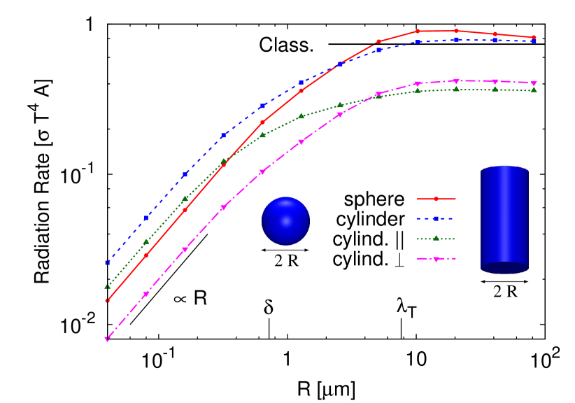
Figure 1: Heat radiation of a cylinder and a sphere of SiO₂, as function of $R$, normalized by the Stefan Boltzmann result, at $T=300K$. The horizontal line shows the radiation of a SiO₂ plate. $\lambda_{T}$ and the smallest skin depth $\delta$ in the relevant frequency range are marked on the $R$-axis. For the cylinder, the contributions of the different polarizations are shown.

Now we consider multiple objects. To compute $C^{neq}$ involving spheres or cylinders, we also need to convert among bases appropriate to the different objects. For example, for the experimentally most relevant configuration of a sphere and a plate Sheng et al. (2009), the radiation from the plate, given in a plane wave basis, must be transformed to the spherical basis et. al. (2009), reflected by the sphere, transformed back and so on. For simplicity, we focus on a plate held at a finite temperature $T_{p}\not=0$, while the sphere and environment are at zero temperature ( $T_{s}=T_{env}=0$). This suffices to describe also situations with $T_{s}\not=0$ as the transfer vanishes for $T_{p}=T_{s}$, and hence for $T_{s}\not=0$, we subtract our result evaluated at $T_{s}$. We express the correlations in Eq. (3) in a plane waves basis, and $H_{s}$, the energy absorbed by the sphere, is obtained by integrating $\mathbf{S}$ in Eq. (6) over two infinite parallel planes enclosing the sphere and separating it from the plate.

Figure 2 shows the results for the heat transfer from a SiO₂ plate at room temperature to a SiO₂ sphere of $R=5\mu$m at zero temperature, with surface-to-surface separation $d$, normalized by the Stefan-Boltzmann law $H_{s}=\sigma T^{4}2\pi R^{2}$ (only half of the sphere is exposed to the plate). For large $d$, $H_{s}$ is roughly 0.5 in these units, whereas for $d\to 0$, $H_{s}$ diverges due to the increased tunneling of evanescent waves, eventually exceeding the Stefan-Boltzmann value. The figure shows the numerical solution of Eq. (3) together with a one reflection approximation, where we set $\mathbb{O}_{\alpha,\beta}=(1-\mathbb{G}_{0}\mathbb{T}_{\beta})$ in Eq. (5), neglecting higher order reflections between sphere and plate. We see that the two curves approach each other for large $d$, as most rays are scattered outward and will not hit the sphere a second time. The reflection expansion is hence helpful for getting analytical results for $d\gg R$. Our numerical solution involves an expansion in spherical multipoles: For $R/\lambda_{T}$ large or $d/R$ small, increasingly more multipoles are needed. In practice, we restrict to a maximal multipole order of $l_{max}=20$, for accurate results up to $d\geq R/2$. Since closer separations are also interesting and relevant experimentally, but difficult numerically, we demonstrate in the inset of Fig. 2 the approach to a proximity transfer approximation (PTA), equivalent to the proximity force approximation (PFA) used in Casimir physics,

$$\lim_{d/R\to 0}H_{s}(d)=2\pi R\int_{d}^{d+R}S^{pp}(s)\,ds\,,$$ (8)

where $S^{pp}(d)$ is the Poynting vector for parallel plates at separation $d$. We identify the divergent terms as $d\to 0$ for both the sphere-plate and plate-plate configurations (the $E$ modes originating from evanescent waves), and evaluate their ratio in the one reflection approximation (allowing us to use $l_{max}=200$). As demonstrated in Fig. 2, this ratio approaches unity for $d\to 0$, suggesting $\mathbb{T}$ of the sphere approaches $\mathbb{T}$ of the plate in the PTA-sense. From this, we anticipate that multiple applications of these matrices (leading to the full solution) will also approach the ratio unity (independent of the accuracy of the one reflection approximation as $d\to 0$). We investigated different $R$ and confirmed that PTA in Eq. (8) is valid in general, with $H_{s}(d)\propto d^{-1}$ as $d\to 0$. While a similar point is discussed in Ref. Narayanaswamy and Chen (2008) for the case of two spheres and used in experimental studies Sheng et al. (2009); et. al. (2009), to our knowledge the validity of PTA was not quantitatively demonstrated previously. It is not obvious as it implies that the ratios $R/\lambda_{T}$ and $R/\delta$ are irrelevant as $d\to 0$.

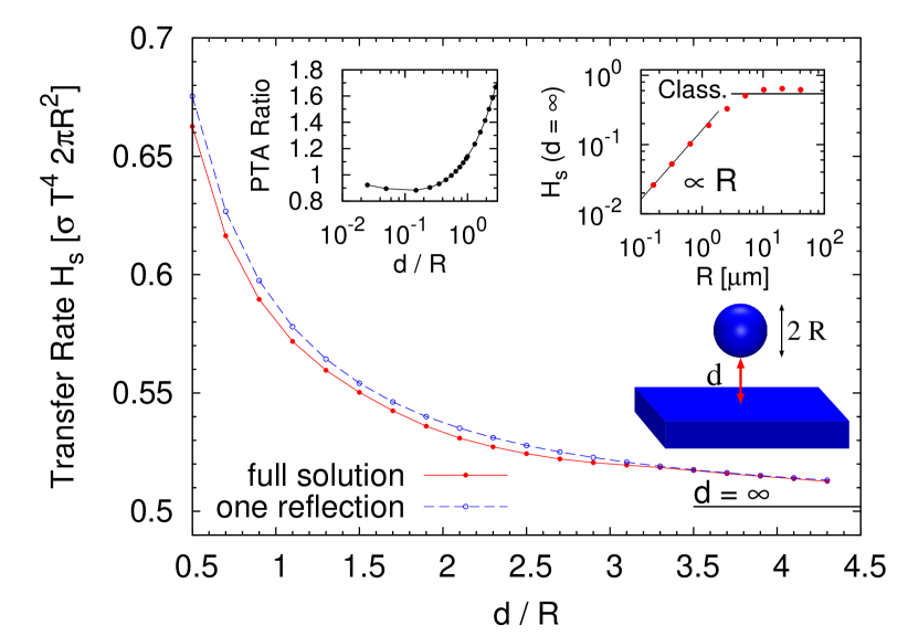
Figure 2: Heat transfer rate (in units of Stefan-Boltzmann’s law) from a room temperature plate to a sphere at $T=0$ of radius $R=5\mu$m (both SiO₂), as a function of separation. The horizontal bar shows the limit of $d\to\infty$. The left inset shows the approach to PTA for the divergent terms in a one reflection approximation. The right inset shows the result at large separation as function of $R$.

For $d\to\infty$, $H_{s}$ approaches a constant, which can be obtained by considering the $d$ independent part of the plate radiation, and using the one reflection term. The result, as shown in the right inset of Fig. 2, is quite similar to the behavior of a single sphere in Fig. 1: For small $R$, $H_{s}$ is proportional to the volume of the sphere, for similar reasons as discussed before. In this limit, $H_{s}$ is given by (with magnetic permeability of the sphere $\mu_{s}$ and Fresnel reflection coefficients $r^{E}$ and $r^{M}$ of the plate for angle $\theta$),

$$\lim_{d\gg\lambda_{T}\gg R}H_{s} =\frac{cR^{3}}{16\pi^{3}}\int_{0}^{\infty}\!d\omega a_{T}(\omega)\operatorname{Im}\left(\frac{\mu_{s}-1}{\mu_{s}+2}+\frac{\varepsilon_{s}-1}{\varepsilon_{s}+2}\right)$$

$$\int_{0}^{\pi/2}d\theta\sin\theta\sum_{P=E,M}(1-|r^{P}(\theta,\omega)|^{2}).$$ (9)

For $R\gg\lambda_{T}$, we may expect the result to approach a classical limit, given by $\sigma T^{4}e^{2}2\pi R^{2}$, with $e$ from Fig. 1. While the data points come close to this value, one does not expect exact approach Modest (2003), in contrast to Fig. 1, because the Fresnel coefficients depend on the angle of incidence. If we additionally let $(\varepsilon_{p},\varepsilon_{s})\to 1$, $H_{s}$ will approach the classical limit since the Stefan-Boltzmann law applies to all convex black bodies.

While we highlighted applications to simple shapes, the formalism presented here is more general, and combined with a numerical scheme for the computation of scattering matrices Rei can deal with collections of objects at different temperatures. Indeed, such a formalism is needed to properly deal with near field effects in device and fabrication at the micron scale. The formalism yields also Casimir forces between objects at different temperatures- examples of which we leave for future work. We note, however, that in the final stages of this project we became aware of two independent, partly related, studies of non-equilibrium effects Messina and Antezza ; Otey and Fan .