Distribution and excitation of thermal methanol in 6.7 GHz maser bearing star-forming regions

Abstract

Context. Candidate high mass star forming regions can be identified through the occurrence of 6.7 GHz methanol masers. In these sources the methanol abundance of the gas must be enhanced, as the masers require a considerable methanol path length. The place and time of origin of this enhancement is not well known. Similarly, it is debated in which of the physical components of the high mass star forming region the masers are located.

Aims. The aim of this study is to investigate the distribution and excitation of the methanol gas around Cep A and to describe the physical conditions of the region. In addition the large scale abundance distribution is determined in order to understand the morphology and kinematics of star forming regions in which methanol masers occur.

Methods. The spatial distribution of the methanol is studied by mapping line emission, as well as the column density and excitation temperature, which are estimated using rotation diagrams. For a limited number of positions the parameters are checked with non-LTE models. Furthermore, the distribution of the methanol abundance is derived in comparison with archival dust continuum maps.

Results. Methanol is detected over a $0.3\times 0.15$ pc area centred on the Cep A HW2 source, showing an outflow signature. Most of the gas can be characterized by a moderately warm rotation temperature (30$-$60 K). At the central position two velocity components are detected with different excitation characteristics, the first related to the large-scale outflow. The second component, uniquely detected at the central location, is probably associated with the maser emission on much smaller scales of 2″. Detailed analysis reveals that the highest densities and temperatures occur for these inner components. In the inner region the dust and gas are shown to have different physical parameters.

Conclusions. Abundances of methanol in the range $10^{-9}$ – $10^{-7}$ are inferred, with the abundance peaking at the maser position. The geometry of the large-scale methanol is in accordance with previous determinations of the Cep A geometry, in particular those from methanol masers. The dynamical and chemical time-scales are consistent with the methanol originating from a single driving source associated with the HW2 object and the masers in its equatorial region.

Figure 1: Sample spectra from the 3 positions identified in Sec. 3.2. Top spectrum at the ”Centre” position, coincident with the HW2 object. Bottom Left at the position of ”NE Outflow” and Bottom Right ”Envelope”. The small symbols at the top indicate the frequencies of methanol transitions in this band.

1 Introduction

While massive stars ($\gtrsim$10$M_{\odot}$) have an enormous impact on the evolution of the Galaxy, during their life and death, their birth process is still shrouded in mystery (e.g. Kurtz, 2005). To a large extent this is due to the environment in which the high-mass stars form. Most high mass stars are observed at large distances (compared to low mass stars), evolve rapidly, and form deeply embedded in their molecular clouds. Additionally, they typically form in clusters. Thus, very high resolution data are needed to resolve them and the disruptive influence they have on their direct environments (e.g. Martín-Pintado et al., 2005).

Methanol maser sources are exciting targets for the detailed study of high-mass star-formation. Continuum emission of warm dust at sub-millimetre wavelengths has been detected at well over 95% of the observed 6.7 GHz methanol maser sites (Hill et al., 2005), while 25% of the same masers are associated with a detectable ultra-compact (UC) HII region (Walsh et al., 1998). This seems to indicate that the masers probe a range of early phases of massive star formation and that the methanol maser emission disappears when the UC HII region is created (Walsh et al., 1998). The maser sources require high methanol abundance for their excitation, pointing to a recent release of methanol into the gas phase (van der Tak et al., 2000). We can thus expect to observe the thermal methanol lines in these sources, yielding diagnostics for the large scale kinematics and excitation. Besides being signposts, masers are excellent tracers of the geometry and small scale dynamics of these regions. Much effort has focused on studying the kinematics and several claims of circumstellar disks, expanding spherical shells and jets have been presented (e.g. Pestalozzi et al., 2004; Minier et al., 2002; Bartkiewicz et al., 2005, 2009). The evidence suggests that masers trace an evolutionary sequence or possibly a mass range in the formation process, or even both (e.g. Breen et al., 2010). However, it is not clear exactly with which of the physical structure(s) of the complex surroundings of young massive stars they are associated. By trying to make a link between the maser distribution and the large scale methanol kinematics and excitation, one can attempt to reach a better understanding of the physical and chemical state of the gas of the regions in which masers occur.

In order to carry out such a study, we have observed thermal methanol gas towards a sample of 15 high-mass star-forming regions for which we have very long baseline interferometry (VLBI) data of the 6.7 GHz methanol maser. The observations yield maps of the distribution and physical condition of the methanol gas in relation to the methanol maser. For one, the observations of the methanol allow one to probe a reasonably large range of temperature and density, due to its closely spaced $\Delta K=0$ ($\Delta J=1$) transitions with a large range in excitation energies and critical densities (Leurini et al., 2004). Moreover we can measure the methanol abundance and velocity field. Clearly, the methanol abundance needs to be significant in these regions ($>10^{-7}$, Sobolev et al., 1997); evaporation of $\mbox{CH}_{3}\mbox{OH}$ from the dust grains in these regions, at temperatures $\sim$100 K is thought to be responsible for this. This specific enhancement is supposed to be so short lived that it can be used as a chemical clock of the region (van der Tak et al., 2000). The enhancement can be used to determine the age of these regions and thus the evolutionary stage of the star formation process.

In this paper, we describe the observations and the procedure we have used to analyse the data. Because of its proximity and because a wealth of data exists on this source, we will focus on Cepheus~A East as a first example. The other sources will be presented in a second paper.

At a distance of 700 pc (Moscadelli et al., 2009), Cepheus A East is one of the closest high-mass star forming regions. The region has a luminosity of $2.3\times 10^{4}$  $\rm L_{\odot}$ (Evans et al., 1981) (scaled to the distance of 700 pc), out of which half is thought to come from the well-studied object HW2 (Garay et al., 1996), which is also the site of the 6.7 GHz methanol maser emission. The object shows both large scale molecular outflows over $\sim$1′ (Gómez et al., 1999) and signs of collapse over a similar extent (Bottinelli & Williams, 2004; Sun & Gao, 2009). At the core of HW2, a thermal jet extends over $\sim$2″ and proper motion outflow velocities of $\sim$500 km s^-1 have been measured in the radio (Hughes & Wouterloot, 1984; Curiel et al., 2006). Although a superposition of gas components at different positions cannot be completely ruled out (Brogan et al., 2007; Comito et al., 2007), the evidence is building that there is a disk at the centre of the jet, observable in both molecular gas and dust (Patel et al., 2005; Torrelles et al., 2007; Jiménez-Serra et al., 2007), as argued in detail in Jiménez-Serra et al. (2009). VLBI observations of the 6.7 GHz methanol maser suggest that the methanol masers arise in a ring-like structure, extending over $\sim$2″, straddling the waist of HW2 (Sugiyama et al., 2008; Vlemmings et al., 2010; Torstensson et al., 2011).

Table 1: $\mbox{CH}_{3}\mbox{OH}$ line data for the observed transitions, adopted from the CDMS (Cologne Database of Molecular Spectroscopy, Müller et al. (2005)). All lines are from the $J=7\to 6$ band, and throughout the paper a notation like “$-6$ E” refers to the $J=7_{-6}\to 6_{-6}$ E transition. Blended lines are indicated by a ^∗.

Frequency	$\mu_{g}^{2}S_{g}$	$E_{u}$	Transition
MHz	D2	K	$k$ type
337969.414	5.55	390.1	$-$1 A $\nu_{t}$=1
338124.502	5.65	78.1	0 E
338344.628	5.55	70.6	$-$1 E
338404.580	1.49	243.8	+6 E
338408.681	5.66	65.0	0 A
338430.933	1.50	253.9	$-$6 E
338442.344∗	1.49	258.7	+6 A
338442.344∗	1.49	258.7	$-$6 A
338456.499	2.76	189.0	$-$5 E
338475.290	2.76	201.1	+5 E
338486.337∗	2.77	202.9	+5 A
338486.337∗	2.77	202.9	$-$5 A
338504.099	3.80	152.9	$-$4 E
338512.627∗	3.81	145.3	$-$4 A
338512.639∗	3.81	145.3	+4 A
338512.856∗	5.23	102.7	$-$2 A
338530.249	3.82	161.0	+4 E
338540.795∗	4.60	114.8	+3 A
338543.204∗	4.60	114.8	$-$3 A
338559.928	4.64	127.7	$-$3 E
338583.195	4.62	112.7	+3 E
338614.999	5.68	86.1	+1 E
338639.939	5.23	102.7	+2 A
338721.630	5.14	87.3	+2 E
338722.940	5.20	90.9	$-$2 E

In Sec. 2 we describe the observations and calibration methods. The results are presented in Sec. 3 in the form of a number of sample spectra and maps of integrated line strength and velocity. In order to study the large scale methanol excitation we construct rotation diagrams and produce maps of the derived physical quantities in Sec. 4. We present non-LTE calculations for a number of positions to evaluate the limitations of the diagram analysis in Sec. 4.4. Subsequently we discuss estimates of the hydrogen column density before we present the methanol abundance in Sec. 4.6. The relation of our findings to the Cep A star forming process and in particular the occurrence of the methanol maser are discussed in Sec. 5.

2 Observations and data reduction

The JCMT observations of Cep A East (HW2) (22^h56^m17.9^s +62°01′49″ (J2000)) were performed on June 2 and June 17, 2007. We used the array receiver HARP, which has 16 receptors with a spacing of $\sim$30″ in a 4$\times$4 grid, resulting in a footprint of $\sim$2′. The receptors are single side-band receivers with a sideband rejection of $>$10 dB. We used the observing mode HARP5, a type of beam-switching (jiggle-chop) mode where several short scans at different positions of the target source (10 s per jiggle position) are observed before switching to the off position. As a result, several on-source observations share the same off-source observation which minimises the overhead while still providing good baselines. The observing mode results in a map of $20\times 20$ pixels covering 2′$\times$2′, thus each pixel is 6″x6″. This ensures proper Nyquist sampling of the 14″ telescope beam at 338 GHz.

The ACSIS correlator backend was set up with a 1 GHz (880 km s^-1) bandwidth and 2048 channels centred on the methanol $7_{0}\to 6_{0}$ A⁺ line at 338.41 GHz. The frequency set up allows us to cover 25 $\mbox{CH}_{3}\mbox{OH}$ lines (Table 1) with a velocity resolution of $\sim$0.43 km s^-1 (488 kHz). In total we have an effective (on source) integration time of $\sim$5 min per pixel with a typical system temperature ($T_{\mathrm{sys}}$) of $\sim$280 K. For our analysis we have adopted a main beam efficiency ($\mathrm{\eta}_{\mathrm{mb}}$) of 0.6. Regular pointings were done of the normal calibrators and we estimate to have an absolute pointing accuracy of $\approx$1″.

We used the Starlink package (Gaia and Splat) for initial inspection of the data. It was found that receptor R06 suffered from bad baselines (large ripples is some scans). For that receptor only these poor scans were removed, after which the scans were combined. The data were then converted to GILDAS/CLASS format and the remaining data reduction and analysis was performed in CLASS. A linear baseline was fitted to several spectral regions without any line emission and subtracted from the spectra. Next, to improve the signal to noise, the data were smoothed in the spectral domain resulting in a velocity resolution of 0.87 km s^-1 and an rms of $\sim 65$ mK.

The analysis was performed on a pixel by pixel basis, by first fitting a Gaussian to the strongest unblended line ($7_{-1}\to 6_{-1}$ E) in the spectra. The measured velocity and width of this line was then used to place windows around all other features in the spectra, for which the emission was integrated. Due to some overlap between different lines, only lines with a $>5\sigma$ ($\sim 0.6$ K km s^-1) detection are included in the subsequent analysis. In the centre area, at the position of HW2, a second velocity component can be distinguished. Where the two velocity components could be separated, manual analysis by fitting individual Gaussians to the lines was performed.

3 Results

3.1 Methanol lines

In the following we refer to each pixel in the map with its respective offset coordinates ($\Delta\alpha$, $\Delta\delta$), measured in arc seconds, with respect to the centre of the map (J2000 22^h56^m17.88^s +62°01′49.2″). Fig. 1 shows the observed spectrum at 3 positions: (+3″,3″) “Centre”, (+27″,+9″) “NE outflow”, (+21″,-3″) “Envelope”, where the designations can be understood from the forthcoming discussion in Sec. 3.2. Focusing at the centre spectrum, all but four of the detected lines are due to methanol (indicated by ticks at the top); the others are identified as SO₂, ³⁴SO₂ and H₂CS. The $\mbox{CH}_{3}\mbox{OH}$ K=+1 E line is a blend with another SO₂ line, also indicated in the figure.

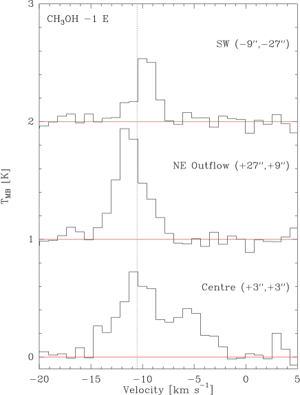
Figure 2: Velocity profiles of the -1 E line at 3 positions. Although the profiles are Gaussian in the outflow, there is a clear shift in the velocity. At the “Centre” position there are clearly two velocity components present. The dotted line is taken to be the system velocity, corresponding to the velocity of the dominant component at the “Centre” position.

In the centre spectrum, two gas components are observed: the main component with $v_{\rm lsr}=-10.5$ km s^-1 and a secondary red shifted at $-5.2$ km s^-1, as can be seen in the profile of the $-$1 E transition (Fig. 2). We note that the red-shifted velocity profile is overlapping with the range spanned by the methanol masers, which are observed with velocities between $v_{\rm lsr}=-4.6$ and $-1.5$km s^-1 (Torstensson et al., 2011). The red-shifted component is most readily identified in the higher-K transitions. While the first component is brightest in the low-K transitions and not detected in the higher-K lines, the $-5.2$ km s^-1 component is brighter in the higher-K lines and less bright in the lower-K lines. For the K=3 transitions, the two components are of similar strength. There is a weak detection of the methanol isotopologue ¹³$\mbox{CH}_{3}\mbox{OH}$ $J=13\to 12,\Delta k=+1$ in this component, indicating optical depth effects may be important for this. Also careful analysis, including averaging over a few pixels, shows that the torsionally excited $-1$ A v_t=1 line at 337.969 GHz is detected in the “Centre” region in the $-5.2$ km s^-1 velocity component.

Otherwise the observed line profile appears Gaussian in all components and does not show evidence of blue/redshifted wings. However, a modest velocity shift of the line is observed across the source with lower velocities to the NE and higher velocities to the SW (Fig. 2).

In order to start a consistent analysis of all methanol line emission in our data cube, we have extracted the integrated line flux from each line as described above (Sec. 2). To illustrate our procedure, we list the integrated line emission of the spectral features for the main velocity component at the “Centre” position from Fig. 1 in Table 2. For lines that are blended we have chosen a simple strategy. If the strengths ($S_{g}\mu_{g}^{2}$) of the lines are similar and they have comparable upper energy levels, we have split the measured flux between the two lines. If however one line has a significantly higher line strength and lower upper energy level we attribute all the emission to the strong line. In the case of the blend between the K=$-$2 A and K=$\pm$4 A, where the lines have comparable line strengths and energy levels we assume the total measured flux as an upper limit to all the lines.

Table 2: Line parameters for the main velocity component measured at the position of HW2 (+3″,+3″)

Line	Flux	Width
K, type	K km s-1	km s-1
0 E	2.16	4.21
$-$1 E	3.30	4.79
0 A	3.60	4.79
$-$6 E	0.03	1.74
+6 A	0.29	3.80
$-$6 A	0.29	3.80
$-$5 E	0.61	4.81
+5 E	0.31	3.15
+5 A	0.36	4.18
$-$5 A	0.36	4.18
$-$4 E	1.05	4.79
$-$2 A	2.00	4.79
+4 E	1.12	4.79
+3 A	1.37	4.79
$-$3 A	1.37	4.79
$-$3 E	0.93	4.07
+3 E	0.94	4.97
+2 A	1.42	5.38
+2 E	1.55	4.38
$-$2 E	1.55	4.38

3.2 Spatial distribution of methanol

Fig. 3 shows the spatial distribution of the flux, the central velocity, and the width of the methanol $7_{-1}\to 6_{-1}$ E line, which is the brightest unblended feature in the spectra. The methanol maser emission arises just to the NE of the centre of the map (+0.7″, +0.4″) and is indicated with a cross in all the figures. The white area in the maps represents regions where the line flux is less than our $5\sigma$ detection limit of 0.6 K km s^-1.

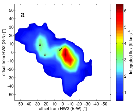
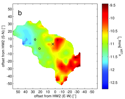
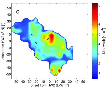
Figure 3: From top to bottom (a-c) the integrated flux, the velocity field, and the line width, of the methanol $7_{-1}\to 6_{-1}$ E-type transition, the strongest unblended line in the observed spectra. In all maps the cross marks the “Centre” position, the diamond “NE Outflow” and the circle indicates the position where the “Envelope” spectra are evaluated.

The line emission is constrained to an area, measured from the points furthest separated in the intensity map (Fig. 3a), with an extent of $\sim$85″ by 43″ ($\sim$0.29 pc by $\sim$0.15 pc), and is oriented in the NE-SW direction. The velocity map (Fig. 3b) shows that the methanol gas is entrained in an outflow with the blue-shifted emission to the NE and the red-shifted emission to the SW. Measured between the highest and lowest velocities in the map, the outflow has a modest velocity gradient of $\sim$3.1 km s^-1 over $\sim$0.20 pc. The integrated line flux peaks in the centre of the map at $\sim 5.2$ K km s^-1, with a bright extension to the SW over $\sim$13″($\sim$0.044 pc), which is associated with the red-shifted emission. Both the velocity field and line width maps (Figs. 3b and c) show a maximum in the centre of the map to the N of HW2. This is due to blending of the two velocity components that we are unable to decompose. A second maximum in the integrated line flux is observed $\sim$28″($\sim$0.095 pc) to the NE of the centre, which is associated with the blue shifted part of the emission and a secondary peak in the line width map. Throughout the paper we will refer to this position as the “NE outflow”. The quiescent methanol emission that is not associated with the outflows and does not show any peak in the integrated line flux map we will refer to as the “Envelope”.

4 Analysis

4.1 Rotation diagrams

From the above spectral cuts in 3 positions and the brightness distribution of one of the lines, it is clear that the observations trace a complex region in which the dynamic and excitation characteristics change, at least on the scales represented by the beam size of the telescope. To make a representation of the large scale distribution and excitation of methanol, we have created rotation diagrams (Boltzmann plots) at every pixel in order to be able to study the characteristics of the excitation distribution. Inherent to the method are a number of assumptions, namely that the gas at each velocity and spatial resolution element can be described by a single excitation temperature ($T_{\mathrm{rot}}\equiv T_{\mathrm{ex}}$), that all the lines are optically thin, i.e. $\tau<<1$, and that the size of the emitting region is the same for all lines. Although not all these assumptions may hold for all positions, the strength of the method is that it shows general trends on the relevant scales of our observations. In Sec. 4.4 we will test the validity of these assumptions.

For each pixel at which we measure at least three methanol transitions with S/N$>$5, we plot the upper energy level $E_{u}$ [K] of the transitions on the x-axis versus the logarithm of the column density in the upper energy state divided by the statistical weight of that upper level $\log(N_{\mathrm{u}}/g_{\mathrm{u}})$ on the y-axis. The weighted column density ($N_{u}/g_{u}$) can be calculated with Eq. 4.1 (Helmich et al., 1994) and the appropriate coefficients in Table 1. In the equation $Q(T_{\mathrm{rot}})$ is the partition function, $\mu$ the permanent dipole moment [Debye], $S_{g}$ the line strength value from (Blake et al., 1987), and $T_{\mathrm{MB}}$ the main beam temperature is the antenna temperature scaled by the main beam efficiency.

$$\frac{N_{u}}{g_{u}} = \frac{N_{\mathrm{M}}}{Q(T_{\mathrm{rot}})}e^{-E_{u}/T_{rot}}\approx\frac{1.67\cdot 10^{14}}{\nu\mu_{g}^{2}S_{g}}\int T_{\mathrm{MB}}dv$$ (1)

By fitting a straight line through these data points we determine the rotation temperature $T_{\mathrm{rot}}$ [K] and column density $N_{\mathrm{M}}$ [cm^-2] of the methanol gas. The rotation temperature is the negative inverse of the slope of the fitted line and the total column density is where the extrapolated line crosses the y-axis.

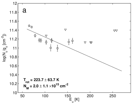
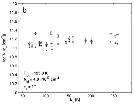
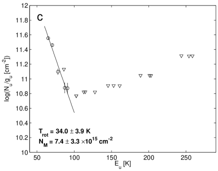
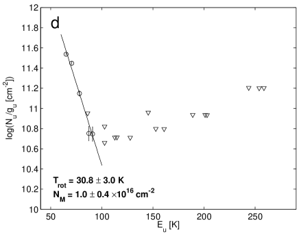
Figure 4: Rotation diagrams for three specific components and a population diagram for the fourth component identified in Sec. 3.2. Triangles indicate upper limits and error bars the 1$\sigma$ standard deviation in the flux determination. The diagrams displayed are: a: rotation diagram for the main, $-10.5$ km s^-1 velocity component at the ”Centre” position (+3″,+3″). b: population diagram for the red-shifted, $-5.2$ km s^-1 velocity component at the ”Centre” position (+3″,+3″); for this model asterisks indicate a best fit that includes optical depth effects and beam dilution (see Sec. 4.2), c: rotation diagram for the “NE Outflow” (+27″,+9″), d: rotation diagram for “Envelope” (+21″,-3″).

Fig. 4 shows the resulting rotation diagrams of the “Envelope” (the lower temperature quiescent gas), the “NE outflow”, and of the first velocity component at the “Centre” position of HW2. For the two positions in the outflow and envelope a single gas component provides a good fit to the data points with a rotation temperature of 30 K to 35 K and a column density of $10^{16}$ cm^-2. However, in the centre region things are more complex. The velocity component at $-10.5$ km s^-1 can be fitted by a straight line, yielding a rotation temperature of 224 K and a column density of 2$\times 10^{15}$cm^-2. For the $-5.2$ km s^-1 velocity component, the points lie nearly horizontal in the diagram and we would only able to put a lower limit of $>$300 K on the rotation temperature with the simple fit.

4.2 Population diagram modeling

Clearly the basic assumptions going into the rotation diagram analysis are violated for the “Centre” position and a successful explanation must accommodate both an apparent negative rotation temperature and the relative weakness of the low K lines for the red-shifted component. Non-LTE conditions, optical depth and beam-dilution effects can all play a role here. As a first step, to investigate the effect of line optical depth on the above results, we have adopted the method of Goldsmith & Langer (1999) which includes the source size ($\theta_{s}$) as a free parameter and allows for optical depth effects. We have performed a $\chi^{2}$ analysis for $10<T_{\rm rot}<500$ K, $10^{14}<N_{M}<10^{18}$ cm^-2, and $1\arcsec\ \leq\theta_{s}\leq 14\arcsec$, i.e. a beam dilution factor between 200 and 1. For the red-shifted component, we find the best fit to be for a rotation temperature of 125 K, a column density of $4\times 10^{17}$ cm^-2, and $\theta_{s}=1\arcsec$, much smaller than the beam. The merit of this model can be seen in panel Fig. 4b. In this specific case the maximum optical depth encountered was $\tau=6.8$. As this seems to be the component with the highest column density it is not surprising that ¹³$\mbox{CH}_{3}\mbox{OH}$ is detected in this component. Obviously, the highly excited K lines lead the model towards a high column density, but at the same time, the only way for the model to accommodate the lower K lines by increasing the optical depth is to decrease the source size. It should however be noted that this analysis assumes a single excitation temperature. We will discuss non-LTE modeling in Sec. 4.4.

4.3 Spatial distribution of the excitation

Maps of the derived rotation temperatures and column densities are presented in Figs. 6 and 6. In the maps we have excluded the results of the $-5.2$ km s^-1velocity component seen at the position of HW2. The methanol rotation temperature ranges from $\sim$20 K to $\sim$100 K over most of the map, but shows a pronounced peak of $\gtrsim$200 K close to the HW2 position. We find column densities between $10^{15}$ cm^-2 and $3\times 10^{16}$ cm^-2. Overall, the methanol column density distribution is quite smooth, showing a minimum towards the centre position. In Sec. 4.4 we will investigate whether this minimum is an artifact of the rotation diagram method. Additionally, some care must be taken when analysing the results in the centre region. Only at the position of HW2 are we able to separate the two velocity components of the gas. In the neighbouring pixels the integrated line fluxes are therefore overestimated due to blending.

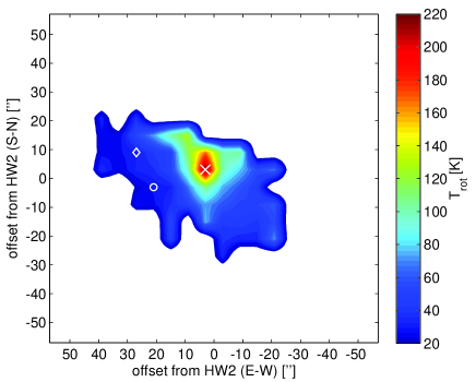
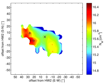
Figure 5: Map of derived rotation temperatures. Symbols are as in Fig 3.

Figure 6: Map of derived column densities. Symbols are as in Fig 3.

4.4 Non-LTE analysis

4.4.1 Method

In order to check the validity of the assumptions of the rotation diagram analysis, we have run a set of non-LTE models. By comparing the resulting synthetic spectra with the observed spectra, these models also allow us to investigate the physical conditions (i.e. temperature and density) at distinct positions in the methanol emitting region. We have used the RADEX package, that uses statistical equilibrium for the population calculations and an escape probability method to calculate the optical depth (van der Tak et al., 2007). The main assumptions are that the medium is uniform and that the optical depth is not too high ($\lesssim 100$). The most accurate collisional rates are available for the first 100 levels of methanol (Pottage et al., 2004; Schöier et al., 2005) and we therefore restrict this part of the analysis to the 24 relevant lines from Table 1.

Initial runs of the non-LTE model indicated that the methanol excitation is more strongly governed by the density than the temperature. Using a uniform sphere geometry, we considered kinetic temperatures between 30 and 300 K and $\mbox{H}_{2}$ densities between $10^{4}$ and $10^{7}$ cm^-3. Even at the lowest temperature all the lines, except the K=$\pm$5 and K=$\pm$6, are excited in the high-density case. On the other hand, at low-density and high-temperature, only the lowest three K levels (K=0,$\pm$1,$+$2) are populated. A combination of high temperature and high density is required to excite all lines, making this methanol band useful as a density and temperature tracer (Leurini et al., 2004).

Starting with model values comparable to the results from Sec. 4.1, it is possible to model the observed line strengths of the large-scale emission with the simple assumption that the emitting region is filling the beam. For these parameters all the lines are optically thin ($\tau$ ¡ 0.3), validating the assumption made in the rotation diagram analysis for the large scale emission.

In the above calculations the background radiation field was represented by the cosmic microwave background with $T_{\mathrm{bg}}$=2.73 K. Models with background radiation temperatures in the range 3 – 300 K were run, but this has no clear impact on the lines considered here. Mostly the contrast of the lines with respect to the background was reduced without changing their relative intensities. This result can be understood from the fact that our models consider only the torsional-vibrational ground state of methanol (Leurini et al., 2007). These models are inconclusive about the influence of the radiation field, which are expected to be important in the maser region.

4.4.2 Non-LTE results

Next, we use the non-LTE calculations to fit the spectra for the four regions identified in Sec. 3.2 (both velocity components at “Centre”, the “NE outflow”, and the quiescent gas in the “Envelope”). In a search for minima of the reduced $\chi^{2}$ we have used a model grid that includes column densities from 10¹³ to 10¹⁹ cm^-2 at every half dec, densities from $10^{4}$ up to 10⁹ cm^-3, kinetic temperatures between $30-300$K, and radiation temperatures in the range $3-400$K. Based on our findings in Sec. 4.1 we have adopted a beam dilution factor of 50 for the red-shifted emission in the “Centre”, corresponding to the 2″ extent of the region where the masers appear. It is found that the models are able to reproduce the lines at all four positions to within 5-10% accuracy. In Fig. 7 we plot the observed integrated flux and the synthetic integrated flux calculated with RADEX versus 7${}_{\mathrm{K}}\to$6_K number. Also indicated is our 3$\sigma$ detection limit.

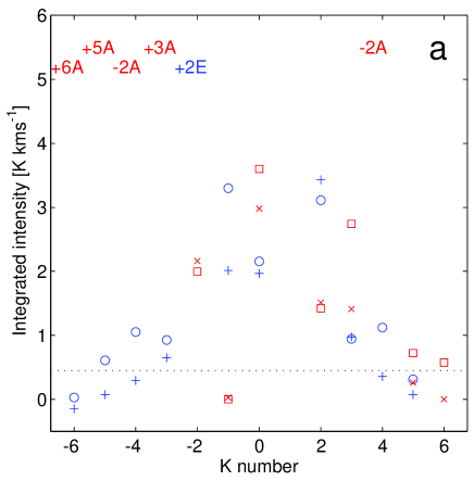
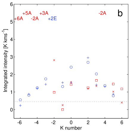
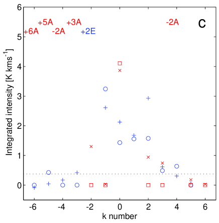
Figure 7: Plots of the integrated intensity for different $\mbox{CH}_{3}\mbox{OH}$ $7_{\mathrm{K}}\to 6_{\mathrm{K}}$ transitions and the best $\chi^{2}$ model values. In the panels the observed flux (open symbols) is plotted, as well as the non-LTE model values (plusses and crosses). Also indicated is the 3$\sigma$ detection limit. Circles and plusses (blue) are used for E-type lines and squares and crosses (red) for A-type. Labels on the top identify blended lines, for which the combined flux and model value are displayed. The K=+1 line which is blended with an SO₂ was not included in the analysis for the centre region components (top panels). The parameters of the fits are listed in Table 3. a: main, $-10.5$ km s^-1 velocity component at the “Centre” position with beam dilution factor of 1, b: red-shifted, $-5.2$ km s^-1 velocity component at “Centre” with a beam dilution factor of 50, c: the “NE Outflow” and d: “Envelope”.

Like before, this analysis is complicated somewhat by the blending of lines, both by methanol and in the case of the K=+1 E by blending with SO₂. In the case of the K=+1 E line we have not included it in the analysis of the centre position components as the SO₂ contributes significantly to it. For the “NE outflow” and for the “Envelope” the SO₂ does not appear to contribute significantly, as the other SO₂ line is not detected, and we have included it in the analysis. At the position of HW2 the methanol gas is highly excited and the blending of methanol lines becomes more severe and confusion prevents one from detecting the higher (K$\geq 5$) lines. Also, at this position the K=$\pm 2$ lines show a large ($\sim 50$%) deviation from the RADEX model. The reason for this discrepancy is yet unclear, but could be another indication that we are not complete in treating radiative processes.

Table 3: Results of the non-LTE models.

Position	$\Delta\alpha$a	$\Delta\delta$a	log(NM)	Tkin	log(n${}_{\mathrm{H_{2}}}$)	Trad
	″	″	cm-2	K	cm-3	K
Centre, main	+3	+3	${16.0}$	$90$	${4.0}$	30
Centre, red-shifted b	+3	+3	${17.0}$	$130$	${7.0}$	100
Outflow (NE)	+27	+9	${15.0}$	$90$	${5.0}$	30
Envelope	+21	-3	${15.0}$	$90$	${5.0}$	30

^a Offset from centre of map RA 22^h56^m17.88^s, DEC +62°01′49.2″.

^b This component was modeled with a beam dilution factor of 50.

The results of our non-LTE analysis are summarised in Table 3. The coolest and most diffuse gas is found in the envelope and outflow, where one should take into account that the granularity of the model grid probably prevents the distinction of small temperature and density differences. In comparison, the gas associated with the rotation temperature peak is much denser and also warm. We find the highest density and temperature in the “Centre” HW2 position where the maser emission occurs. However, given the large beam dilution and the limited set of available levels for collisional and radiative excitation, these numbers should be treated cautiously.

The non-LTE analysis confirms that there are no large column density gradients across the source. But although generally the values are in agreement with our rotation diagram analysis, they differ in details. In particular, the non-LTE analysis finds local maxima of column density in the “Centre” components. Although some shortcomings are demonstrated for the inner components, the rotation diagram maps are useful for outlining the qualitative large-scale properties and constraining the distribution of the excitation; running pixel based non-LTE models is beyond the scope of this paper.

4.5 $\mbox{H}_{2}$ column density

In order to estimate the methanol abundance we require a measure of the $\mbox{H}_{2}$ column density to combine with the estimates of the methanol column density. Therefore we used the SCUBA map of Bottinelli & Williams (2004) and derived the $\mbox{H}_{2}$ column distribution using the formula of Henning et al. (2000) (eq. 2), where $S_{\nu}$ is the flux in Jy beam^-1, $\kappa_{d}(\lambda)$ the dust opacity at the observed wavelength, $\Omega_{mb}$ the solid angle of the main beam, $B_{\nu}(T)$ the Planck function (Black body), $m_{H}$ the mass of the hydrogen atom, and $R$ is the gas to dust ratio. In the calculation we have used: $\kappa_{d}(875\mathrm{\mu m})=1.4$ and $R$=150 (Henning et al., 2000).

$$N(H_{2}) = \frac{S_{\nu}}{\kappa_{d}(\lambda)\Omega_{mb}B_{\nu}(T)2m_{H}}R$$ (2)

The calculations were run for two cases. In the first case, we assume a constant dust temperature of $T_{\mathrm{d}}$$=30$ K to derive the $\mbox{H}_{2}$ column density and the methanol abundance, $X_{\mathrm{M}}$. In the second case we have assumed the dust temperature $T_{\mathrm{d}}$ to be equal to the rotation temperature that we derived from the rotation diagram analysis in Sec. 4.1 and used that as input to the black body function.

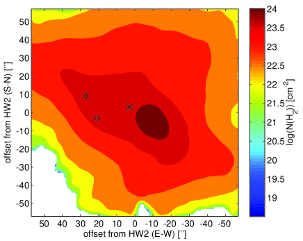
Figure 8: H₂ column densities derived from the SCUBA dust continuum for a constant dust temperature of 30 K.

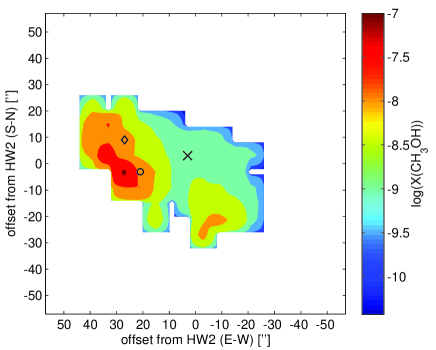
Figure 9: Methanol abundance derived from the methanol column densities obtained in the rotation diagram analysis and the H₂ column densities obtained for the constant dust temperature 30 K.

4.6 Methanol abundance

The results of the constant temperature hydrogen column density and methanol abundance calculations are presented in Figs. 8-9. The resulting hydrogen column density Fig. 8, is the SCUBA map (by Bottinelli & Williams (2004)) scaled by a constant factor to convert it from Jy beam^-1 to $N$(H₂) in cm^-2. The result is a very smooth map with $\mbox{H}_{2}$ column densities between $\sim 10^{21}$ cm^-2 and $\sim 10^{24}$ cm^-2. The general morphology of the dust emission is similar to that of the methanol gas, though notably the dust emission does not peak at the position of HW2 but further to the SE at position (-9″,-4″).

Similarly, the methanol abundance map derived with a constant dust temperature, Fig. 9, shows the same structure as the column density map, since there are no large variations in the SCUBA dust map. We derive a methanol abundance of $X_{\mathrm{M}}\sim$10^-8.5 for the central region. As noted before, the distribution is relatively flat, and probably not very accurate for the centre position.

In the second case, when we used the methanol rotation temperature as a measure of the dust temperature, we find the resulting $\mbox{H}_{2}$ column density to be anti-correlated to the rotation temperature, as the high rotation temperatures derived for the centre region then result in a lower $\mbox{H}_{2}$ column. In this way we would derive a $\mbox{H}_{2}$ column of $\sim 10^{22}$ cm^-2 (much lower than inferred earlier $\sim 10^{24}$ cm^-2; Martín-Pintado et al., 2005). Although we have already encountered the limited validity of the rotation diagram for the “Centre” region in Sec. 4.4.2, it is clear that there must be a mismatch between the gas and dust temperature on the scales of the JCMT maps. Both the rotation diagram and non-LTE calculations indicate higher temperatures towards the centre, for which there is little evidence in the dust images, which even peak at an offset of $\sim$10″ from the rotation temperature maximum. Besides the possibility that the rotation temperature is not a good estimate of the kinetic temperature of the gas, it seems plausible that the kinetic temperature of the gas is not equal to the dust temperature at these locations. Therefore, we adopt a constant dust temperature of 30 K to estimate the H₂ column density and $\mbox{CH}_{3}\mbox{OH}$ abundance, realizing that this method will overestimate $N$(H₂) at the centre of the map.

5 Discussion

5.1 Outflow morphology

We have presented maps of the large scale distribution of the thermal methanol associated with Cep A East (Figs. 3, 6 and 6). The emission is constrained to a region of size 0.29 $\times$ 0.15 pc (85″ $\times$ 43″), roughly centred on the location of the radio continuum source HW2, the most massive YSO in the region. Moreover, the velocity field shows that the methanol gas is entrained in a large scale bipolar outflow. The position angle of this outflow appears consistent with the HW2 geometry and earlier results (Gómez et al., 1999).

While the largest flux of the K=-1 E line Fig. 3a is associated with the receding part of the outflow (towards the SW), coincident with the SCUBA peak, the most energetic gas appears at the opposite side of HW2. This is evident already in the velocity width distribution of the brightest line, that has a line width of $>$4 km s^-1, to the NE of HW2, Fig. 3c. It becomes more clear when the temperatures are derived from rotation diagram analysis, the rotation temperature peaks to the NE of HW2 at $\sim$200 K (Fig. 6).

Several authors (Patel et al., 2005; Jiménez-Serra et al., 2007; Torrelles et al., 2007) have inferred obscuring gas in a flattened circumstellar structure of $\sim$1″ (700 AU) surrounding HW2. The gas shows signs of rotation and is perpendicular to the high velocity outflow ($\sim$500 km s^-1) seen in the radio continuum (Curiel et al., 2006). The molecular outflow that we observe in methanol is blue-shifted to the NE, which implies that this side of the outflow is pointing towards the observer, Fig. 3b. Torstensson et al. (2011) propose a model in which the methanol maser emission arises in a ring-structure in the equatorial plane of HW2. In contrast to the circumstellar molecular material, the masers do not show signs of rotation; rather the observations seem to indicate an infall signature. It is argued that the masers occur in the shock interface between the circumstellar disk and inflow regulated by a large scale magnetic field (Vlemmings et al., 2010). Torstensson et al. (2011) derive an inclination of 67.5°and a position angle of 9.3° for the ring. The masering gas occurs on size scales of $\sim$2″ and is very likely clumpy on smaller scales $\sim$0.1″(Minier et al., 2002). At the resolution of the observations presented in this paper the masering gas can clearly not be resolved, nevertheless the geometry that is observed on smaller scales suggest that to the NE of HW2 we have a line of sight into the outflow probing highly excited gas close to the protostar, which explains why we see such a high rotation temperature in this region. Evidence for such wide-angle molecular outflow has recently been presented by Torrelles et al. (2010).

5.2 Methanol distribution

The highest methanol temperatures appear to occur close to the HW2 central source, but we have demonstrated in Sec. 4.6 that the dust emission is not showing the same distribution. It seems plausible that the highest methanol rotation temperatures occur in a region where the dust is at least partly destroyed, possibly at the onset of the outflow where the evaporation from the grains occurs that produces the methanol gas in the first place. The considerations on the dust distribution force us to adopt a constant dust temperature in our abundance analysis. On small radii this may have two effects: firstly, the gas to dust ratio may be higher due to grain destruction, which increases $N$(H₂) and lowers the abundance. Secondly, the dust temperature may be higher than 30 K, which decreases $N$(H₂) and increases the abundance. Increasing the gas-to-dust ratio from 150 to 200/250 decreases the abundance with a factor of 0.75/0.60 respectively. Increasing the dust temperature to 60/100/300 K increases the resulting abundance by a factor of 2.3/4.1/13.0 respectively. High optical depth of the dust will lower the derived abundance. These arguments show that at the peak rotation temperature, the methanol abundance is quite sensitive to increased dust temperatures, but is probably correct to within an order of magnitude, without taking beam-dilution effects into account.

The derived abundances of $\sim 10^{-8.5}$ are higher than expected from gas-phase chemistry, but lower than seen in the solid state (Gibb et al., 2004). High optical depth of the lines is ruled out by the excitation calculations, except in the central region. However, it is possible that there the local methanol abundance is still higher. For example, the methanol maser occurs on much smaller scales than those we are probing in these JCMT observations. The total extent of the $\mbox{CH}_{3}\mbox{OH}$ maser is $\sim<$2″. Moreover, we found that the same small scale enhancement can explain the peculiar excitation of the “Centre” region. This strengthens the idea that the highly excited methanol gas emission is coming from the same region. Assuming that the dust and the corresponding $\mbox{H}_{2}$ is smoothly distributed, this component can have higher column density because of the optical depth and beam-dilution, resulting in methanol abundance estimate of $\sim 10^{-7}$ locally. This value is similar to previous values by other authors for maser regions (Menten et al., 1986, 1988) and still higher than expected from gas-phase chemistry and lower than seen in the solid state. Possibly the methanol evaporated from grain mantles some time ago ($\sim$1000 yr) and is now destroyed by chemical reactions and/or photo-dissociated.

As noted earlier, all the methanol gas seem to be entrained in an outflow, spanning 0.29 pc. The outflow is oriented close to the plane of the sky, assuming an inclination of 67.5° (Torstensson et al., 2011) we find an outflow velocity of $\sim$5.8 km s^-1. The result implies a dynamical timescale of $\sim 2.4\times 10^{4}$ yrs. The dynamical timescale agrees well with the chemical timescale (a few $10^{4}$ years) for which such a methanol enhancement is believed to be possible (van der Tak et al., 2000). This supports the argument of a common driving source for all the methanol gas in the region. Alternatively, the methanol may be released in the wake/outflow cavity of the jets described by Cunningham et al. (2009): the uv-radiation produced in the shock interface may shine back into the cavity and photo-desorb the methanol, causing a local enhancement in the methanol column density.

5.3 Physical conditions

The rotation diagram analysis shows rather warm gas entrained in a large scale outflow. Although the non-LTE analysis demonstrates that the methanol band used in this study is quite sensitive to collisional excitation, even in the low temperature regime, it confirms qualitatively the large scale presence of warm methanol gas. Over large areas of the source the total methanol column density appears to be fairly constant at $\sim 10^{15}$ cm^-2, assuming a uniform distribution with unity beam-filling factor.

The fidelity of the rotation diagrams is breaking down particularly in the centre area, where higher excitation lines appear. Especially the red-shifted component requires non-LTE excitation and/or beam-dilution effects to be explained. At these locations a complete analysis requires high resolution data and non-LTE modeling including excitation by infrared radiation. That more methanol levels should be taken into account is demonstrated by the detection of the torsionally excited $-1$ A v_t=1 line at 337.969 GHz in the red-shifted component (Leurini et al., 2007). Radiative pumping is also expected from models of methanol maser excitation (Cragg et al., 2005; Sobolev & Deguchi, 1994; Sobolev et al., 1997)

5.4 Origin of maser emission

Although a larger area around Cep A has been searched for maser emission (Torstensson et al., 2011), only one place in this source, so abundant in methanol, does show maser emission. We find the maser position to contain warmer gas than the other positions, probably the highest column density, and certainly the density appears to have a maximum here at $\sim 10^{7}$ cm^-3. Moreover, this position does stand out as the position where a second kinematic component at $-5.2$ km s^-1 is found. Special properties for this component are the detection of the torsionally excited line, and the requirement to invoke a large beam dilution to explain the ratios of the higher excited lines. This dilution factor matches quite well with the size of the area of $<2$″ over which masers are detected (Sugiyama et al., 2008; Torstensson et al., 2011). Combining these facts, we identify this component with the origin of the maser action. We note that the densities we derive for this component are still below $10^{9}$ cm^-3, where the maser lines would be quenched according to model calculations (Cragg et al., 2005). The models have methanol temperature ranges and methanol column densities that are consistent with our estimates, but it is hard to test the dust temperature, which must be $>$100 K for the maser excitation. We note that many of the values estimated here are inferred indirectly and the relevant processes may occur on even smaller scales than reflected by the beam-dilution factor.

The central abundance of $X_{\mathrm{M}}\sim 10^{-7}$ is not in excess to that found in low-mass star-forming regions, but the methanol column density $N_{\mathrm{M}}\sim 10^{17}$ cm^-2 clearly is (Maret et al., 2005). This could point to the condition that the high-density, high-temperature region in low-mass star-forming regions is too small to produce a path length long enough, with sufficient methanol column density, to produce maser emission. Jørgensen et al. (2002) show the high-density, high-temperature region for a low-mass protostar to be $\sim$10-30 AU. In contrast, for a high-mass protostar, the region extends over $\sim$1000 AU (Doty et al., 2002), possibly facilitating the necessary amplification. Alternatively, Pandian et al. (2008) suggest that in low-mass stars the critical infrared pumping is only available in the inner region, where the density is so high that the maser will be quenched. Both effects favour maser emission in the environments of high mass protostars and explain that the masers occur on rather large distances from the central object (Torstensson et al., 2011).

To further constrain the physical conditions at the position of the methanol maser and discern radiation and density effects, high-J and $\nu_{t}=1$ line observations are required, for example with the CHAMP+ instrument on the APEX telescope. To probe the excitation of methanol gas on small scales (comparable to that of the maser emitting region) high resolution interferometry observations are needed, with instruments such as the SMA and the IRAM interferometers, and in the longer term, for lower declination sources, ALMA. The interpretation of these observations requires models that include the excitation of CH₃OH by infrared radiation.