A linear framework for region-based image segmentation and inpainting involving curvature penalization

Abstract

We present the first method to handle curvature regularity in region-based image segmentation and inpainting that is independent of initialization.

To this end we start from a new formulation of length-based optimization schemes, based on surface continuation constraints, and discuss the connections to existing schemes. The formulation is based on a cell complex and considers basic regions and boundary elements. The corresponding optimization problem is cast as an integer linear program.

We then show how the method can be extended to include curvature regularity, again cast as an integer linear program. Here, we are considering pairs of boundary elements to reflect curvature. Moreover, a constraint set is derived to ensure that the boundary variables indeed reflect the boundary of the regions described by the region variables.

We show that by solving the linear programming relaxation one gets quite close to the global optimum, and that curvature regularity is indeed much better suited in the presence of long and thin objects compared to standard length regularity.

1 Introduction

Regularization is of central importance for many inverse problems in computer vision including image segmentation and inpainting Mumford-Shah-89 ; Chan-Vese-01 ; Masnou-Morel-98 ; Bertalmio-et-al-00 ; Tschumperle-06 ; Bornemann-Maerz-07 . The introduction of higher-order regularizers in respective energy minimization approaches is known to give rise to substantial computational challenges. Some of the most powerful approaches to image segmentation are based on region integrals with regularity terms defined on the region boundaries Blake-Zissermann-Book-87 ; Mumford-Shah-89 ; Nitzberg-Mumford-Shiota-93 ; Boykov-Jolly-01 ; Chan-Vese-01 ; Esedoglu-March-03 ; Klodt-et-al-08 . While many such methods make use of length as a regularity term, only few use curvature regularity. This is in contrast to psychophysical experiments on contour completion Kanizsa-71 where curvature was identified as a vital part of human perception. Note that curvature regularity is qualitatively different from length regularity. As shorter boundary curves are preferred in the length case, this causes the well-known shrinking bias. This is not the case for curvature, since the total curvature of any closed, convex curve is equal to $2\pi$.

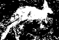
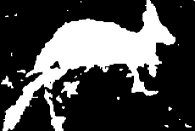
Input with seeds	thresholding scheme	with length regularity	with length and curvature

Figure 1: With the proposed method, long and thin structures are much better handled than with length-based approaches.

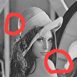
damaged image	with length regularity	with curvature regularity

Figure 2: Curvature regularity on the level lines improves inpainting.

Length regularization has become an established paradigm as there exist many powerful algorithms for computing optimal solutions for such energy functionals, either using discrete graph-theoretic approaches based on the min-cut/max-flow duality Greig-Porteous-Seheult-89 ; Boykov-Jolly-01 or using continuous PDE-based approaches using convex relaxation and thresholding theorems Nikolova-Esedoglu-Chan-06 . Region-based problems for segmentation using curvature regularity have typically been optimized using local optimization methods only (cf. Nitzberg-Mumford-Shiota-93 ; Esedoglu-March-03 ). As a consequence, experimental results highly depend on the choice of initialization. Moreover, these methods do not offer any insights concerning how close the computed solution is to the (unknown) global solution.

In this paper, we propose a relaxed version of region-based segmentation which can be solved optimally. The key idea is to cast the problem of region-segmentation with curvature regularity as an integer linear program (ILP). By solving its LP-relaxation and thresholding the solution we obtain a solution to the original integer problem and are able to evaluate a bound on its quality with respect to the globally optimal solution. In addition, we show that the method readily extends to the problem of inpainting.

Figure 1 demonstrates that the proposed method allows segmenting objects in a way which preserves perceptually important thin and elongated parts. The found solution is within $1.3\%$ of the global optimum. Figure 2 demonstrates the superior performance of curvature regularity over length regularity in a corresponding inpainting experiment.

Existing Work on Curvature Regularity.

For contour- or edge-based segmentation methods researchers have successfully developed algorithms to optimally impose curvature regularity using shortest path approaches Amini-et-al-90 or ratio cycle formulations Schoenemann-Cremers-07b on a graph representing the product space of image pixels and tangent angles Parent-Zucker-89 . In the region-based settings considered, curvature is usually handled by local evolution methods Chan-Kang-Shen-02 ; Esedoglu-March-03 ; Nitzberg-Mumford-Shiota-93 ; Tschumperle-06 . Among the methods that pre-date our conference publication Schoenemann-Kahl-Cremers-09 , the only exception we are aware of is the inpainting approach of Masnou and Morel Masnou-Morel-98 who can optimize the $L_{1}$-norm of the curvature in the absence of regional data terms using dynamic programming.

In this paper we propose an LP-relaxation approach to minimize curvature in region-based settings. In contrast to Masnou-Morel-98 it allows imposing arbitrary functions of curvature and arbitrary data terms. The algorithmic formulation is based on the concepts of cell complexes and surface continuation constraints which have been pioneered by Sullivan Sullivan-94 and Grady Grady-10 in the context of 3D-surface completion.

The present paper is based on our preliminary work in Schoenemann-Kahl-Cremers-09 , but contains several novelties. Firstly, we show that the constraint system in Schoenemann-Kahl-Cremers-09 needs to be augmented by additional constraints in order to ensure that the boundary of the region-based segmentation is correctly estimated. Secondly, we discuss the connections of our method, when restricted to length regularity, with standard methods for length regularity and compare experimentally. In addition, the original inpainting method has improved by incorporating a boundary estimation scheme.

There has been a subsequent paper by El-Zehiry and Grady ElZehiry-Grady-10 which optimizes the same model as in our original paper, but applies quadratic pseudo-Boolean optimization (QPBO) for obtaining the solution. In the case of a square grid, QPBO is able to efficiently compute a solution with curvature regularization, and with a subsequent probing stage often the global optimum is found. However, the discretization artefacts are severe for a cell complex of squares. Better connectivities can only be handled approximately.

The source code associated to this paper is freely available at http://www.maths.lth.se/matematiklth/personal/
tosch/download.html.

2 Length-based Segmentation Problems

To detail the proposed method for curvature regularity, we first introduce a novel method for length-based segmentation problems. In practice there are more efficient algorithms for this problem Boykov-Kolmogorov-03 ; Nikolova-Esedoglu-Chan-06 , but in contrast to them the presented one is easily extended to curvature. A comparison to the known techniques is given at the end of this section.

Given an image $I:\Omega\rightarrow I\!\!R$, the problem is to segment it into two regions, foreground and background. Here “region” means an arbitrary subset of $\Omega$, i.e. there can be several disconnected components and each one can have holes. Hence, each point $\mathbf{x}\in\Omega$ is to be assigned a region $u(\mathbf{x})\in\{0,1\}$ where $0$ denotes background, $1$ foreground.

The desired segmentation is defined as the global optimum of an energy function, consisting of two terms. The first one is called the data term and specified by a function $g_{0}(\mathbf{x})$ for points belonging to the background and a function $g_{1}(\mathbf{x})$ for the foreground. Both functions will generally depend on the input image $I$. In addition there is a regularity term that penalizes the length of the segmentation boundary by a weighting parameter $\nu\geq 0$. The arising energy minimization problem to be solved is

$$\min\limits_{u:\Omega\rightarrow\{0,1\}} \int\limits_{\Omega}g_{0}(\mathbf{x})[1-u(\mathbf{x})]\,d\mathbf{x}\,+\,\int\limits_{\Omega}g_{1}(\mathbf{x})\,u(\mathbf{x})\,d\mathbf{x}$$ (1)

$$\hskip 28.45274pt+\,\nu\,|C|\ \ \ ,$$

where $C=\partial\{\mathbf{x}\,|\,\nabla u(\mathbf{x})=\mathbf{0}\}$ is the set of points where $u$ is discontinuous (i.e. “jumps” from $0$ to $1$) and $|C|$ denotes its one-dimensional measure. In other words, $C$ is a set of closed lines (which may include parts of the boundary of $\Omega$) and $|C|$ denotes the sum of the length of all lines.

For convenience, we reformulate (1) by splitting the integrand of the first term into a constant term and one depending on $u$. Defining $g(\mathbf{x})=g_{1}(\mathbf{x})-g_{0}(\mathbf{x})$ the resulting functional is

$$\min\limits_{u:\Omega\rightarrow\{0,1\}} \int\limits_{\Omega}g(\mathbf{x})\,u(\mathbf{x})\,d\mathbf{x}\ +\nu\,|C|\ +\ \mbox{const}\ \ .$$ (2)

In the following we will ignore the constant except when evaluating relative gaps between a lower bound and the energy of some segmentation.

2.1 Discretization

In this paper we consider discretized segmentation problems where instead of optimizing infinitely many values $\{u(\mathbf{x})\,|\,\mathbf{x}\in\Omega\}$ we only consider finitely many “basic regions” and jointly assign all points in a basic region to the same segment. Note that in practice we will always get a discrete input image $I$, where the basic regions are given by pixels. Hence, the data term by itself will produce such an assignment even for the continuous problem. This is no longer true when the regularity term is added, but in practice the discretized energy function can be designed to account for this phenomenon Boykov-Kolmogorov-03 ; Nikolova-Esedoglu-Chan-06 .

We require that our set of basic regions – denoted $\mathcal{F}$ – be a cell complex and a partitioning of $\Omega$, i.e. that (1) no two regions overlap and (2) the union of all basic regions yields $\Omega$. An example is given in Figure 3 (a).

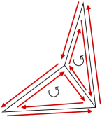
(a)	(b)

Figure 3: The basic concepts of our method. (a) A cell complex. (b) The method considers oriented regions and oriented boundary elements.

The presented approach makes use of another essential part of a cell complex: boundary segments. These are the line segments that form the borders of the basic regions. Usually a boundary segment has two neighboring regions, except for segments at the border of $\Omega$ where there is only one. The set of all boundary segments is denoted $\mathcal{E}$. As will be shown below we need to consider both possible ways of traversing a boundary segment. Hence, for each boundary segment we consider two oriented boundary segments, also called line segments in the following. The set of all these segments is denoted $\mathcal{E}^{O}$ and $\ell(e)$ will denote the length of a line segment $e$.

In essence, the data term will be defined in terms of the basic regions, the regularity term in terms of boundary segments. To approximate the continuous problem sufficiently well, basic regions should generally not correspond to pixels. Instead, as detailed in Figure 4 we split the pixels into either $4$ or $32$ basic regions, induced by lines with $8$ and $16$ different directions respectively. In the following we will refer to this as $8$- and $16$-connectivity.

$8$-connectivity	$16$-connectivity

Figure 4: Splitting a pixel into basic regions using lines with $8$ and $16$ different directions.

2.2 An Integer Linear Program

The presented method casts a discretized version of (1) as a so-called integer linear program, i.e. minimizing a linear cost function over integral variables and subject to linear constraints. There are two sets of variables: firstly, for each basic region $f\in\mathcal{F}$ there is a region variable $\mathbf{y}_{R}^{f}\in\{0,1\}$ with $0$ indicating that the region belongs to the background, $1$ to the foreground. The second set contains a boundary variable $\mathbf{y}_{B}^{e}\in\{0,1\}$ for every oriented boundary segment $e\in\mathcal{E}^{O}$. Here we want $\mathbf{y}^{B}_{e}$ to be $1$ only if exactly one of the adjacent basic regions belongs to the foreground. Now we are already in a position to express the cost function:

$$\phantom{xxxx}\mathbf{c}_{R}^{T}\,\mathbf{y}_{R}\ +\ \mathbf{c}_{B}^{T}\,\mathbf{y}_{B}\ \ ,$$ (3)

where $\mathbf{c}_{R}$ contains entries

$$\mathbf{c}_{R}^{f}=\int\limits_{f}g(\mathbf{x})\ d\mathbf{x}\ \ ,$$

and $\mathbf{c}_{B}$ contains entries $c_{B}^{e}=\nu\,\ell(e)$. Note that since in our case basic regions are always subsets of a single pixel this weight is simply the function $g(\cdot)$ evaluated at the pixel times the area of the basic region.

Since $\nu$ is positive minimizing (3) by itself would set all boundary variables to $0$, so we need constraints. Indeed, up to a few ambiguities (see next section) the region boundary is completely specified by the region variables and the boundary variables serve to render the cost function linear. They are forced to describe the correct boundary by the linear constraint system that we now describe. In words it can be stated as

Surface Continuation Constraint: Whenever a basic region is part of the foreground, along each of its boundary segments the foreground must either continue with another foreground region or with an appropriately oriented boundary segment.

Formalizing these constraints (one for each boundary segment) involves the concept of orientations for both regions and boundary segments. For boundaries we have already introduced this concept, but it is essential for the constraint system that we (arbitrarily) define a “positive” and a “negative” orientation for each boundary segment.

For a region, an orientation denotes one of the two possibilities for traversing its boundary line - clockwise or counter-clockwise. Here it is essential that all regions have the same orientation.

Now, to formalize the surface continuation constraint we define the notion of positive and negative incidence of regions $f\in\mathcal{F}$ and line segments $l\in\mathcal{E}^{O}$ to boundary segments $e\in\mathcal{E}$. Ultimately the constraint will then state that the weighted sum of “active” region incidences must be equal to the weighted sum of “active” boundary incidences, where active refers to elements where the associated indicator variable is $1$.

The incidence of a region $f$ to a boundary segment $e$ is denoted $m_{e}^{f}$ (for “match”) and defined as $0$ unless $f$ contains $e$ in its boundary line. Otherwise, $m_{e}^{f}$ is $1$ if according to the orientation of $f$ the segment $e$ is traversed in its positive orientation, otherwise $-1$ for the negative orientation. The incidence of a line $l$ and a boundary segment $e$ is denoted $m_{e}^{l}$ and defined as $0$ unless $l$ is an orientation of $e$, otherwise $1$ if $l$ is the positive and $-1$ if $l$ is the negative orientation of $e$. The constraint system can now be stated as

$$\phantom{xxxx}\sum\limits_{f\in\mathcal{F}}m_{e}^{f}\,y_{R}^{f}\ =\ \sum\limits_{l\in\mathcal{E}^{O}}m_{e}^{l}\,y_{B}^{l}\ \ \ \forall e\in\mathcal{E}\ \ \ .$$ (4)

For clarity, let us look at the following example:

Here the constraint for the bold edge reads

$$\phantom{xxxx}y_{R}^{A}-y_{R}^{B}\ =\ y_{B}^{l_{2}}-y_{B}^{l_{1}}\ \ .$$ (5)

In the case where $y_{R}^{A}=1$ and $y_{R}^{B}=0$, i.e. region $A$ is foreground and region $B$ is background, $y_{B}^{l_{2}}$ will be forced to $1$, whereas $y_{B}^{l_{1}}$ will be set to $0$. If instead $B$ is foreground and $A$ background, this will force $y_{B}^{l_{1}}$ to be $1$ and $y_{B}^{l_{2}}$ to be $0$. If both $A$ and $B$ belong to the same component, the constraint leaves some freedom for the boundary variables: they can now both be $0$ or both be $1$. The latter is undesirable, but will not happen as long as the length weight is strictly positive. However, when we integrate curvature below we will need extra constraints to prevent this case.

Finally, we summarize the integer linear program to be solved as:

$$\min\limits_{\mathbf{y}}\ \mathbf{c}_{R}^{T}\,\mathbf{y}_{R}\ +\ \mathbf{c}_{B}^{T}\,\mathbf{y}_{B}$$

s.t. $$\sum\limits_{f\in\mathcal{F}}m_{e}^{f}\,y_{R}^{f}\ =\ \sum\limits_{l\in\mathcal{E}^{O}}m_{e}^{l}\,y_{B}^{l}\ \ \ \forall e\in\mathcal{E}$$

$$y_{R}^{f}\in\{0,1\}\ \ \forall f\in\mathcal{F}$$

$$y_{B}^{l}\in\{0,1\}\ \ \forall l\in\mathcal{E}^{O}\ \ \ .$$

As we will show now this problem can be efficiently solved by computing a graph min-cut.

2.3 Relation to Graph Cuts

Discrete approaches to image segmentation are very well studied in computer vision and the vast majority uses pixels as their basic regions. However, they do usually not express (length) regularity in terms of the boundary segments of these regions - this would imply a four-connectivity.

Instead, these approaches are based on graphs where the basic regions correspond to nodes and the length term is represented in terms of edges that connect pairs of nodes Boykov-Kolmogorov-03 . We denote the set of nodes $\mathcal{P}$, where each $p\in\mathcal{P}$ represents the center point of a basic region $f\in\mathcal{F}$. Analogous to the above integer program, each center $p$ of a basic region is associated a binary variable $y_{p}\in\{0,1\}$ indicating foreground and background. The smoothness term is modeled by a set of edges $\mathcal{N}$ (also called neighborhood) and for length regularity can be expressed as:

$$\phantom{xxxx}|C| \approx \frac{1}{k(\mathcal{N})}\sum\limits_{(p,q)\in\mathcal{N}}\frac{1}{\|p-q\|}(1-\delta(y_{p},y_{q}))\ \ \ ,$$

where $k(\mathcal{N})$ is a normalization constant that ensures that the weights remain comparable when the size of the neighborhood is enlarged.

Minimizing this energy can be written as a minimum cut problem, which again can be written as

$$\phantom{xxxx}\min\limits_{\mathbf{y}_{P}\in\{0,1\}^{|\mathcal{P}|}}\,\mathbf{c}_{R}^{T}\,\mathbf{y}_{P}\ +\ \sum\limits_{(p,q)\in\mathcal{N}}w_{p,q}\,|y_{p}-y_{q}|\ \ .$$

It is well-known, e.g. Dantzig-Thapa-97 , that such absolutes can be rewritten as linear programs, i.e. this problem can be equivalently written as

$$\min\limits_{\mathbf{y}_{P},\mathbf{a}_{\pm}}\ \mathbf{c}_{R}^{T}\,\mathbf{y}_{P}\ +\ \sum\limits_{(p,q)\in\mathcal{N}}w_{p,q}\,(a_{p,q}^{+}+a_{p,q}^{-})$$

s.t. $$x_{p}-x_{q}\,=\,a_{p,q}^{+}-a_{p,q}^{-}\ \ \forall(p,q)\in\mathcal{N}$$

$$\mathbf{y}_{P}\in\{0,1\}^{|\mathcal{P}|}\,,\ \ a_{p,q}^{+},a_{p,q}^{-}\geq 0\ \ \forall(p,q)\in\mathcal{N}\ .$$

If we assume that the neighborhood links exactly all pairs of neighboring basic regions (i.e. those that share a boundary segment), these are exactly our surface continuation constraints (5). Since graph cuts can be optimized globally efficiently it follows that (2.2) is polynomial-time solvable.

In summary, what we have proposed so far is a restriction of graph cuts to graphs that are planar when source and sink are removed. This restriction is crucial for (our solution of) the problem we really want to solve: to integrate curvature regularity into the framework.

In contrast to standard applications of graph cuts our method relies on subdiving pixels. In the case of a very strong data term a boundary pixel will probably not be split into a foreground and a background part. Standard graph cuts might then be the better way to reflect the length regularity term. However, in practice boundary pixels usually have weak data terms due to partial overlap. Figure 5 shows the resulting segmentations of both schemes, where the input image can be found in Figure 11. Here it can be seen that the novel scheme gives access to a higher resolution and produces slightly different segmentations. These are actually of lower energy than for the standard scheme. Hence, if anything we have gained something with the novel formulation.

Standard Graph Cut	Subdivision

Figure 5: Comparison of standard graph cuts and the novel subdivision scheme, both run with the same length weight and an 8-connectivity. (Input image shown in Figure 11.)

2.4 Relation to Sullivan’s Method

Sullivan Sullivan-PhD-92 ; Sullivan-94 gave a method for finding a surface of minimal (weighted) area in 3D-space subject to the constraint that the surface span a given (set of) boundary lines. His method also relies on a cell complex and can be written as a polynomial-time solvable minimum cost flow problem. Further, the method allows integrating volume terms.

In essence, what we have done so far is a restriction of this method to 2D and where the set of prescribed boundary elements is empty (these objects would be one-dimensional). However, there is one major difference: in Sullivan’s method all variables are unrestricted, whereas we have the constraints $y_{R}^{f}\in\{0,1\}$ and $y_{B}^{l}\in\{0,1\}$. And of course our main goal is to integrate curvature regularity.

3 Handling Curvature Regularity

We now show how the described integer linear program can be generalized to curvature regularity, i.e. to the model

$$\min\limits_{u:\Omega\rightarrow\{0,1\}} \ \int\limits_{\Omega}\!g(\mathbf{x})\,u(\mathbf{x})\,d\mathbf{x}+\nu\,|C|$$ (7)

$$+\lambda\!\int\limits_{C}|\kappa_{C}(\mathbf{x})|^{p}d\mathcal{H}^{1}(\mathbf{x})\ \ \ .$$

Here $\lambda>0$ is a curvature weight, $\kappa_{C}(\mathbf{x})$ stands for the curvature of the line $C$ at a given point $\mathbf{x}$ of the line and $p>0$ is an arbitrary exponent (usually $p=2$ is a good choice). The notation $d\mathcal{H}^{1}(\mathbf{x})$ signifies that the integral is over a set of lines and that it is independent of the parameterization of these lines.

We emphasize that our method allows more general regularity terms, namely arbitrary positive functions depending on position, direction and absolute curvature. In particular this allows spatially weighted regularity terms.

3.1 Discretizing the Problem

Again, our solution is based on a cell-complex and the data term is handled in the exact same way as above. That is, we again have region indicator variables $x_{f}$ for all $f\in\mathcal{F}$. We were able to express the length regularity in terms of (single) boundary segments. For curvature, this is not possible: all boundary segments are straight lines, hence have curvature $0$ everywhere. The only points where non-zero curvature can occur are the meeting points of two boundary segments. Hence it is common to consider pairs of line segments Parent-Zucker-89 ; Amini-et-al-90 to express curvature regularity. So far, however, this was not compatible with region terms.

For every pair $l_{1},l_{2}$ of adjacent line segments with compatible orientations we now have an indicator variable $\mathbf{y}_{B}^{l_{1},l_{2}}\in\{0,1\}$. Here we follow the convention that the line segment that is traversed earlier is also listed first in the pair. We get a cost function of the form

$$\phantom{xxxx}\mathbf{c}_{R}^{T}\,\mathbf{y}_{R}\ +\ \mathbf{c}_{B}^{T}\,\mathbf{y}_{B}\ \ ,$$ (8)

where $\mathbf{y}_{B}$ now contains all the pairwise variables. We proceed to describe the entries of the corresponding cost vector $\mathbf{c}_{B}^{T}$.

3.2 Computing the Weights

Computing curvature from two adjacent line segments is based on considering the direction change, measured by the angle $\theta$ in Figure 6.

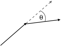
Figure 6: The angle $\theta$ is the basis for computing the curvature of the pair of black lines.

There are basically two ways to compute the term $|\kappa|^{p}$ from this angle: firstly, we can just take the power $p$ of the angle (which should be measured in arc length). The second method is based on the work of Bruckstein et al. Bruckstein-et-al-01 , and makes also use of the lengths $\ell(l_{1})$ and $\ell(l_{2})$ of the two lines:

$$\phantom{xxxx}\min\{\ell(l_{1}),\ell(l_{2})\}\left(\frac{\theta}{\min\{\ell(l_{1}),\ell(l_{2})\}}\right)^{p}\ \ .$$

The original idea of Bruckstein et al. was to take the longest straight lines pre- and succeeding a direction change. In our context we can only consider elementary boundary segments, so we do not have the same convergence properties. In practice we found that both weights work fine and Bruckstein et al’s weights significantly reduce the running time of the employed linear programming solver.

Denoting either of the two arising weights as $w_{l_{1},l_{2}}$, we get one of two components for the cost entry $c_{l_{1},l_{2}}$. Together with length regularity this entry is

$$\phantom{xxxx}c_{l_{1},l_{2}}=w_{l_{1},l_{2}}\,+\,\tfrac{1}{2}\big{(}\ell(l_{1})+\ell(l_{2})\big{)}\ \ .$$

There are however some special cases involving the image border, a point that we neglected in Schoenemann-Kahl-Cremers-09 : firstly, at the four corners of a rectangular domain $\Omega$ we will want to set the curvature weight to $0$. Note that we still penalize the angle in which a region boundary meets the domain boundary $\partial\Omega$.

A second point relates to the length weight: whenever one (or two) of the line segments in a pair is part of the domain border, its length should be set to $0$. Otherwise there would be a bias towards associating the regions at the image border to the background.

3.3 An Adequate Constraint System

As before for length regularity, the linear cost function (8) needs to be minimized subject to suitable constraints to closely reflect the discretized model function. In Schoenemann-Kahl-Cremers-09 we presented two sets of constraints, with the aim to ensure that the boundary variables indeed describe a boundary of the region variables. In this work we show that two more sets of constraints are needed, where the second one becomes necessary only when several regions meet in a single point. In particular, we will show that in this case there are several valid boundaries and that our method searches for the one with least cost.

Firstly, we adapt the surface continuation constraints to the new kind of boundary variables. To this end, we define the incidence $m_{e}^{l_{1},l_{2}}$ of a line segment pair and a boundary segment $e\in\mathcal{E}$. This value is defined as $0$ unless $l_{1}$ is an orientation of $e$ (note that $l_{2}$ is irrelevant for this value). Otherwise the value is the same as the previously defined incidence of $l_{1}$ and $e$. Hence, the surface continuation constraints read

$$\phantom{xxxx}\sum\limits_{f\in\mathcal{F}}m_{e}^{f}\,y_{R}^{f}\ =\ \sum\limits_{l_{1},l_{2}\in\mathcal{E}^{O}}m_{e}^{l_{1},l_{2}}\,y_{B}^{l_{1},l_{2}}\ \ \ \forall e\in\mathcal{E}\ \ .$$ (9)

These constraints alone leave a lot of freedom. In particular, we could choose line pairs without direction changes everywhere. What is really wanted, though, is that for every active $y_{b}^{l_{1},l_{2}}$ both $l_{1}$ and $l_{2}$ belong to the region boundary induced by the region variables. This is ensured by two sets of constraints, where the first is called boundary continuation. In words it can be stated as

Boundary Continuation Constraint: If a pair of line segments $l_{1},l_{2}$ is active, there must be a succeeding pair $l_{2},l_{3}$ that is also active. Likewise there must be a preceeding active pair $l_{0},l_{1}$.

These constraints ensure that the active line pairs actually define closed paths. They are identical to the constraints arising for the computation of shortest paths in a graph such as Amini-et-al-90 and are stated as

$$\sum\limits_{l_{0}}y_{B}^{l_{0},l_{1}}=\sum\limits_{l_{2}}y_{B}^{l_{1},l_{2}}\ \ \ \forall\,l_{1}\in\mathcal{E}^{O}\ \ .$$

Now we have paths, but we cannot guarantee that all parts of these paths are actually region boundaries. Indeed, we invite the reader to check that the configuration in Figure 7 (a) satisfies all constraints introduced so far. Moreover, for small length weights and squared curvature the cost of this configuration will be lower than those of the desired configuration shown in part (b).

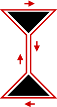
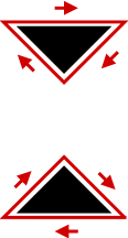
(a)	(b)

Figure 7: Without the boundary consistency constraints the configuration in (a) is valid and – for squared curvature and without length penalty– cheaper than the desired one in (b). With boundary consistency (b) remains feasible, but (a) is excluded, as desired.

To exclude cases such as (a) from the optimization, we add a new set of constraints:

Boundary Consistency Constraint: For every boundary segment, only one of the two possible orientations can be active.

To formalize this, we denote by $e^{\rightarrow}$ and $e^{\leftarrow}$ the positive and negative orientation of a boundary segment $e$. Then the constraint can be written as

$$\sum\limits_{l_{1}}y_{B}^{l_{1},e^{\leftarrow}}+\,\sum\limits_{l_{2}}y_{B}^{e^{\rightarrow},l_{2}}\leq 1\ \ \forall e\in\mathcal{E}\ \ .$$

Similar sets of constraints can be derived, e.g. $\sum_{l_{1}}y_{B}^{e^{\leftarrow},l_{1}}+\,\sum_{l_{2}}y_{B}^{l_{2},e^{\rightarrow}}\leq 1$, but experimentally we found them to be redundant. Moreover, if $e$ is part of the domain border $\partial\Omega$ then one of the orientations will never occur in a desired configuration. We simply disregard the corresponding variables.

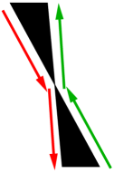
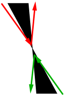
(a)	(b)	(c)

Figure 8: Determining boundaries is ambiguous: (a) A segmentation where two regions meet in a point. (b) A low-cost boundary configuration, where different pairs are indicated by different colors. (c) An equally valid, but more expensive boundary.

With these constraints, there is still one issue left to take care of, and it affects cases where several regions meet in a point. In this case, as shown in Figure 8, there are several valid boundary configurations. As long as only two regions meet, the given constraint system ensures that indeed the configuration with lower cost is selected. However, as soon as there are three or more regions meeting in a point, this constraint system will allow configurations with crossings, as exemplified in Figure 9. Should we really avoid such configurations? There is actually no obvious answer if one has in mind that, in the theory of continuous plane curves, the set enclosed by a positively oriented closed curve can be defined as the points of positive index (also called winding number) Rudin:1987 . In the example of Figure 9, the index of each point in a black triangle with respect to the outer curve defined by the arrows is one, so it makes sense to consider the curve as a region boundary . For the sake of comparison and completeness, we provide in section 6, Figure 13 a couple of experiments done either with or without crossing prevention. In the former case, we add a new set of constraints:

Crossing Prevention Constraint: If two pairs of line segments cross, only one of them may be active.

Denoting $\mathcal{C}$ the set of crossing line pairs, this constraint is easily formalized as

$$\phantom{xxxx}y_{B}^{l_{1},l_{2}}\,+\,y_{B}^{l_{3},l_{4}}\leq 1\ \ \ \forall(l_{1},l_{2},l_{3},l_{4})\in\mathcal{C}\ \ .$$

In practice these constraints are ignored in a first phase. Afterwards, the (usually very few) violated constraints are added in passes and the system is re-solved, until there are no more violated constraints. In our experiments we never needed more than $9$ passes. However, solving the arising programs can be quite time consuming, even when starting from the previous configuration.

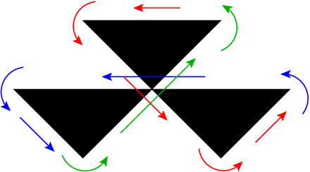
Figure 9: If three or more regions meet in a point, self-intersecting boundaries can define valid segmentations. If these are undesired, a fourth constraint set is needed. The different colors denote different phases when traversing the line. There is only one line.

In summary, region-based segmentation with curvature regularity is now expressed as the integer linear program

$$\min\limits_{\mathbf{y}_{R},\mathbf{y}_{B}} \mathbf{c}_{R}^{T}\,\mathbf{y}_{R}\ +\ \mathbf{c}_{B}^{T}\,\mathbf{y}_{B}$$

s.t. $$\sum\limits_{f\in\mathcal{F}}m_{e}^{f}\,y_{R}^{f}\ =\ \sum\limits_{l_{1},l_{2}\in\mathcal{E}^{O}}m_{e}^{l_{1},l_{2}}\,y_{B}^{l_{1},l_{2}}\ \ \ \forall e\in\mathcal{E}$$

$$\sum\limits_{l_{0}}y_{B}^{l_{0},l_{1}}=\sum\limits_{l_{2}}y_{B}^{l_{1},l_{2}}\ \ \ \forall l_{1}\in\mathcal{E}^{O}$$

$$\sum\limits_{l_{1}}y_{B}^{l_{1},e^{\leftarrow}}+\,\sum\limits_{l_{2}}y_{B}^{e^{\rightarrow},l_{2}}\leq 1\ \ \ \forall e\in\mathcal{E}$$

$$y_{R}^{f}\in\{0,1\}\ \forall f\in\mathcal{F},\ \,y_{B}^{l_{1},l_{2}}\in\{0,1\}\ \forall\,l_{1},l_{2}\in\mathcal{E}^{O}\,,$$

and the optional constraints

$$y_{B}^{l_{1},l_{2}}\,+\,y_{B}^{l_{3},l_{4}}\leq 1\ \ \ \forall(l_{1},l_{2},l_{3},l_{4})\in\mathcal{C}\ .$$

A first evaluation of this new scheme was given in Figure 1 on page 1 which shows that curvature regularity is better suited to ensure connected regions in the presence of long and thin objects. Note that the found solutions for curvature are generally not globally optimal. Details on the optimization scheme are given in Section 5 and more experiments will be given in Section 6. First, however, we discuss how to handle the problem of image inpainting.

4 Inpainting

In image inpainting we are given an image $I:\Omega\rightarrow I\!\!R$ together with a damaged region $\Omega_{d}\subset\Omega$. This damaged region can have arbitrarily many connected components and each of these can enclose holes. The task is to fill the damaged region with values that fit nicely with the values of $I$ outside the damaged region.

To this end, the above integer linear program is generalized to give a structured inpainting approach, where we consider the continuous model Masnou-Morel-98 ; Masnou-02 ; Chan-Kang-Shen-02

$$\min\limits_{u:\Omega\rightarrow\{0,1\}} \int\limits_{I_{l}}^{I_{u}}\int\limits_{C_{u,t}}|\kappa_{C_{u,t}}(\mathbf{x})|^{p}\,d\mathcal{H}^{1}(\mathbf{x})\,dt$$

$$\mbox{s.t. }u(\mathbf{x})=I(\mathbf{x})\ \ \forall\mathbf{x}\in\Omega\setminus\Omega_{d}\ \ ,$$

where $I_{l}$ and $I_{u}$ are the minimal and maximal intensities of $I$ along the border of the damaged region, $C_{u,t}=\{\mathbf{x}\,|\,u(\mathbf{x})=t\}$ is the set of level lines for level $t$ of $u(\cdot)$ and again $p>0$ is an exponent for curvature.

For the case of absolute curvature ($p=1$) and that $\Omega_{d}$ consists of singly-connected components (i.e. the components do not enclose holes), an efficient global optimization scheme was given in Masnou-Morel-98 ; Masnou-02 . We are interested in the more general problem of arbitrary domains and exponents $p>0$. In particular, $p=2$ is usually a better model.

4.1 Discretization

As before for image segmentation, our strategy is to discretize the model (4) by introducing basic regions and pairs of boundary segments. However, the regions are no longer limited to two labels: the intensity $u_{f}$ of region $f\in\mathcal{F}$ can be anywhere between $I_{l}$ and $I_{u}$. We follow the strategy in Masnou-Morel-98 ; Masnou-02 and consider only integral values inside this range. The result is a fully discrete labeling problem.

Naturally, one also needs to change the right-hand-side values of the inequality constraints. Moreover, for inpainting we always include the crossing prevention constraints since by definition level lines cannot cross.

To make sure that the boundary variables truly reflect level lines, it would be advisable to associate each basic region multiple variables, reflecting level sets. Then, there would be a binary variable $y_{f}^{k}$ for every integral value $I_{l}\leq k\leq I_{u}$ where a value of $1$ reflects that the intensity $u_{f}$ of the basic region is at least equal to $k$ (i.e. $u_{f}\geq k$). For $k^{\prime}>k$ this would naturally entail the constraints $y_{f}^{k^{\prime}}\geq y_{f}^{k}$. Moreover, there would be binary variables $y_{l_{1},l_{2}}^{k}$ that would be forced to be consistent with the level variables exactly as for binary segmentation.

This strategy is however not practicable for the domain sizes we want to address: the problem is way too large scale. Instead, we settle for one integral variable $y_{R}^{f}\in\{I_{l},\ldots,I_{u}\}$ for every region $f\in\mathcal{F}$, directly reflecting the intensity $u_{f}$ of the face. In addition, there are boundary variables reflecting the intensity differences between neighboring regions. Inside the damaged domain they can be restricted to values $y_{B}^{l_{1},l_{2}}\in[0,I_{u}-I_{l}]$. For the fixed part, we only consider basic regions that border on the damaged region. At their other borders the respective boundary variables can take values in $\{0,\ldots,I_{u}\}$. In practice it is advisable to first subtract the constant $I_{l}$ from the entire image (note that each connected component of $\Omega_{d}$ can be processed independently).

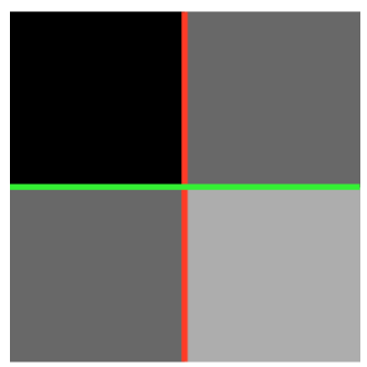
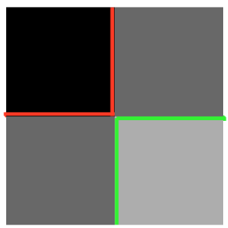
(a)	(b)

Figure 10: Best viewed in color. Estimated boundary variables for the given intensity profiles. Colors denote different pairs (not all pairs are shown) (a) With the proposed approximation we do not always get level lines. Here the boundary variables may jump between different intensity levels. (b) With level variables one would get the correct solution, but the computational demands are too high in practice.

As shown in Figure 10 this strategy does generally not give level lines, but it is a reasonable approximation. The arising integer linear program is stated as

$$\min\limits_{\mathbf{y}_{R},\mathbf{y}_{B}} \ \mathbf{c}_{B}^{T}\mathbf{y}_{B}$$

s.t. $$\sum\limits_{f\in\mathcal{F}}m_{e}^{f}\,y_{R}^{f}\ =\sum\limits_{l_{1},l_{2}\in\mathcal{E}^{O}}m_{e}^{l_{1},l_{2}}\,y_{B}^{l_{1},l_{2}}\ \ \ \forall e\in\mathcal{E}$$

$$\sum\limits_{l_{0}}y_{B}^{l_{0},l_{1}}=\sum\limits_{l_{2}}y_{B}^{l_{1},l_{2}}\ \ \ \forall l_{1}\in\mathcal{E}^{O}$$

$$\sum\limits_{l_{1}}y_{B}^{l_{1},e^{\leftarrow}}+\,\sum\limits_{l_{2}}y_{B}^{e^{\rightarrow},l_{2}}\leq I_{u}\ \ \ \forall e\in\mathcal{E}\$$

$$y_{B}^{l_{1},l_{2}}\,+\,y_{B}^{l_{3},l_{4}}\leq I_{u}\ \ \ \forall(l_{1},l_{2},l_{3},l_{4})\in\mathcal{C}$$

$$y_{R}^{f}=I_{f}-I_{l}\ \ \ \forall\,f\subset\Omega\setminus\Omega_{d}$$

$$y_{R}^{f}\in\{0,\ldots,I_{u}-I_{l}\}\ \ \ \ \forall\,f\subset\Omega_{d}$$

$$y_{B}^{l_{1},l_{2}}\in\{0,\ldots,I_{u}-I_{l}\}\ \ \ \ \forall\,l_{1},l_{2}\in\mathcal{E}^{O}\ \ .$$

Note that we have one such program for every connected component of $\Omega_{d}$.

4.2 Estimating Incoming Level Lines

A correct estimation of the direction of the level lines touching from outside the inpainting domain $\Omega$ is important, since the method aims at prolonging them with no additional curvature, if possible. We follow the simple and efficient method proposed by Bornemann and März in Bornemann-Maerz-07 after the work of Weickert Weickert-Book-98 ; Weickert-03 on the robust determination of coherence directions in image: at a point $x\in\Omega\setminus\Omega_{d}$, the coherence direction is the normalized eigenvector associated to the minimal eigenvalue of the structure tensor Bornemann-Maerz-07 :

$$\phantom{xxxx}J(x)=\frac{\Bigl{(}K_{\rho}\ast\Bigl{(}\mathds{1}_{\Omega\setminus\Omega_{d}}\nabla I_{\sigma}\otimes\nabla I_{\sigma}\Bigr{)}\Bigr{)}(x)}{\Bigl{(}K_{\rho}\ast\mathds{1}_{\Omega\setminus\Omega_{d}}\Bigr{)}(x)}$$ (12)

where $\mathds{1}_{\Omega\setminus\Omega_{d}}$ is the characteristic function of $\Omega\setminus\Omega_{d}$, $I_{\sigma}$ is defined as

$$\phantom{xxxx}I_{\sigma}=\frac{K_{\sigma}\ast\Bigl{(}\mathds{1}_{\Omega\setminus\Omega_{d}}I\Bigr{)}}{K_{\sigma}\ast\mathds{1}_{\Omega\setminus\Omega_{d}}},$$ (13)

and $K_{\rho}$, $K_{\sigma}$ are Gaussian smoothing kernels with standard deviations $\rho$ and $\sigma$. Experimentally, setting $\sigma=1.5$, $\rho=4$ yields a reliable estimation of the incoming level lines directions along $\partial\Omega_{d}$.

5 Optimization Strategies

In general, solving integer linear programs is an NP-hard problem Schrijver-Book-86 . In some cases, where there are linear inequality constraints $\mathbf{A}\mathbf{x}\leq\mathbf{b}$ and the matrix $\mathbf{A}$ is totally unimodular one can find the global optimum by solving the linear programming relaxation Schrijver-Book-86 , i.e. the problem one obtains when dropping all integrality constraints on the variables. For instance, a constraint $y_{i}\in\{0,1\}$ will be relaxed to $y_{i}\in[0,1]$. The arising problem can be solved in (weakly) polynomial time using interior point methods Ye-Book-97 .

Several of the discussed systems are in fact polynomial-time solvable, in particular the length-based problems and the boundary continuation constraints by themselves. The integer linear program for curvature regularity is however not in this class. Still, experimentally we found that solving the linear programming relaxation often gives nearly integral solutions. Moreover, the relaxation value provides a (usually quite tight) lower bound on the original problem. We proceed to discuss this strategy in detail.

5.1 Solving the Linear Programming Relaxation

There are two popular ways of solving general linear programs. Firstly, there is the dual simplex method Dantzig-Thapa-97 , based on refactorizing the constraint system. It is usually the most memory saving method and in practice superior to the primal simplex method. For some variants of the simplex method exponential worst-case run-times have been proved. On practical problems the method often works very well, and there are competitive and freely available implementations, e.g. the solver Clp. We found it quite useful for an 8-connectivity, but for a 16-connectivity – and very low length weights – we got acceptable running times only for some of the images we tried. In other cases the solver was terminated after several days without having solved the problem. In the end we chose the length weights high enough to get acceptable running times. The results we get indicate that these settings actually provide a very good model.

On the other hand, there are interior point methods which usually perform Newton-iterations on a primal-dual formulation of the problem. This entails frequent matrix inversions, solved via the sparse Cholesky decomposition. We are not aware of a freely available solver that performs well on large scale problems such as ours. Hence, we tested several commercial packages and found Gurobi and FICO Xpress to be well-suited solvers for our problem. Generally the running times of commercial interior point solvers are quite predictable. The downside is the memory consumption: we found that a little more than twice the memory consumption of a simplex solver is needed for our problem, where we tested with an 8- and a 16-connectivity.

For segmentation, the combination of licensing issues and the high memory demands made us use the simplex method. For inpainting, where the memory demands are lower, the interior point methods proved superior.

5.2 Obtaining and Evaluating Integral Solutions

Solving the linear programming relaxation provides a fractional solution as well as a lower bound on the original integral problem. Since the fractional solutions are often close to integral, we derive an integral solution by simply thresholding the region variables. This already defines a segmentation, but we would also like to know its energy, so we have to infer the associated boundary variables.

We already discussed the complications in case two or more regions meet in a point (see Section 3.3). Our method will then select the cheapest allowed boundary configuration according to the selected constraint set. In contrast, the recent method of El-Zehiry and Grady ElZehiry-Grady-10 will take the sum of all configurations here.

Due to these difficulties we so far did not implement a specialized routine to compute the energy of a segmentation, although this should be possible. Instead, we simply re-run the linear programming solver, this time with all region variables fixed according to the segmentation. Note that this strategy was also pursued in Schoenemann-Kahl-Cremers-09 , so the gaps reported there are w.r.t. the integer program, not the model itself.

In case crossing prevention was selected we again add violated constraints in passes. In addition, we fix all “impossible” boundary variables to $0$, where impossible refers to pairs of line segments where along one of the line segments the segmentation stays constant. In the vast majority of cases this produced an integral solution and hence the optimal boundary configuration. In a few cases we got up to $12$ fractional variables. We presently assume that the computed cost is close enough to the actual cost.

6 Experiments

In this section we evaluate the proposed scheme for both image segmentation and inpainting, where in all cases we consider the intensity range $[0,255]$. For image segmentation we also evaluate how close to the global optimum we got. The experiments were run on a 3.0 GHz Core2 Duo machine equipped with $8$ GB of memory. For segmentation we used the dual simplex method in the solver Clp, for inpainting we used the interior point method of Gurobi.

6.1 Image Segmentation

For binary image segmentation, we show experiments for a totally unsupervised problem and an interactive one where seed nodes are given.

Unsupervised Image Segmentation

For unsupervised image segmentation we use data functions $g_{0},g_{1}$ as in the piecewise constant functional of Mumford and Shah Mumford-Shah-89 , i.e. where the intensity of an image point is compared to the mean value of a region. This results in the model:

$$\int\limits_{\Omega}\!\!\Big{(}I(\mathbf{x})-\mu_{0}\Big{)}^{\!2}[1-u(\mathbf{x})]\,d\mathbf{x}\,+\int\limits_{\Omega}\!\!\Big{(}I(\mathbf{x})-\mu_{1}\Big{)}^{\!2}u(\mathbf{x})\,d\mathbf{x}$$

$$\hskip 28.45274pt+\,\nu\,|C|+\lambda\!\int\limits_{C}|\kappa_{C}(\mathbf{x})|^{2}\,d\mathcal{H}^{1}(\mathbf{x})\ \ \ .$$ (14)

We set the mean values $\mu_{0},\mu_{1}$ to the minimal and maximal intensity in the given image, respectively.

input	$\lambda=1000,\nu=10$	$\lambda=10000,\nu=10$	$\lambda=100000,\nu=10$
	within $0.75\%$.	within $3.6\%$.	within $4.4\%$.

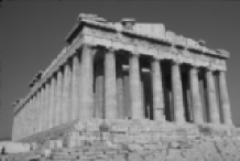
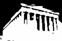
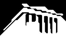
input	$\lambda=1000,\nu=10$	$\lambda=10000,\nu=10$	$\lambda=100000,\nu=10$
	within $0.6\%$.	within $2.8\%$.	within $3.6\%$.

Figure 11: Evaluation of the proposed method for unsupervised image segmentation and an 8-connectivity. Shown are segmentations for different curvature weights and how close they are to the lower bound (and hence the global optimum).

Figure 11 shows results of our method on images of size $128\times 128$ and $160\times 107$, respectively, using an 8-connectivity. Here we provide results for different curvature weights and it can be seen that even for very high weights long and thin structures are preserved. At the same time, the relative gap increases with the curvature weight.

These results took roughly $4$ hours computing time, where up to $9$ passes were needed. Though we re-used the existing solution, the first passes often took as long as solving the initial program.

Interactive Image Segmentation

Next we turn to the problem of interactive image segmentation for color images, where in addition to an image $I:\Omega\rightarrow I\!\!R^{3}$ we are given a set of foreground and background seed nodes as specified by a user. Since our focus is on evaluating the novel method, we did not refine the seed nodes. Hence, for each image the seed nodes were specified only once.

From the given seed nodes, we estimate normalized histograms of color values, resulting (after smoothing) in distributions $p_{F}(\cdot)$ and $p_{B}(\cdot)$ that are then used in the model:

$$-\int\limits_{\Omega}\!\log(p_{F}(I(\mathbf{x}))\,[1-u(\mathbf{x})]\,d\mathbf{x}\,$$ (15)

$$-\int\limits_{\Omega}\!\log(p_{B}(I(\mathbf{x}))\,u(\mathbf{x})\,d\mathbf{x}$$

$$\hskip 8.53581pt+\,\nu\,|C|+\lambda\!\int\limits_{C}|\kappa_{C}(\mathbf{x})|^{2}\,d\mathcal{H}^{1}(\mathbf{x})\ \ \ .$$ (16)

This function is minimized over all $u:\Omega\rightarrow[0,1]$ that are consistent with the seed nodes.

For the experiments, we use a $16$-connectivity and fix the ratio of the curvature weight $\lambda$ over the length weight $\nu$ to $20.0$. The presented results were then obtained within half a day and using between $6$ and $8$ GB of memory.

Figure 12 compares our results with a simple thresholding scheme and the length based method of Section 2. These results clearly show the tendency of length-based methods to suppress long and thin objects. With curvature regularity this is remedied.

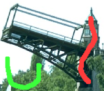
			within $0.5\%$.
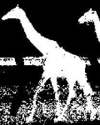
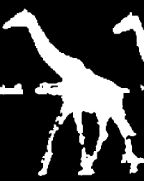
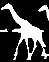
			global optimum
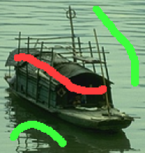
			within $2.6\%$.
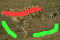
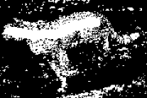
			within $2.2\%$.
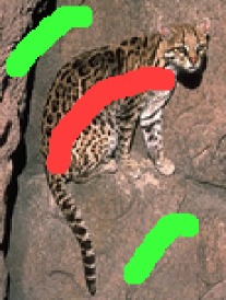
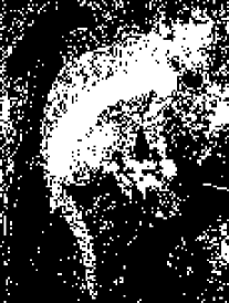
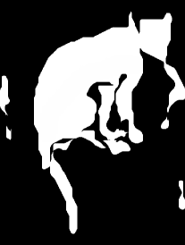
			within $1.5\%$.

Figure 12: Comparison of length-based and curvature-based methods. Left column: input images with seed nodes super-imposed. Middle left: thresholding scheme. Middle right: length-based segmentation (proposed method). In all cases $\lambda=1$. Right: length- and curvature-based segmentation (proposed method) and how close the results are to the global optimum. In all cases we set $\lambda=4$ and $\nu=0.2$. Images taken from the Berkeley database http://www.eecs.berkeley.edu/Research/Projects/CS/vision/grouping/segbench/.

Effects of the Constraint Sets

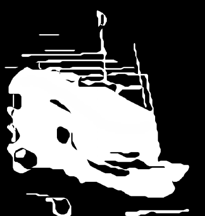
with crossing prevention	without crossing prevention
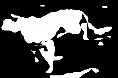
with crossing prevention	without crossing prevention

Figure 13: Without crossing prevention there is a bias towards triple points. For the top row significantly different segmentations are obtained with and without the constraints. For the bottom row there are only minor changes.

Above we indicated that it is debatable whether self-intersecting region boundaries should be allowed or not. In Figure 13 both possibilities are explored. For these images there were significant differences, for others, like the giraffe image, none at all. For the boat the results clearly improve when forbidding self-intersections, for the other image they grow slightly worse. In future work we hope to get closer to the respective global optima to find out which model is actually better.

Lastly, in this work we added the boundary consistency constraints to the original formulation in Schoenemann-Kahl-Cremers-09 . The latter formulation did in fact not represent the model correctly. Still, due to the relaxation adding the new constraints does not entirely solve the problem. When comparing the thresholded solutions of both versions we noticed as many changes to the good as to the bad. In future work we hope to improve on this.

6.2 Inpainting

We now turn to the problem of inpainting, where we use interior point solvers. Figures 14 and 15 show that our method is well-suited for structured inpainting, and that length regularity generally does not work well.

In this work we have improved upon our work Schoenemann-Kahl-Cremers-09 by previously estimating the direction of incoming level lines and giving a tighter constraint system. Figure 16 shows that these changes really improve the results.

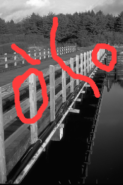
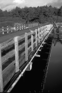
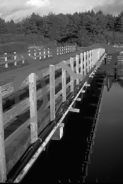
damaged image	inpainted with squared curvature	inpainted with length

Figure 14: For inpainting curvature is much better suited than length regularity.

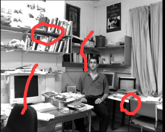
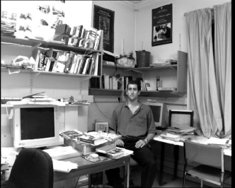
Figure 15: Our method applied to structured inpainting. Images taken from http://www.robots.ox.ac.uk/ vgg/data/data-various.html.

7 Conclusion

We have presented new theory and methods for length- and curvature-based regularization, both for image segmentation and inpainting. For curvature (in a region-based context) we are the first to propose a global approach in the sense that it is independent of initialization.

The results clearly demonstrate that curvature regularity outperforms length-regularity in the presence of long and thin objects. Experimentally we showed that for segmentation our strategy of solving a linear programming relaxation is usually within $5\%$ of the global optimum. In some cases it even finds the global optimum.

References

- [1] A.A. Amini, T.E. Weymouth, and R.C. Jain. Using dynamic programming for solving variational problems in vision. IEEE Transactions on Pattern Analysis and Machine Intelligence (PAMI), 12(9):855–867, September 1990.
- [2] M. Bertalmío, G. Sapiro, V. Caselles, and C. Ballester. Image inpainting. In ACM SIGGRAPH, July 2001.
- [3] A. Blake and A. Zissermann. Visual Reconstruction. MIT press, 1987.
- [4] F. Bornemann and T. März. Fast image inpainting based on coherence transport. Journal on Mathematical Imaging and Vision, 28(3):259–278, July 2007.
- [5] Y. Boykov and M.P. Jolly. Interactive graph cuts for optimal boundary and region segmentation of objects in n-d images. In IEEE International Conference on Computer Vision (ICCV), Vancouver, Canada, July 2001.
- [6] Y. Boykov and V.N. Kolmogorov. Computing geodesics and minimal surfaces via graph cuts. In IEEE International Conference on Computer Vision (ICCV), Nice, France, October 2003.
- [7] A.M. Bruckstein, A.N. Netravali, and T.J. Richardson. Epi-convergence of discrete elastica. Applicable Analysis, Bob Caroll Special Issue, 79:137–171, 2001.
- [8] T.F. Chan, S.H. Kang, and J. Shen. Euler’s elastica and curvature based inpaintings. SIAM Journal of Applied Mathematics, 2:564–592, 2002.
- [9] T.F. Chan and L. Vese. Active contours without edges. IEEE Transactions on Image Processing (TIP), 10(2):266–277, 2001.
- [10] G.B. Dantzig and M.N. Thapa. Linear Programming 1: Introduction. Springer Series in Operations Research. Springer, 1997.
- [11] N.Y. El-Zehiry and L. Grady. Fast global optimization of curvature. In IEEE Computer Society Conference on Computer Vision and Pattern Recognition (CVPR), San Francisco, California, June 2010.
- [12] S. Esedoglu and R. March. Segmentation with depth but without detecting junctions. Journal on Mathematical Imaging and Vision, 18:7–15, 2003.
- [13] L. Grady. Minimal surfaces extend shortest path segmentation methods to 3d. IEEE Transactions on Pattern Analysis and Machine Intelligence (PAMI), 32(2):321–334, February 2010.
- [14] D.M. Greig, B.T. Porteous, and A.H. Seheult. Exact maximum a posteriori estimation for binary images. Journal of the Royal Statistical Society, Series B, 51(2):271–279, 1989.
- [15] G. Kanizsa. Contours without gradients or cognitive contours. Italian Jour. Psych., 1:93–112, 1971.
- [16] M. Klodt, T. Schoenemann, K. Kolev, M. Schikora, and D. Cremers. An experimental comparison of discrete and continuous shape optimization methods. In European Conference on Computer Vision (ECCV), Marseille, France, October 2008.
- [17] S. Masnou. Disocclusion: A variational approach using level lines. IEEE Transactions on Image Processing (TIP), 11:68–76, 2002.
- [18] S. Masnou and J.M. Morel. Level-lines based disocclusion. In International Conference on Image Processing (ICIP), Chicago, Michigan, 1998.
- [19] D. Mumford and J. Shah. Optimal approximations by piecewise smooth functions and associated variational problems. Communications on Pure and Applied Mathematics, 42:577–685, 1989.
- [20] M. Nikolova, S. Esedoglu, and T. Chan. Algorithms for finding global minimizers of image segmentation and denoising models. SIAM Journal of Applied Mathematics, 66(5):1632–1648, 2006.
- [21] M. Nitzberg, D. Mumford, and T. Shiota. Filtering, segmentation and depth. In LNCS, volume 662. Springer Verlag, 1993.
- [22] P. Parent and S.W. Zucker. Trace inference, curvature consistency, and curve detection. IEEE Transactions on Pattern Analysis and Machine Intelligence (PAMI), 11(8):823–839, 1989.
- [23] W. Rudin. Real and complex analysis. McGraw-Hill, Inc., New York, NY, USA, 1987.
- [24] T. Schoenemann and D. Cremers. Introducing curvature into globally optimal image segmentation: Minimum ratio cycles on product graphs. In IEEE International Conference on Computer Vision (ICCV), Rio de Janeiro, Brazil, October 2007.
- [25] T. Schoenemann, F. Kahl, and D. Cremers. Curvature regularity for region-based image segmentation and inpainting: A linear programming relaxation. In IEEE International Conference on Computer Vision (ICCV), Kyoto, Japan, September 2009.
- [26] A. Schrijver. Theory of Linear and Integer Programming. Wiley-Interscience Series in Discrete Mathematics and Optimization. John Wiley & Sons, 1986.
- [27] J.M. Sullivan. A crystalline approximation theorem for hypersurfaces. PhD thesis, Princeton University, Princeton, New Jersey, 1992.
- [28] J.M. Sullivan. Computing hypersurfaces which minimize surface energy plus bulk energy. Motion by Mean Curvature and Related Topics, pages 186–197, 1994.
- [29] D. Tschumperlé. Fast anisotropic smoothing of multi-valued images using curvature-preserving PDE’s. International Journal on Computer Vision (IJCV), 68(1):65–82, June 2006.
- [30] J. Weickert. Anisotropic diffusion in image processing. Teubner, Stuttgart, 1998.
- [31] J. Weickert. Coherence-enhancing shock filters. In Pattern Recognition (Proc. DAGM), Magdeburg, Germany, September 2003.
- [32] Y. Ye. Interior Point Algorithms: Theory and Analysis. Wiley-Interscience series in discrete mathematics. John Wiley and Sons, 1997.