Local atom number fluctuations in quantum gases at finite temperature

Abstract

We investigate the number fluctuations in small cells of quantum gases pointing out important deviations from the thermodynamic limit fixed by the isothermal compressibility. Both quantum and thermal fluctuations in weakly as well as highly compressible fluids are considered. For the 2D superfluid Bose gas we find a significant quenching of fluctuations with respect to the thermodynamic limit, in agreement with recent experimental findings. An enhancement of the thermal fluctuations is instead predicted for the 2D dipolar superfluid Bose gas, which becomes dramatic when the size of the sample cell is of the order of the wavelength of the rotonic excitation induced by the interaction.

I Introduction

The experimental possibility of detecting few and even single atoms confined in magnetic or optical traps with high precision is opening new perspectives in the study of correlations WestbrookCorr ; Blochcorr and fluctuations Westbrook1D ; Esslinger ; Ketterle2010 ; Bouchoule ; Chin2010 ; Cornell2D in atomic and molecular gases at the mesoscopic and microscopic scale.

In the present work we investigate the fluctuations of the particle number in small sample cells of quantum gases, exploring the deviations from the predictions of thermodynamic theory which relates the fluctuations to the isothermal compressibility.

We consider two important examples of continuous systems. The first one is the ideal Fermi gas, a benchmark of statistical mechanics, which has been recently studied experimentally in atomic gases to point out the anti-bunching effect produced by the Pauli exclusion principle Esslinger ; Ketterle2010 . The second system is the dilute quasi-two dimensional (2D) bosonic gas in the superfluid regime. Two dimensional gases are particularly suited to measure the number fluctuations since one avoids the column density integration. Measurements of this kind have been recently carried out showing important quenching of the fluctuations in the degenerate regimeChin2010 , whose origin is clearly explained by our analysis. On the other hand quasi-2D Bose gases with dipolar interaction present an enhancement of number fluctuations. This is due to the roton-like spectrum Goraroton ; roton-like which has important consequences on the behaviour of the static structure factor, thus on the number fluctuations, especially at finite temperature.

When the size of the sample cell is large enough one can use the thermodynamic theory of fluctuations (see, e.g., LL5 ). The expression for particle number fluctuations at temperature $T$ reads

$$\langle\delta N^{2}\rangle=Nk_{B}Tn\kappa_{T},$$ (1)

which relates the fluctuations to the isothermal compressibility $\kappa_{T}=1/n^{2}\,\partial n/\partial\mu\equiv 1/nmc^{2}$, with $n$ the average density, $\mu$ the chemical potential and $c$ the speed of sound c . When $T$ is large the compressibility of the gas approaches the classical value $n\kappa_{T}=1/k_{B}T$ and one recovers the shot noise regime. An extension of the thermodynamic relation for the density fluctuations of non-uniform systems has been recently proposed as a tool to measure temperatures HoTerm . If the radius of the cell is not large enough, important deviations with respect to Eq. (1) start occurring. In our investigation we will mainly focus on the low temperature regime where quantum effects become particularly important.

The paper is organized as follows. In the next section we recall how to calculate the particle number fluctuations from the correlation function and the static structure factor, respectively. In section III we discuss the temperature dependence of fluctuations in a finite volume of an ideal Fermi gas in three dimensions. In the same section we also study the dependence of quantum fluctuations ($T=0$) on the shape of the probe volume. Then in section IV we analyse the density fluctuations for the case of an interacting quasi-2D Bose gas at temperatures far below the critical temperature. We condsider short-range interactions as well as long-range dipole-dipole interactions and discuss differences in the static structure factor and in the finite volume fluctuations. In the same section we provide an analytical expression – whose derivation for completeness is given in the Appendix – for the zero-temperature fluctuations in 2D and for a contact potential,

II Fluctuations in a finite volume

The particle number fluctuations $\langle\delta N^{2}\rangle$ in a finite cell of volume $V$ are calculated by double integration of the density-density correlation function $n\nu(|{\mathbf{r}}_{1}-{\mathbf{r}}_{2}|)=\langle n({\mathbf{r}}_{1})n({\mathbf{r}}_{2})\rangle-{n}^{2}$ over $V$ and can be written asSLS98 ; Astra2007

$$\langle\delta N^{2}\rangle=n\int\nu({\mathbf{r}})h({\mathbf{r}})d{\mathbf{r}}=n\int\!S({\mathbf{k}})H({\mathbf{k}})\frac{d{\mathbf{k}}}{(2\pi)^{D}},$$ (2)

where $D$ is the dimensionality of the system, $h({\mathbf{r}})=\int_{V}\int_{V}\delta({\mathbf{r}}_{1}-{\mathbf{r}}_{2}-{\mathbf{r}})d{\mathbf{r}}_{1}d{\mathbf{r}}_{2}$ is a geometrical factor which depends on the shape of the probe cell, $H({\mathbf{k}})=\int_{V}\int_{V}e^{i{\mathbf{k}}({\mathbf{r}}_{1}-{\mathbf{r}}_{2})}d{\mathbf{r}}_{1}d{\mathbf{r}}_{2}$ is its Fourier transform and $S({\mathbf{k}})=\int\nu({\mathbf{r}})e^{-i{\mathbf{k}}{\mathbf{r}}}d{\mathbf{r}}$ is the static structure factor. Geometrically $h({\bf r})$ corresponds to the volume of the overlapping region between a cell of volume $V$ and the same cell shifted by the vector ${\bf r}$. For large volumes (thermodynamic limit) $H({\bf k})\rightarrow V\delta({\bf k})$ and one finds $\langle\delta N^{2}\rangle=NS(k=0)$ yielding, at finite temperature, the thermodynamic expression Eq.(1). Deviations from the thermodynamic limit are directly related to the finite-$k$ behaviour of the static structure factor. In order to discuss these deviations it is useful to distinguish between weakly compressible and highly compressible fluids. Weakly compressible fluids are characterized by the condition $mc^{2}\geq E_{deg}$ where $E_{deg}\sim\hbar^{2}n^{2/D}/m$ is the degeneracy energy and include systems like the ideal Fermi gas, the unitary Fermi gas and superfluid Helium. For such systems the low temperature condition $k_{B}T\ll mc^{2}$ is easily reachable, yielding antibunching with respect to the shot noise limit, i.e., $\delta N^{2}<N$. Highly compressible fluids are instead characterized by the condition $mc^{2}\ll E_{deg}$. For such systems, which include dilute superfluid Bose gases, the low temperature condition $k_{B}T\ll mc^{2}$ is hardly reachable experimentally and the fluctuations naturally exhibit bunching effects with respect to the shot-noise limit. In the following we will consider two important examples: the ideal Fermi gas and the 2D Bose gas.

III Ideal Fermi Gas

As a paradigmatic example of weakly compressible fluids we consider the ideal Fermi gas, whose finite temperature density-density correlation function in three dimensions reads

$$\nu({\mathbf{r}})\!=\!\delta({\mathbf{r}})\!-\left[\frac{k_{B}T}{n\epsilon_{F}}\frac{k_{F}^{2}}{2\pi^{2}r}\int_{0}^{\infty}\!\!du\frac{u\sin\left(u\sqrt{\frac{k_{B}T}{\epsilon_{F}}}k_{F}r\right)}{e^{-\mu(T)/k_{B}T}\,e^{u^{2}}+1}\right]^{2},$$ (3)

where $k_{F}=(6\pi^{2}n)^{1/3}$ and $\epsilon_{F}=\hbar^{2}k_{F}^{2}/2m$ are the Fermi momentum and the Fermi energy, respectively. The chemical potential of the ideal Fermi gas $\mu(T)$ is obtained self-consistently from

$$\left(\frac{k_{B}T}{\epsilon_{F}}\right)^{3/2}\int_{0}^{\infty}\!\!du\frac{3u^{2}}{e^{-\mu(T)/k_{B}T}\,e^{u^{2}}+1}=1$$ (4)

Initially, we consider the particle number fluctuations in a spherical cell of radius $R$, for which the geometrical factor is

$$h(r)=\frac{4\pi R^{3}}{3}-\pi rR^{2}+\frac{\pi r^{3}}{12},$$ (5)

with $r\in[0,2R]$. In Fig. 1 we show $\langle\delta N^{2}\rangle$ as a function of temperature for $N=4/3\pi R^{3}n=100$ and $2000$ calculated from Eq. (2) (solid lines) and from Eq. (1) (dashed line). As expected the two results are the closer the larger the volume (and hence $N$) and, for finite volumes, they approach each other at large temperature when the deBroglie wavelength becomes smaller than the sample size. In particular the fluctuations in a finite volume are always larger then the ones predicted by the thermodynamic expression Eq. (1) and remain finite at $T=0$ where they have a purely quantum nature. In this limit, to the leading order in $N$, they can be written as Astra2007 ; Yvan ; Recati2010 $\langle\delta N^{2}\rangle\approx 3(3/(32\pi^{4}))^{1/3}N^{2/3}\ln(10.45N^{1/3})$. Such an expression suggests that quantum fluctuations have a surface nature being dominated by the dependence $N^{2/3}\propto R^{2}$. Let us also note that the approximation $\langle\delta N^{2}\rangle\approx nNk_{B}\kappa_{T=0}=3Nk_{B}T/(2\epsilon_{F})$ obtained by neglecting the $T$-dependence in the compressibility (see dashed-dotted line in Fig. 1), is bad for all $T$: at low temperatures quantum fluctuations are not taken into account and at large temperature the relation $\kappa_{T}\approx\kappa_{T=0}$ is not valid.

III.1 Surface shape dependence of quantum fluctuations

In order to get a better insight into the geometrical dependence of the quantum fluctuations Ketterle_private we calculate $\langle\delta N^{2}\rangle$ at $T=0$ for a cylinder with radius $R$ and length $L$, keeping the volume (and hence $N$) fixed. The particle number fluctuations are given by Eq. (2), with the geometrical factor

$$h(\rho,z)\!=\!(2L\!-\!z)\left[2R^{2}\arccos\left(\frac{\rho}{2R}\right)\!-\!\frac{\rho}{2}\sqrt{4R^{2}-\rho^{2}}\right],$$ (6)

where $z\in[0,2L]$ and $\rho\in[0,2R]$. The results are shown in the inset of Fig. 1 as a function of the aspect ratio $L/R$ and for $N=100$. We find that the particle number fluctuations are minimal for $L\simeq R$ where the surface is minimal and they are even smaller for a sphere with the same volume (horizontal dashed-dotted line). Interestingly, in the inset of Fig. 1 we also show that the result follows closely the dependence of the surface $S_{Cyl}=2V^{2/3}/\pi^{1/3}[2(L/R)^{1/3}+(R/L)^{2/3}]$ of the cylinder on the ratio $L/R$, for a fixed volume $V$. Deviations from the latter expression is due to the logarithmic term, which cannot be taken into account by the geometrical analysis.

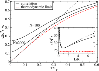
Figure 1: Number fluctuation $\langle\delta N^{2}\rangle$ for a free Fermi gas as a function of $T/T_{F}$ calculated integrating the density-density correlations (solid line) for $N=100$ and $N=2000$ and using the thermodynamic expression Eq. (1) (dashed line). Inset: $\langle\delta N^{2}\rangle$ at $T=0$ for a cylinder (solid line) and for a sphere (dashed-dotted line) for $N=100$ as a function of the aspect ratio $L/R$. The fluctuations closely follow the cylinder surface dependence (dashed line) for a fixed volume (see text).

IV 2D Bose gas with dipolar interaction

As important examples of highly compressible fluids we analyse dilute bosonic gases in the superfluid regime. Moreover we consider the system to be in a quasi-2D geometry where the motion along $z$ is frozen. This is usually realised with a strong harmonic confinement in the $z$ direction. We consider a quasi-2D gas, where the three dimensional $s$-wave scattering length $a$ is much smaller than the harmonic oscillator length $l_{z}$ in the $z$ direction. In this case it is possible to define an effective 2D short-range coupling constant $g=\hbar^{2}\sqrt{8\pi}a/(ml_{z})$. We will also include a long range dipole-dipole interaction, characterised by the parameter $g_{d}=2\sqrt{8\pi}d^{2}/(3l_{z})$, where $d$ is the dipole moment of the atom (or the molecule) which we take oriented perpendicular to the two dimensional plane of the gas.

Let us introduce the healing length $\xi=\hbar/(mc)$ and the chemical potential $\mu=mc^{2}=\hbar^{2}/(m\xi^{2})=g(1+\beta)n$, where $\beta=g_{d}/g=2md^{2}/(3\hbar^{2}a)$ is the ratio between of the dipole-dipole and the contact interaction strengthsFeshbach . Within Bogoliubov theory the spectrum of elementary excitations is roton-like

$$\frac{\epsilon(k)}{mc^{2}}=\xi k\sqrt{\frac{\xi^{2}k^{2}}{4}+1-\frac{\beta}{1+\beta}\frac{3}{2\sqrt{\pi}}F\left(\frac{kl_{z}}{\sqrt{2}}\right)},$$ (7)

with $F(x)=x\,\mathrm{erfc}\left(x\right)e^{x^{2}}$. In the absence of dipolar interaction ($\beta=0$) this spectrum has the well-known Bogoliubov form. For finite $\beta$ the dipolar term can significantly change the shape of the spectrum. For negative $s$-wave scattering length $a$ the spectrum can exhibit a roton-like minimum. Note, that in this case the gas must be stabilised against phonon instability, which demands $|\beta|>1$.

IV.1 Static structure factor

At low temperatures $T\ll T_{\lambda}$, where the gas is superfluid, the static structure factor $S(k,T)$ is related to the dispersion relation $\epsilon(k)$ of the elementary excitations via

$$S(k,T)=\frac{\hbar^{2}k^{2}}{2m\epsilon(k)}\coth\frac{\epsilon(k)}{2k_{B}T}.$$ (8)

The latter relation, Eq. (8), follows from the fact that the imaginary part of the response function in a weakly interacting Bose gas is $T$-independent and takes the form of a $\delta$-function BECbook .

The static structure factor depends significantly on the ratio $k_{B}T/(mc^{2})$. In Fig. 2 we show $S(k,T)$ as a function of $k\xi$ for different temperature with and without dipolar interaction. The peculiar roton-like shape of $\epsilon(k)$ shows up in a maximum in $S(k)$. This effect is significantly amplified at finite temperature as can be seen in Fig. 2. Actually, even if the spectrum does not exhibt a roton minimum (see the inset in the figure), a clear peak is visible in the static structure factor. Physically, this is due to thermal occupation of the roton-like states at finite $k$. The enhancement can be easily understood from Eq. (8) since, if $\epsilon(k)\ll k_{B}T$, the static form factor reduces to

$$S(k,T)\simeq S(k,0){2k_{B}T\over\epsilon(k)}={\hbar^{2}k^{2}k_{B}T\over m\epsilon(k)^{2}},$$ (9)

and in particular at low momenta we have $S(k,T)\simeq(1+Ak\xi)k_{B}T/(mc^{2})$ for $g_{d}\neq 0$, with $A=3\beta l_{z}/[\sqrt{8\pi}(1+\beta)]$ and $S(k,T)=(1-(k\xi/2)^{2})k_{B}T/(mc^{2})$ for $g_{d}=0$. It is worth noticing that the large thermal enhancement of the the structure factor near the roton minimimum is peculiar of dilute gases. In fact in a weakly compressible system, like superfluid helium the thermal energy $k_{B}T$ is always smaller than the roton energy. Moreover Bragg spectroscopy, a technique typically used to extract $S(k)$ in quantum gases, can only access the $T=0$ static structure factor, being sensitive to the imaginary part of the response function, rather than to the dynamic structure factor BECbook . We will show that the study of the particle number fluctuations can instead reveal the effect of the sizable temperature enhancement in $S(k)$ produced by the rotonic excitation.

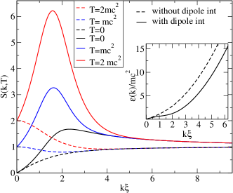
Figure 2: Static structure factor $S(k,T)$ for a quasi-2D Bose gas with (continuous lines) and without (dashed lines) dipolar interaction for $k_{B}T/mc^{2}=0$, $1$, $2$. Inset: the dispersion relation Eq. (7). For the dipolar case we use values for ⁵²Cr atoms, namely $a=-1.5a_{0}$, $l_{z}=0.09\mu m$ which corresponds to $\beta=-1.083$, $n/(\sqrt{2\pi}l_{z})=10^{14}$ cm^-3 and $\xi=2.5\mu$m.

IV.2 Fluctuations without dipolar interactions

First, we study the temperature dependence of the fluctuations in the non-dipolar case ($g_{d}=0$). In order to calculate the particle number fluctuations in a disk of radius $R$ we use Eq. (2) with the geometrical factor

$$H_{2D}(k)={4\pi^{2}R^{2}J_{1}^{2}(Rk)\over k^{2}},$$ (10)

where $J_{1}$ denotes the Bessel function. At $T=0$ the fluctuations can be calculated analytically (see appendix A)

$$\langle\delta N^{2}\rangle_{T=0}=\frac{\hbar^{2}}{mg}\frac{R}{\xi}\ln\left[C\frac{R}{\xi}\right],$$ (11)

with $C\approx 7.4$. The result for $\delta N^{2}$ as a function of temperature and for $N=12$, $100$ is shown in Fig. 3 where we also report the result (1), which holds in the thermodynamic limit. We used the parameters of the experiment reported in Ref. Chin2010 . In the inset we plot the fluctuations versus the interaction strength and compare with values measured in the superfluid regime of experiment Chin2010 . The agreement is pretty good. Further we show that the fluctuations are closer to the $T=0$ result Eq. (11) (dashed-dotted line) than to the thermodynamic limit. At finite $T$ we calculate the fluctuations using Eq. (8) with the dispersion relation Eq. (7) for $\beta=0$.

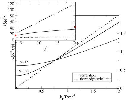
Figure 3: $\langle\delta N^{2}\rangle/N$ for a quasi-2D Bose gas in the superfluid regime as a function of $k_{B}T/(mc^{2})$ for $N=12$, $100$ and $g=\hbar^{2}/4m$, calculated from Eq. (2) (solid lines) and from Eq. (1) (dashed lines). Inset: $\langle\delta N^{2}\rangle$ as a function of the inverse of the dimensionless coupling constant $\bar{g}=mg/\hbar^{2}$ for $N=12$, $T=20nK$ calculated from Eq. (2) (solid lines) and from Eq.(1) (dashed lines). The (red) small boxes are the experimental value extracted from Chin2010 at $T\approx 20$nK. The $T=0$ result Eq. (11) is also reported for comparison (dashed-dotted line).

Fig. 3 shows that we have a significant deviation from the thermodynamic relation Eq. (1) at all temperatures. We can explain the behaviour of the fluctuation in an easy way within a simple approximation which describes how the fluctuations are related to the size of the sample cell. indeed if we consider a sphere of radius $R$ the relevant momenta contributing to the integral (2) are of the order $R^{-1}$ and the fluctuations can be approximated by the expression $\delta N^{2}\sim NS(\alpha/R,T)$, where $\alpha$ is a constant of order unity. There are three natural length scales in the problem: the healing length $\xi$, the phonon thermal wavelength $l_{p}=\hbar c/k_{B}T$ and the de Broglie wavelength $l_{T}=\hbar/\sqrt{mk_{B}T}$.

If $R\gg\xi$ the static structure factor reduces to

$$S\left(k\xi,\frac{k_{B}T}{mc^{2}}\right)\simeq{\alpha\xi\over{2R}}\coth\left(\frac{mc^{2}}{2k_{B}T}{\alpha\xi\over R}\right)={\alpha\xi\over{2R}}\coth\left({\alpha\over 2}{l_{p}\over R}\right),$$ (12)

and, as expected, only the phonon part of the spectrum plays a role. If the radius is also larger than the phonon thermal wavelength ($R\gg l_{p}$) we get, as expected LL5 , $\delta N^{2}=Nk_{B}T/mc^{2}$, i.e., we recover the thermodynamic result and, depending on the value of $T/mc^{2}$, the fluctuations can be sub- or super-poissonian. If, instead, $R\ll l_{p}$ we have $\delta N^{2}=\alpha N\xi/2R\propto N^{1/2}$, i.e., aside from the log-term, we recover the $T=0$ quantum result. Notice that the latter regime requires the condition $k_{B}T\ll mc^{2}$ and hence is difficult to access in dilute Bose gases.

In the opposite $R\ll\xi$ regime, we expect to probe the particle-like part of the spectrum. Indeed the static structure factor reads

$$\!S\!\left(k\xi,\frac{k_{B}T}{mc^{2}}\right)\!\simeq\coth\!\left[\frac{mc^{2}}{4k_{B}T}\!\left({\alpha\xi\over R}\!\right)^{2}\!\right]\!=\!\coth\!\left[\left(\alpha{l_{T}\over R}\right)^{2}\right].$$ (13)

Again we can distinguish two cases: for $R\gg l_{T}$, which is possible only for $k_{B}T\gg mc^{2}$, we get $\delta N^{2}=Nk_{B}T/mc^{2}(R/\xi)^{2}$, i.e., the fluctuations are reduced with respect to the thermodynamic limit, as clearly shown in Fig. 3 for $k_{B}T/mc^{2}>1$. If instead $R\ll l_{T}$, i.e. if $R$ is the smallest length scale of the problem, we recover the shot-noise result $\delta N^{2}=N$ which,by the way, coincides with the $T=0$ ideal Bose gas result.

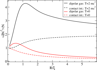
Figure 4: $\langle\delta N^{2}\rangle/N$ as a function of $R/\xi$ at zero temperature (dashed lines) and $k_{B}T/(mc^{2})=2$ (solid lines) for a dipolar gas of ⁵²Cr atoms (black lines) and for a non-dipolar gas $(\beta=0)$ (grey lines) with the same chemical potential. Parameters as in Fig. 2 and in particular $\xi=2.5\mu$m.

IV.3 Fluctuations with dipolar interactions

In order to calculate the particle number fluctuations in the presence of dipolar interactions $(g_{d}\neq 0)$ in a disk of radius $R$ we use again Eq. (2) with the geometrical factor 10. In the previous subsection we have seen that a discussion of the proper length scales can give a good estimation for the behaviour of the flutuations. For a dipolar gas there is another important length scale in the problem: $1/k_{max}$, which corresponds to the maximum of $S(k)$. Notice that even a small deviation of the excitation spectrum from the usual Bogoliubov form, without exhibiting a minimum (see inset in Fig. 2) leads to the maximum in $S(k)$, which is strongly amplified at finite $T$ as shown by Eq. (9). Hence, for sample cells of size $R\sim 1/k_{max}$ we expect, at finite $T$, a significant amplification of the particle number fluctuations. In Fig. 4, we report $\delta N^{2}$ calculated for a dipolar gas of ⁵²Cr atoms under experimentally feasible conditions Muller . Notice that the amplification of the fluctuations survive also for larger values of the cell size and the measurement of the particle number fluctuations is expected to provide a very sensitive tool to reveal the temperature amplification of the static structure factor in the rotonic-like region.

V Conclusion

We have shown that the investigation of the atom number fluctuations at the local scale provides a new insight on the microscopic structure of the correlations present in quantum gases where quantum and thermal effects combine in a non-trivial way. In particular, we explain the quenching of atom number fluctuations measured in a quasi-2D superfluid Bose gas Chin2010 . In a quasi-2D dipolar gas we obtain a crucial thermal enhancement of fluctuations. This opens new perspectives for future experimental investigations. The present analysis can be naturally extended to investigate also spin-fluctuations in quantum systems Recati2010 ; KetterleSpin .

A more quantitative comparison with experiments, where the cell $V$ has not sharp boundaries, would require the inclusion of the proper smooth weight function in the convolution integral Eq. (2).

Appendix A Zero temperature fluctuations of the 2D Bose-gas

In the present appendix we calculate analytically the particle number fluctuations at $T=0$ from Eq. (2) for a disk with radius $R$. Since the spectrum is given by Eq. (7) for $\beta=0$, and the geometrical factor by Eq. (10), the integral giving the number fluctuations can be written as

$$\langle\delta N^{2}\rangle=N\int_{0}^{\infty}dk\,\frac{J_{1}^{2}(Rk/\xi)}{\sqrt{1+\frac{k^{2}}{4}}}.$$ (14)

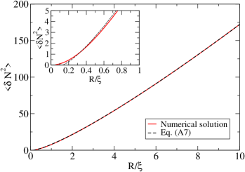
Figure 5: Comparison of $\langle\delta N^{2}\rangle$ as a function of $R/\xi$ for $\tilde{g}=1/4$ calculated numerically from Eq. (14) and Eq. (20). Inset: Zoom onto small $R/\xi$.

In order to get an analytical result we use the property of products of Bessel functions Eason1954 ; Watsonbook

$$J_{\eta+n}(A)J_{n}(B)=\frac{1}{\pi}\int_{0}^{\pi}d\theta\,\frac{J_{\eta}(X)}{X^{\eta}}\left(A-Be^{i\theta}\right)^{\eta}e^{-in\theta},$$ (15)

with $X^{2}=A^{2}+B^{2}-2AB\cos(\theta)$, which in our case reads

$$J^{2}_{1}(\tilde{R}k)=\frac{1}{\pi}\int_{0}^{\pi}d\theta\,J_{0}\left[2R/\xi k\sin\left(\frac{\theta}{2}\right)\right]e^{-i\theta}.$$ (16)

We introduce this in Eq. (14) and interchange the integrations

$$\langle\delta N^{2}\rangle=\frac{N}{\pi}\int_{0}^{\pi}d\theta\,F(\theta)e^{-i\theta}.$$ (17)

Then we are able to calculate the inner integral

$$F(\theta) \equiv 2\int_{0}^{\infty}dy\frac{J_{0}\left[4R/\xi\sin\left(\frac{\theta}{2}\right)y\right]}{\sqrt{1+y^{2}}}$$ (18)

$$=2\,I_{0}\left[2R/\xi\sin\left(\frac{\theta}{2}\right)y\right]\,K_{0}\left[2R/\xi\sin\left(\frac{\theta}{2}\right)y\right],$$

with the modified Bessel functions of zeroth order $I_{0}$ and $K_{0}$. In order to simplify the integral we split it at a small cutoff $\epsilon:=2\arcsin(\delta)$, with $\delta=(2R/\xi C_{1})^{-1}$ small for sufficiently large $R/\xi$. Here $C_{1}$ is an unknown numerical constant. The cutoff $\epsilon,\delta\ll 1$ is chosen such, that one can use the expansion of $I_{0}(z)K_{0}(z)\approx 1/(2z)$ (for large argument $z$) at $\theta>\epsilon$. The equation for the fluctuations simplifies to

$$\langle \delta N^{2}\rangle=\frac{2N}{\pi}\left\{\int_{\epsilon}^{\pi}d\theta\,\frac{e^{-i\theta}}{4R/\xi\sin\left(\frac{\theta}{2}\right)}\right.$$ (19)

$$\left.+\int_{0}^{\epsilon}d\theta\,e^{-i\theta}\,I_{0}\!\left[2R/\xi\sin\left(\frac{\theta}{2}\right)y\right]\,K_{0}\!\left[2R/\xi\sin\left(\frac{\theta}{2}\right)y\right]\!\right\}$$

One can show that the second integral vanishes for $\epsilon\ll 1$, in spite of the logarithmic divergence of $K_{0}$ at small arguments. Carrying out the first integral for $\epsilon,\delta\ll 1$ we finally obtain the particle number fluctuations

$$\langle\delta N^{2}\rangle=\frac{R/\xi}{\tilde{g}}\ln\left[CR/\xi\right],$$ (20)

with $C:=2C_{1}e^{-2+\ln 2}$. By numerically calculating the integral we find $C\approx 7.4$. This corresponds to $C_{1}\approx 13.7$ and thus $\delta\approx(27R/\xi)^{-1}$. Hence $\epsilon,\delta\ll 1$ is satisfied as long as $R/\xi\gg 0.04$. Fig. (5) compares Eq. (20) with the numerical solution of the integral in Eq. (14).

References

- (1) J. Esteve, J.-B. Trebbia, T. Schumm, A. Aspect, C. I. Westbrook, and I. Bouchoule, Phys. Rev. Lett. 96, 130403 (2006); T. Jeltes, J. M. McNamara, W. Hogervorst, W. Vassen, V. Krachmalnicoff, M. Schellekens, A. Perrin, H. Chang, D. Boiron, A. Aspect and C. I. Westbrook, Nature 445, 402 (2007).
- (2) S. Fölling, F. Gerbier1, A. Widera, O. Mandel, T. Gericke and I. Bloch, Nature 434, 481 (2005); T. Rom, Th. Best, D. van Oosten, U. Schneider, S. Fölling, B. Paredes and I. Bloch, Nature 444, 733 (2006).
- (3) M. Schellekens, R. Hoppeler, A. Perrin, J. Viana Gomes, D. Boiron, A. Aspect1 and C. I. Westbrook, Science 310, 648 (2005).
- (4) T. Müller, B. Zimmermann, J. Meineke, J.-P. Brantut, T. Esslinger, H. Moritz, Phys. Rev. Lett. 105, 040401 (2010).
- (5) C. Sanner, E. J. Su, A. Keshet, R. Gommers, Y. Shin, W. Huang and W. Ketterle, Phys. Rev. Lett. 105, 040402 (2010)
- (6) J. Armijo, T. Jacqmin, K. V. Kheruntsyan, and I. Bouchoule, Phys. Rev. Lett. 105, 230402 (2010). T. Jacqmin, J. Armijo, T. Berrada, K. V. Kheruntsyan, and I. Bouchoule, eprint: arXiv:1103.3028
- (7) C.-L. Hung, X. Zhang, N. Gemelke, and C. Chin, Nature 470, 236 (2011).
- (8) S. Tung et al., Phys. Rev. Lett. 105, 230408 (2010).
- (9) L. Santos, G. V. Shlyapnikov, and M. Lewenstein, Phys. Rev. Lett. 90, 250403 (2003).
- (10) M. Klawunn and L. Santos, Phys. Rev A 80, 013611 (2009).
- (11) E. M. Lifshitz, L. D. Landau, Statistical Physics, Part 1, Pergamon Press, 1980.
- (12) Here is the isothermal speed of sound which at low temperature is indistinguishable from the adiabatic one.
- (13) Q. Zhou and T.-L. Ho, eprint: arXiv: 0908.3015.
- (14) S. Giorgini, L. P. Pitaevskii, and S. Stringari, Phys. Rev. Lett. 80, 5040 (1998).
- (15) G. Astrakharchik, R. Combescot and L. P. Pitaevskii, Phys. Rev. A 76, 063616 (2007).
- (16) Y. Castin in Ultracold Fermi Gases, Proceedings of the International School of Physics Enrico Fermi, Course CLXIV ed. M. Inguscio, W. Ketterle, C. Salomon, (IOS Press, Amsterdam, 2008).
- (17) A. Recati and S. Stringari, Phys. Rev. Lett. 106, 080402 (2011).
- (18) We thank Wolfgang Ketterle for this interesting question.
- (19) L. Pitaevskii and S. Stringari, Bose-Einstein Condensation, Oxford Science Publications, Oxford (2003).
- (20) In this system the value of the scattering, and then , can be tuned by means of Feshbach resonance Cr-Fesh .
- (21) J. Werner et al., Phys. Rev. Lett. 94, 183201 (2005); T. Lahaye et al., Nature 448, 672 (2007); S. Müller et al., eprint: arXiv:1105.5015.
- (22) S. Müller, private communication.
- (23) C. Sanner et al., Phys. Rev. Lett. 106, 010402 (2011).
- (24) G. Eason, B. Noble and I. N. Sneddon, Phil. Trans. R. Soc. A 247, 529 (1955).
- (25) G.N. Watson, a treatise on the Theory of Bessel functions, Cambridge University Press, 1966.