Acceleration, magnetic fluctuations and cross-field transport of energetic electrons in a solar flare loop

Abstract

Plasma turbulence is thought to be associated with various physical processes involved in solar flares, including magnetic reconnection, particle acceleration and transport. Using Ramaty High Energy Solar Spectroscopic Imager (RHESSI) observations and the X-ray visibility analysis, we determine the spatial and spectral distributions of energetic electrons for a flare (GOES M3.7 class, April 14, 2002 23$:$55 UT), which was previously found to be consistent with a reconnection scenario. It is demonstrated that because of the high density plasma in the loop, electrons have to be continuously accelerated about the loop apex of length $\sim 2\times 10^{9}$cm and width $\sim 7\times 10^{8}$cm. Energy dependent transport of tens of keV electrons is observed to occur both along and across the guiding magnetic field of the loop. We show that the cross-field transport is consistent with the presence of magnetic turbulence in the loop, where electrons are accelerated, and estimate the magnitude of the field line diffusion coefficient for different phases of the flare. The energy density of magnetic fluctuations is calculated for given magnetic field correlation lengths and is larger than the energy density of the non-thermal electrons. The level of magnetic fluctuations peaks when the largest number of electrons is accelerated and is below detectability or absent at the decay phase. These hard X-ray observations provide the first observational evidence that magnetic turbulence governs the evolution of energetic electrons in a dense flaring loop and is suggestive of their turbulent acceleration.

1. Introduction

In the standard flare scenario, the magnetic energy stored in the solar corona is released accelerating particles. However, despite decades of effort, the exact mechanisms remain elusive. It is still unclear how and where exactly the particles are energized. Hard X-ray (HXR) imaging spacecrafts such as Yohkoh/HXT (Kosugi et al., 1991) and RHESSI (Lin et al., 2002) are particularly useful for the spatial and spectral diagnostics of energetic particles (Shibata, 1999; Aschwanden, 2002; Lin et al., 2003; Brown & Kontar, 2005; Lin, 2006; Temmer et al., 2010). Masuda et al. (1994, 1995); Sui et al. (2004); Liu et al. (2008); Joshi et al. (2009) have reported observations of a non-thermal HXR source above the top of an X-ray loop, suggesting coronal energy release via magnetic reconnection (see Priest & Forbes, 2002, as a review).

Along with magnetic reconnection, another important element of the standard flare model is magnetohydrodynamic (MHD) turbulence as it is believed to play a key role in a number of processes, from triggering fast reconnection to particle acceleration and transport. A considerable number of particle acceleration theories have been developed that require the presence of magnetic fluctuations in the flaring loop. Assuming a high level of MHD waves, it has been shown that stochastic acceleration can effectively accelerate a large number of both electrons and ions (Miller & Ramaty, 1987; Hamilton & Petrosian, 1992; Melrose, 1994; Miller et al., 1997; Petrosian & Bykov, 2008; Bykov & Fleishman, 2009; Bian et al., 2010; Petrosian & Chen, 2010). These particle acceleration models include both resonant and non-resonant interaction between the particles and various plasma waves. Waves and turbulence can be associated either with current sheets during magnetic reconnection (Chiueh & Zweibel, 1987; Somov & Kosugi, 1997; Litvinenko, 2006) or with reconnection outflows (Larosa et al., 1994). As the magnetic field in the solar corona is weak compared to the photosphere, direct measurement of even the mean field in the corona is problematic. Therefore, the fluctuating components of the coronal magnetic fields and their relation to energetic particles remain unknown. In addition, the location and physics of turbulent acceleration within the general picture of magnetic energy release is still awaiting an observational basis.

In this paper, using RHESSI X-ray observations and the visibility analysis technique, we show, for the first time, the presence of energy dependent cross-field transport of energetic electrons in a flaring loop. We estimate the relative magnitude and energy density of magnetic fluctuations which is required to explain these observations. We show that these HXR observations provide a quantitative basis for the turbulence measurements and its governing role in the evolution of energetic electrons and are suggestive of turbulent electron acceleration in this loop.

2. Lightcurves, spectra, and spatial distribution of X-rays from a flaring magnetic loop

We select a GOES M$3.7$ class flare, well-observed by RHESSI, which was previously analyzed by Sui et al. (2004); Veronig & Brown (2004); Bone et al. (2007); Xu et al. (2008). Sui et al. (2004) reported the existence of an X-ray source moving above the X-ray loop and concluded that the observations were consistent with the picture of the formation and development of a current sheet between the loop-top and coronal source. This April 14, 2002 $23:55$ UT flare (Figures 1-3) shows a simple loop structure over the whole duration of the flare and, importantly, the magnetic loop is filled with dense plasma $n\sim 10^{11}$cm^-3 (Veronig & Brown, 2004). Unlike the majority of solar flares, which typically produce the soft X-ray (SXR) emission in the coronal part of the loop and bright HXR emission in the dense chromospheric footpoints (e.g. Emslie et al., 2003; Kontar et al., 2008), the source of HXRs is coronal for this flare. Because of the high plasma density in the loop (Table 1), energetic electrons of $10-20$ keV are collisionally stopped in the coronal part of the loop and produce thick-target emission (Brown, 1971). At the same time, for such a dense loop, $20$ keV particles have collisional lifetime $\lesssim 0.1$s, so electrons need to be continuously accelerated in order to explain the observed HXR emission.

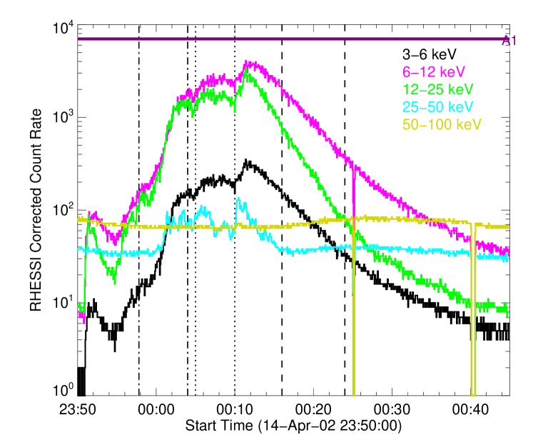
Figure 1.— Time profile in different RHESSI energy ranges of the 2002-04-14 event starting near 23:55 UT. The vertical lines indicates the three time periods for which the spectra, images and visibility forward fitting were performed.

We analyse this flare in three time intervals corresponding to the rise, peak and decay phases (see Fig 1). From the X-ray spectra (Fig 2), we determine the electron acceleration rate $dN/dt$ and the inverse power-law spectral index $\delta$ of non-thermal electrons, assuming a collisional thick-target model (Brown, 1971). We also obtain from an isothermal component in the spectral fit (Holman, 2005): the electron temperature $T_{e}$ and the emission measure of thermal plasma, i.e. $EM=n^{2}V$, where $n$ is the plasma density and $V$ is the volume occupied by the thermal plasma.

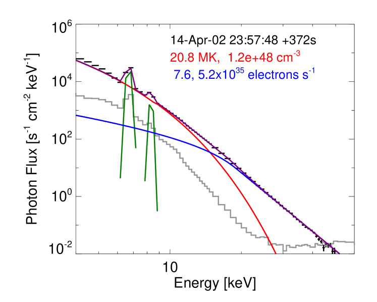
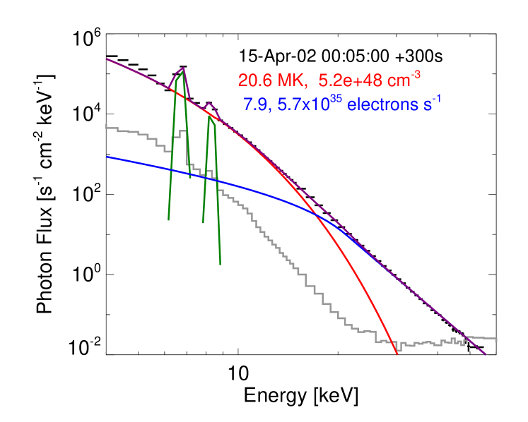
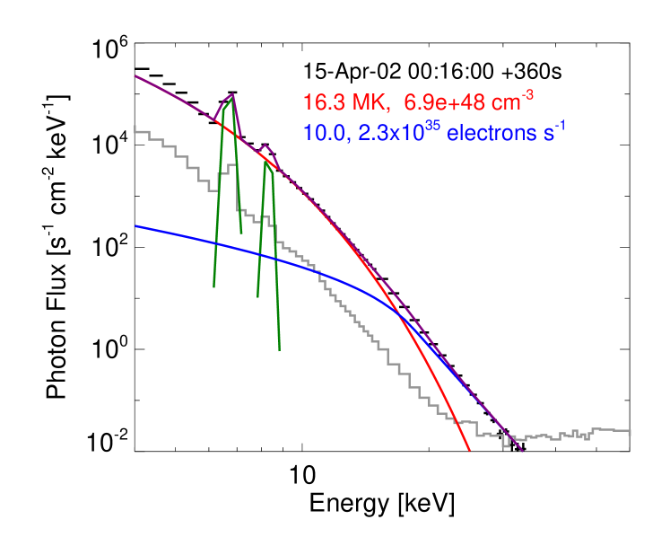
Figure 2.— The spatially integrated RHESSI X-ray spectra (black data points) for the three time intervals during the flare. These spectra were obtained using all front detectors excluding 2 and 7 (see Smith et al., 2002, for details) fitted (purple line) with an isothermal (red line) plus thick-target nonthermal (blue line) model. The pre-flare background spectra are shown in grey.

During the initial phase of the flare, acceleration of electrons up to $\sim 50$ keV is observed along with rapid heating of the plasma up to a temperature of $20$ MK (Fig 2). As the flare progresses, the thermal plasma emission measure grows while the temperature slightly increases reaching $23$ MK. The acceleration rate $dN/dt$ is found to be around $\sim 5\times 10^{35}$ electrons s^-1. In the decay phase of the flare, the thermal plasma starts to cool, the spectrum of energetic electrons steepens and the number of non-thermal electrons drops. The main flare parameters are summarized in Table 1.

Table 1HXR magnetic loop and flare parameters for the event starting April 14, 2002 23:55UT.

Time	$L(10\mbox{keV})$	$W(10\mbox{keV})$	$EM$	$T_{e}$	$V$ ($\pi W^{2}L/4$)	$n=\sqrt{EM/V}$	$\delta$	$dN/dt$	${\bf B}^{2}_{\perp}\lambda_{\parallel}/{\bf B}^{2}_{0}$
	(108cm)	(108cm)	(1048cm-3)	(MK)	(1026cm3)	(1010cm-3)		(1035 elec s-1)	(107cm)
23:57:48-00:04:00	20.3	4.8	1.2	21	1.4	9.3	7.3	5.2	2.3
00:05:00-00:10:00	22.0	7.5	5.2	20	3.7	11.8	7.8	5.7	2.3
00:16:00-00:24:00	23.5	11.2	6.9	16	8.9	8.8	9.8	2.3	$\lesssim$0.8

X-ray images reconstructed using the CLEAN algorithm (Hurford et al., 2002) for the three time intervals are presented in Figure 3. A clear loop structure is observed up to $\sim 20$ keV. Since RHESSI measures the spatial distribution of X-rays only indirectly, via rotating modulating collimators (Hurford et al., 2002), X-ray images can suffer from their reconstruction artifacts (Prato et al., 2009; Battaglia et al., 2011) and should not be used to determine the spatial size of the source. Instead, a more direct and hence reliable approach is to ‘stack’ the rotationally-modulated lightcurves over a number of spacecraft spin periods to produce X-ray visibilities (Hurford et al., 2002; Schmahl et al., 2007). The latter are instrument-independent 2-dimensional Fourier components of the HXR source (Schmahl et al., 2007). For a simple source geometry, as displayed in this flare, the position and sizes can be determined unambiguously at various energies. An additional advantage of the X-ray visibility fitting approach is that the statistical errors can easily be propagated to find the uncertainties associated with the inferred parameters of the loop (Kontar et al., 2008; Prato et al., 2009). Kontar et al. (2008, 2010) have successfully proved the robustness and sub-arcsecond precision of this method for HXR footpoints. X-ray visibilities are fitted using a curved elliptical gaussian model of the flare (Hannah et al., 2008; Xu et al., 2008). This is done for a number of energy ranges between $9$-$20$ keV and for the three time intervals (see Fig. 3). The Full Width Half Maximum (FWHM) source sizes, specifically the length $L(\epsilon)$, and width $W(\epsilon)$ and their corresponding statistical uncertainties, are obtained and presented in Figure 4. Using $L$ and $W$ at energy $10$ keV, we find the volume $V=\pi W^{2}L/4$ occupied by the thermal plasma. Assuming a volume filling factor of unity, the plasma density is calculated: $n=\sqrt{EM/V}$ (Table 1). It is found to be similar to the previous density estimates (Veronig & Brown, 2004; Bone et al., 2007; Xu et al., 2008).

As anticipated from the thick-target scenario in a weakly changing plasma density (see Brown et al., 2002, for details), the source length, $L(\epsilon)$, in the direction parallel to the guiding magnetic field, is a growing function of energy. The reason is that higher energy electrons can propagate further away from the region were they are accelerated, hence making the HXR source larger along the guiding field. In other words, in a dense coronal source, electrons travel a distance determined by their collisional losses. The stopping distance of an electron emitting X-rays of energy $\epsilon$ while moving along the guiding field of the loop is $r_{\parallel}\simeq\epsilon^{2}/(2Kn)$, where $K=2\pi e^{4}\ln\Lambda$, $e$ is the electron charge, $\ln\Lambda\simeq 20$ is Coulomb logarithm (Brown et al., 2002). For an energy independent length $L_{0}$ of the acceleration region, the FWHM length of the source is given by (Xu et al., 2008):

$$L(\epsilon)=L_{0}+\alpha_{\parallel}\epsilon^{2}.$$ (1)

By fitting Equation (1) to the measured $L(\epsilon)$, it is possible to determine $L_{0}$ and $\alpha_{\parallel}$ [arcsec keV^-2]. Figure 4 shows that the length of the acceleration region $L_{0}$ is around $\sim 2\times 10^{9}$ cm at the peak of the flare. Moreover, since $n=(2K\alpha_{\parallel})^{-1}$, $\alpha_{\parallel}$ can be used as an independent measure to determine the plasma density. This approach gives plasma densities of $9.8\times 10^{10}$cm^-3, $2.9\times 10^{11}$ cm^-3, $1.7\times 10^{11}$cm^-3 for the three time intervals analyzed in this paper. These densities are within a factor of two from the ones which were inferred above by using the thermal emission of the flare (see Table 1). Larger densities at the peak and decay phases of the flare can be attributed to the presence of a colder plasma invisible in Soft X-rays (SXR) with RHESSI, as suggested in previous studies of thermal sources (e.g. Jakimiec et al., 1998).

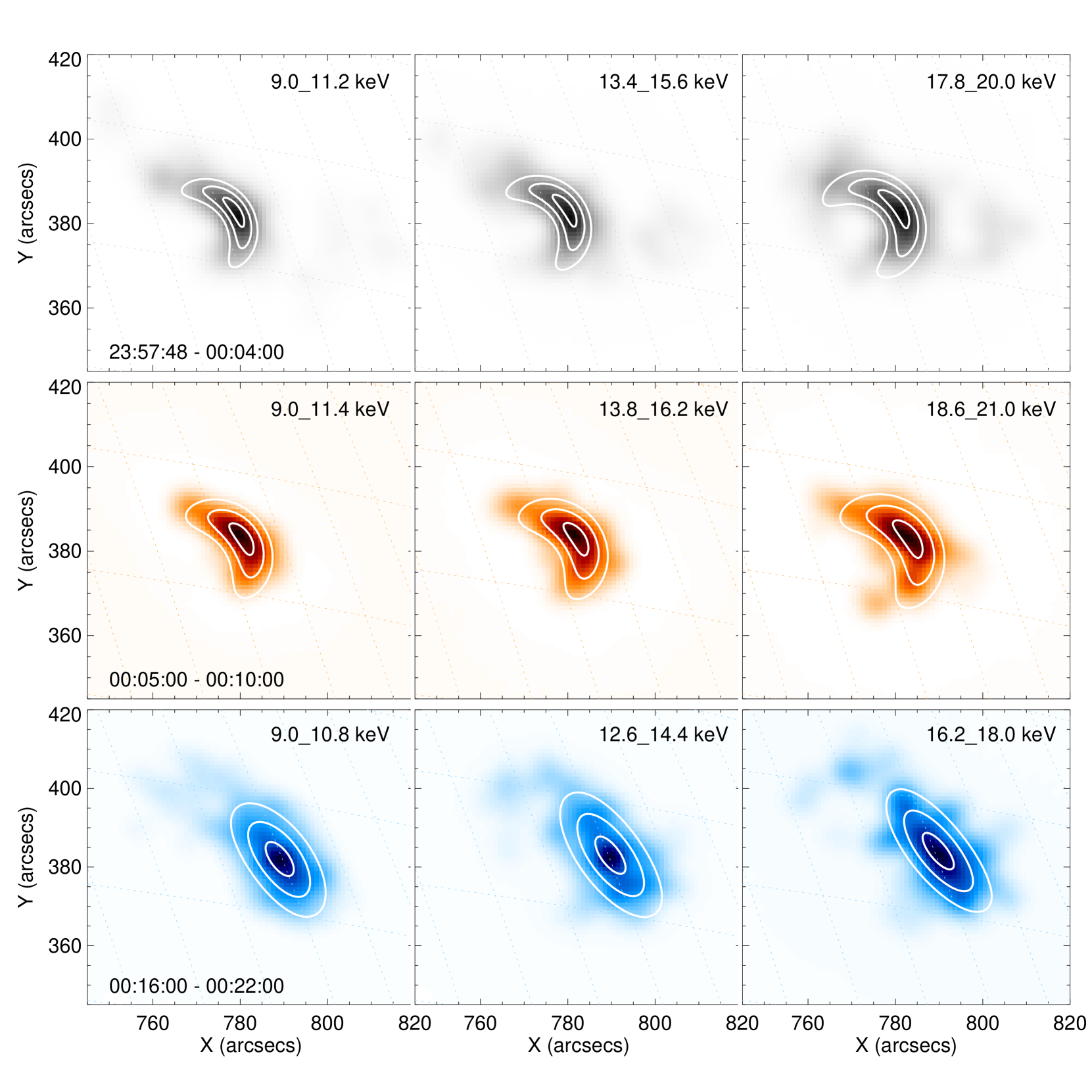
Figure 3.— CLEAN image overlayed by 30, 60 and 90% levels from the forward fitting to X-ray visibilities. Each row indicates a different time range. Each column a different energy range. The parameters of the loop are summarized in Table 1 and Figure 4.

3. Energy-dependent widths of the loop

The CLEAN images (Figs. 3) show that the loop width (size perpendicular to the guiding field) is like the length, growing with energy. This is seen quantitatively with the visibility forward fitted as a function of energy in Figure 4. A growing width $W(\epsilon)$ with energy is clearly present in the first and second time intervals (Figure 4) but could be absent in the third. This is particularly surprising as the guiding magnetic field is strong enough to ensure pure field-aligned transport of energetic electrons. Indeed, for a mean magnetic field of $\sim 150$ Gauss as measured in this loop using radio data (Bone et al., 2007), the Larmor radius of tens of keV electrons is $\sim 2$ cm and, therefore, the trajectories of their guiding centers coincide with the magnetic field lines. Collisions are unimportant in producing perpendicular transport for the parameters of the plasma, only resulting in a radial excursion (classical collisional diffusion) of the order of the electron gyroradius in a collisional time.

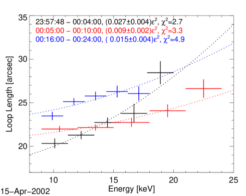
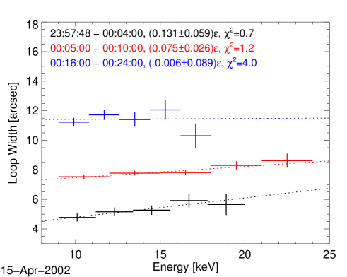
Figure 4.— The FWHM loop lengths (top) and widths (bottom) found from forward fitting the loop shape to the visibilities. The fitted lines are of the form $L(\epsilon)=L_{0}+\alpha_{\parallel}\epsilon^{2}$ and $W(\epsilon)=W_{0}+\alpha_{\perp}\epsilon$ for the lengths and widths respectively. The full $\chi^{2}$ quoted are calculated using the statistical uncertainties from X-ray visibility fits. $\alpha_{\perp}$ and $\alpha_{\parallel}$ are measured in units of [arcsec keV^-1] and [arcsec keV^-2] respectively.

However, it is well-known that particle transport across a mean magnetic field can be dramatically enhanced, well above the collisional value, in the presence of turbulence. The reason is the braiding of the field lines themselves due to perpendicular magnetic fluctuations. In the presence of magnetic fluctuations $\mathbf{B}_{\perp}$ perpendicular to the mean field $(\mathbf{B}_{0}=B_{0}\mathbf{z})$, perpendicular transport of field lines occurs which is governed by the following equation: ${d\mathbf{r_{\perp}}(z)}/{dz}={\mathbf{B_{\perp}}(\mathbf{r_{\perp}}(z),z)}/{B_{0}}$ (Rechester & Rosenbluth, 1978). Field lines braiding is believed to be a dominant process governing the transport of particles in the solar wind (Jokipii, 1966), in laboratory plasmas (Bickerton, 1997), and in thermal coronal loops (Galloway et al., 2006). It is safe to neglect the contribution of perpendicular electric fluctuations and subsequent $\mathbf{E}\times\mathbf{B}$ drift to cross-field transport. For MHD fluctuations, the electric field is $E_{\perp}\sim v_{A}B_{\perp}/c$ such that the magnetic drift $\mathbf{v}_{B}=v_{\parallel}(\mathbf{B}_{\perp}/B_{0})$ dominates over the electric drift $\mathbf{v}_{E}=c\mathbf{E}_{\perp}\times\mathbf{B}_{0}/B_{0}^{2}$ ($c$ is the speed of light and $v_{A}$ is the Alfven velocity). Since ${v}_{B}/{v}_{E}\sim v_{\parallel}/v_{A}$, the contribution of the $\mathbf{E}\times\mathbf{B}$ drift to perpendicular transport is negligible for non-thermal electrons with energies above $\gtrsim 10$ keV ($v_{\parallel}\simeq 6\times 10^{9}$ cm s^-1), i.e. $v_{\parallel}\gg v_{A}$, with $v_{A}\simeq 10^{8}$ cm s^-1 in the magnetic loop. The magnetic field line diffusion coefficient is given by the Taylor formula: $D_{M}=(1/B_{0}^{2})\int_{0}^{\infty}d\zeta<\mathbf{B_{\perp}}(\mathbf{r_{\perp}}(\zeta),\zeta)\mathbf{B_{\perp}}(\mathbf{r_{\perp}}(0),0)>$. Here, $<\mathbf{B}_{\perp}(\mathbf{r}_{\perp},z)\mathbf{B}_{\perp}(0,0)>$ is the two-points correlation function and $<>$ denotes an ensemble average. In the quasi-linear approximation, the perpendicular transport of field lines is characterized by a diffusion coefficient $D_{M}\simeq({B_{\perp}^{2}}/{B_{0}^{2}})\lambda_{\parallel}$, where $\lambda_{\parallel}$ is the parallel correlation length of the perturbations $\mathbf{B}_{\perp}$ (Jokipii & Parker, 1969; Rechester & Rosenbluth, 1978). An electron moves a distance $r_{\parallel}\simeq\epsilon^{2}/2Kn$ along the mean field in a collisional life-time. Therefore, this electron also makes a radial excursion given by $r_{\perp}=\sqrt{2D_{M}r_{\parallel}}$, as a consequence of the radial transport of field lines. This means that the FWHM width of the source $W(\epsilon)$ should also grow with energy. It is the sum of the acceleration region width $W_{0}$ and the diffusion part due to perpendicular transport:

$$W(\epsilon)=W_{0}+\alpha_{\perp}\epsilon,$$ (2)

where $\alpha_{\perp}=\sqrt{2D_{M}\alpha_{\parallel}}$ is measured in arcsec keV^-1. The unique feature of this expression is that it depends on the level of magnetic fluctuations via the magnetic field line diffusion coefficient $D_{M}$. Therefore, by measuring the energy dependent width of the flaring magnetic loop (Figure 4), we find automatically the diffusion coefficient for the magnetic field lines, i.e. $D_{M}=\lambda_{\parallel}{B_{\perp}^{2}}/{B_{0}^{2}}=\alpha_{\perp}^{2}/(2\alpha_{\parallel})$ (Table 1). As anticipated, $W(\epsilon)$ can be well fitted with a linear fit (Figure 4) to find $\alpha_{\perp}$ and the magnitude of magnetic fluctuations. The magnetic diffusion coefficient $\lambda_{\parallel}{B_{\perp}^{2}}/{B_{0}^{2}}$ is changing with time and is strongest when the acceleration rate $dN/dt$ of non-thermal electrons is at the maximum and the spectral index of the accelerated electrons is smaller (hardest HXR spectrum). The magnitude of fluctuations at the decay phase is weaker, so the data cannot provide a reliable estimate, but only an upper limit.

The energy density of magnetic fluctuations in the loop is $B_{\perp}^{2}/8\pi\simeq(B^{2}_{0}/8\pi)D_{M}/\lambda_{\parallel}$. Taking the length of the acceleration region $2\times 10^{9}$ cm as the upper limit for correlation length $\lambda_{\parallel}$, the energy density of magnetic fluctuations is $\simeq 10$ erg cm^-3 and the relative level of fluctuations $B_{\perp}/B_{0}\sim 0.1$. For $\lambda_{\parallel}=2.3\times 10^{7}$ cm, the magnetic perturbations follow to be strong $B_{\perp}/B_{0}=1$, and the energy density of turbulence $\simeq 900$ erg cm^-3. This value is close to the energy density of the flaring plasma $3nk_{B}T_{e}\simeq 830$ erg cm^-3 and much larger than the energy density of the non-thermal electrons

$$U_{nth}=\frac{1}{S}\int_{E_{c}}^{\infty}E\frac{F(E)}{\sqrt{2E/m_{e}}}\mbox{d}E,$$ (3)

where $S=\pi{W_{0}^{2}}/4$ is the cross-sectional area of the loop, $F(E>E_{c})\propto E^{-\delta}$ is the thick-target acceleration rate differential in energy [electrons s^-1 keV ^-1], and $E$ and $m_{e}$ are the electron energy and mass respectively. Using the values from thick-target fit and loop width measurements, the energy density of non-thermal electrons, $U_{nth}$ is about $11$, $6$, and $1$ erg cm^-3 for the three time intervals respectively. Therefore, we can conclude that the energy density of the magnetic turbulence is sufficient to energize at least non-thermal electrons and possibly the whole flare.

4. Discussion and conclusions

X-ray visibility based analysis has allowed us to infer the energy dependent source size for a well observed flaring loop. Both the length and the width of the loop are found to be larger at higher energies. This is in clear contrast with HXR footpoints, which show the opposite trend; higher energy sources appear smaller than lower energy sources (Kontar et al., 2008; Prato et al., 2009; Kontar et al., 2010). An energy dependent growth of the loop length is expected from the collisional precipitation of energetic electrons along field lines (Brown et al., 2002; Xu et al., 2008). The high density of the loop implies that the electrons are accelerated inside the loop region with the characteristic size $2\times 10^{9}$ cm. At the same time, the size of the loop perpendicular to the strong magnetic field is an increasing function of energy. The increase of the loop width implies strong cross-field transport of non-thermal electrons and is found to be consistent with the diffusion of magnetic field lines. This allows us to determine the level and locations of magnetic fluctuations in the flaring loop. For comparison, we note that the magnetic diffusion coefficient $D_{M}=\lambda_{\parallel}{B_{\perp}^{2}}/{B_{0}^{2}}$ measured in situ in the solar wind, where $B_{\perp}/B_{0}\sim 1$ and $\lambda_{\parallel}\sim 10^{11}$ cm (Matthaeus et al., 1986) is about four orders of magnitude larger than our values presented in Table 1.

We note that although the length and width of the flare are likely to be governed by parallel transport and diffusion of the magnetic field lines, equations (1,2) for the width and the length are approximations. The simultaneous treatment of acceleration, energy losses and cross-field transport is needed to assess the particle dynamics more accurately. This might lead to super or sub-diffusive cross-field transport of electrons and cannot be ruled out by the current data, so the radial excursions can scale as $r_{\perp}\propto\epsilon^{\beta}$, with $\beta$ close to one. Nevertheless, the width-energy measurements provide a powerful and unique tool to measure magnetic fluctuations in a flaring plasma. Importantly, the energy density of magnetic fluctuations appears to be energetically significant and is found to be larger than the energy density of non-thermal particles.

The temporal and spatial analysis by Sui et al. (2004) of the weaker source above the dense loop analyzed here suggests a picture consistent with formation of a reconnecting current sheet between the loop top and the coronal source. Assuming this reconnection scenario, our observations suggest the presence of MHD turbulence in the loop under the reconnection site. During the event, the length of acceleration site increases only by $\sim 10$%, while the width of the bright HXR loop $W_{0}$ grows with time more than a factor of $\sim 2$, which could be attributed to continuous piling up of newly reconnected lines. The plasma mode responsible for the perturbations remain unknown, but these observations indicate the presence of noticeable magnetic fluctuations during the solar flare inside the loop, where the acceleration of electrons is happening. It is possible to speculate that the magnetic field fluctuations are produced by magnetic reconnection above the loop and accelerate electrons inside the flaring loop.

References

- Aschwanden (2002) Aschwanden, M. J. 2002, Space Sci. Rev., 101, 1
- Battaglia et al. (2011) Battaglia, M., Kontar, E. P., & Hannah, I. G. 2011, A&A, 526, A3+
- Bian et al. (2010) Bian, N. H., Kontar, E. P., & Brown, J. C. 2010, A&A, 519, A114+
- Bickerton (1997) Bickerton, R. J. 1997, Plasma Physics and Controlled Fusion, 39, 339
- Bone et al. (2007) Bone, L., Brown, J. C., Fletcher, L., Veronig, A., & White, S. 2007, A&A, 466, 339
- Brown (1971) Brown, J. C. 1971, Sol. Phys., 18, 489
- Brown et al. (2002) Brown, J. C., Aschwanden, M. J., & Kontar, E. P. 2002, Sol. Phys., 210, 373
- Brown & Kontar (2005) Brown, J. C., & Kontar, E. P. 2005, Advances in Space Research, 35, 1675
- Bykov & Fleishman (2009) Bykov, A. M., & Fleishman, G. D. 2009, ApJ, 692, L45
- Chiueh & Zweibel (1987) Chiueh, T., & Zweibel, E. G. 1987, ApJ, 317, 900
- Emslie et al. (2003) Emslie, A. G., Kontar, E. P., Krucker, S., & Lin, R. P. 2003, ApJ, 595, L107
- Galloway et al. (2006) Galloway, R. K., Helander, P., & MacKinnon, A. L. 2006, ApJ, 646, 615
- Hamilton & Petrosian (1992) Hamilton, R. J., & Petrosian, V. 1992, ApJ, 398, 350
- Hannah et al. (2008) Hannah, I. G., Christe, S., Krucker, S., Hurford, G. J., Hudson, H. S., & Lin, R. P. 2008, ApJ, 677, 704
- Holman (2005) Holman, G. D. 2005, Advances in Space Research, 35, 1669
- Hurford et al. (2002) Hurford, G. J., Schmahl, E. J., Schwartz, R. A., et al. 2002, Sol. Phys., 210, 61
- Jakimiec et al. (1998) Jakimiec, J., Tomczak, M., Falewicz, R., Phillips, K. J. H., & Fludra, A. 1998, A&A, 334, 1112
- Jokipii (1966) Jokipii, J. R. 1966, ApJ, 146, 480
- Jokipii & Parker (1969) Jokipii, J. R., & Parker, E. N. 1969, ApJ, 155, 777
- Joshi et al. (2009) Joshi, B., Veronig, A., Cho, K., Bong, S., Somov, B. V., Moon, Y., Lee, J., Manoharan, P. K., & Kim, Y. 2009, ApJ, 706, 1438
- Kontar et al. (2010) Kontar, E. P., Hannah, I. G., Jeffrey, N. L. S., & Battaglia, M. 2010, ApJ, 717, 250
- Kontar et al. (2008) Kontar, E. P., Hannah, I. G., & MacKinnon, A. L. 2008, A&A, 489, L57
- Kosugi et al. (1991) Kosugi, T., Masuda, S., Makishima, K., Inda, M., Murakami, T., Dotani, T., Ogawara, Y., Sakao, T., Kai, K., & Nakajima, H. 1991, Sol. Phys., 136, 17
- Larosa et al. (1994) Larosa, T. N., Moore, R. L., & Shore, S. N. 1994, ApJ, 425, 856
- Lin (2006) Lin, R. P. 2006, Space Sci. Rev., 124, 233
- Lin et al. (2002) Lin, R. P., Dennis, B. R., Hurford, G. J., et al. 2002, Sol. Phys., 210, 3
- Lin et al. (2003) Lin, R. P., et al. 2003, Advances in Space Research, 32, 1001
- Litvinenko (2006) Litvinenko, Y. E. 2006, A&A, 452, 1069
- Liu et al. (2008) Liu, W., Petrosian, V., Dennis, B. R., & Jiang, Y. W. 2008, ApJ, 676, 704
- Masuda et al. (1995) Masuda, S., Kosugi, T., Hara, H., Sakao, T., Shibata, K., & Tsuneta, S. 1995, PASJ, 47, 677
- Masuda et al. (1994) Masuda, S., Kosugi, T., Hara, H., Tsuneta, S., & Ogawara, Y. 1994, Nature, 371, 495
- Matthaeus et al. (1986) Matthaeus, W. H., Goldstein, M. L., & King, J. H. 1986, J. Geophys. Res., 91, 59
- Melrose (1994) Melrose, D. B. 1994, ApJS, 90, 623
- Miller et al. (1997) Miller, J. A., Cargill, P. J., Emslie, A. G., Holman, G. D., Dennis, B. R., LaRosa, T. N., Winglee, R. M., Benka, S. G., & Tsuneta, S. 1997, J. Geophys. Res., 102, 14631
- Miller & Ramaty (1987) Miller, J. A., & Ramaty, R. 1987, Sol. Phys., 113, 195
- Petrosian & Bykov (2008) Petrosian, V., & Bykov, A. M. 2008, Space Sci. Rev., 134, 207
- Petrosian & Chen (2010) Petrosian, V., & Chen, Q. 2010, ApJ, 712, L131
- Prato et al. (2009) Prato, M., Emslie, A. G., Kontar, E. P., Massone, A. M., & Piana, M. 2009, ApJ, 706, 917
- Priest & Forbes (2002) Priest, E. R., & Forbes, T. G. 2002, A&A Rev., 10, 313
- Rechester & Rosenbluth (1978) Rechester, A. B., & Rosenbluth, M. N. 1978, Physical Review Letters, 40, 38
- Schmahl et al. (2007) Schmahl, E. J., Pernak, R. L., Hurford, G. J., Lee, J., & Bong, S. 2007, Sol. Phys., 240, 241
- Shibata (1999) Shibata, K. 1999, Ap&SS, 264, 129
- Smith et al. (2002) Smith, D. M., Lin, R. P., Turin, P., et al. 2002, Sol. Phys., 210, 33
- Somov & Kosugi (1997) Somov, B. V., & Kosugi, T. 1997, ApJ, 485, 859
- Sui et al. (2004) Sui, L., Holman, G. D., & Dennis, B. R. 2004, ApJ, 612, 546
- Temmer et al. (2010) Temmer, M., Veronig, A. M., Kontar, E. P., Krucker, S., & Vršnak, B. 2010, ApJ, 712, 1410
- Veronig & Brown (2004) Veronig, A. M., & Brown, J. C. 2004, ApJ, 603, L117
- Xu et al. (2008) Xu, Y., Emslie, A. G., & Hurford, G. J. 2008, ApJ, 673, 576