MAGNETIC-FIELD MEASUREMENTS OF T TAURI STARS IN THE ORION NEBULA CLUSTER

Abstract

We present an analysis of high-resolution ($R\sim 50,000$) infrared K-band echelle spectra of 14 T Tauri stars in the Orion Nebula Cluster. We model Zeeman broadening in three magnetically sensitive Ti I lines near $2.2\ \mu$m and consistently detect kilogauss-level magnetic fields in the stellar photospheres. The data are consistent in each case with the entire stellar surface being covered with magnetic fields, suggesting that magnetic pressure likely dominates over gas pressure in the photospheres of these stars. These very strong magnetic fields might themselves be responsible for the underproduction of X-ray emission of T Tauri stars relative to what is expected based on main-sequence star calibrations. We combine these results with previous measurements of 14 stars in Taurus and 5 stars in the TW Hydrae association to study the potential variation of magnetic-field properties during the first 10 million years of stellar evolution, finding a steady decline in total magnetic flux with age.

1 INTRODUCTION

T Tauri stars (TTSs) are a class of low-mass variable stars. Typically a few million years (Myr) old, TTSs have recently formed out of dense molecular cloud cores and are evolving toward the main sequence along their Hayashi tracks. These young solar-type stars display many spectral pecularities, often including excess continuum emission at ultraviolet through infrared (IR) wavelengths, strong and variable H$\alpha$ and Ca II H and K emission lines, both red- and blue-shifted absorption features in Balmer lines, and forbidden line emission. These spectral characteristics are most prominent in the spectra of so-called classical TTSs (CTTSs), which are TTSs still surrounded by dusty accretion disks. Another category of TTSs, naked TTSs (NTTSs), do not appear to have such disks around them and show little or no sign of accretion. For a comprehensive introduction to TTSs, readers are directed to recent reviews by Ménard & Bertout (1999) and Petrov (2003).

Stellar magnetic fields are thought to play an important role during the evolution of TTSs. Strong magnetic fields are believed to directly control the interaction between CTTSs and their circumstellar disks (e.g., Bouvier et al., 2007). Magnetic fields are thought to truncate the disks at or near the corotation radius, forcing disk material to accrete along the field lines onto the central star (Camenzind, 1990; Königl, 1991; Collier Cameron & Campbell, 1993; Shu et al., 1994; Paatz & Camenzind, 1996). While there is abundant evidence in support of this picture (Bouvier et al., 2007), observational detection of magnetic fields is difficult, and there remain relatively few magnetic field measurements on young stars.

The most successful approach thus far for measuring the total magnetic flux on cool stars has been measuring the Zeeman broadening of spectral lines in unpolarized light (Robinson, 1980; Saar, 1988; Valenti et al., 1995; Johns-Krull & Valenti, 1996; Johns-Krull et al., 1999b, 2004; Yang et al., 2005, 2008; Johns-Krull, 2007). For any given Zeeman component, the splitting resulting from the magnetic field is

$$\Delta\lambda\,[\textrm{m{\AA}}]={e\over 4\pi m_{e}c^{2}}\lambda^{2}gB=4.67\times 10^{-7}\lambda^{2}gB\ ,\,\,\,\,\,\,$$

where $g$ is the Landé $g$-factor of the transition, $B$ is the strength of the magnetic field in kG, and $\lambda$ is the wavelength of the transition in Å. Johns-Krull et al. (1999b, hereafter Paper I) detected Zeeman broadening of the Ti I line at $2.2233\ \mu$m on the CTTS BP Tau and obtained a field strength of $\bar{B}=2.6\pm 0.3$ kG averaged over the entire surface of the star. From the analysis of four Ti I lines near $2.2\ \mu$m, Johns-Krull et al. (2004, hereafter Paper II) measured a strong magnetic field of $2.5\pm 0.2$ kG on the NTTS Hubble 4. In addition to studying the Ti I lines, Paper II also examined several CO lines near $2.3\ \mu$m which have substantially reduced magnetic sensitivity and found no excess broadening beyond that due to stellar rotational and instrumental broadening.

Consistent detection of strong fields on TTSs raises the question of the origin of these fields. In the largest study to date of magnetic fields on TTSs, Johns-Krull (2007) used a sample of 14 stars to look for correlations between the measured magnetic-field properties and stellar properties that might be important for dynamo action. No significant correlations were found, and Johns-Krull (2007) speculated that the fields seen in these young stars may be entrained interstellar fields left over from the star formation process (e.g., Tayler, 1987; Moss, 2003). Yang et al. (2005, 2008, hereafter Papers III and IV) studied six TTSs in the TW Hydrae association (TWA). Roughly 10 Myr old (e.g., Barrado Y Navascués, 2006), the TWA stars are substantially older than the Taurus stars, whose age is $\sim$ 2 Myr (Palla & Stahler, 2000). Paper IV reported that the total unsigned magnetic flux of the stars appears to decrease with time from 2 Myr to 10 Myr, which further supports a primordial origin of the magnetic fields on TTSs.

In this work, we investigate the magnetic properties of TTSs in the Orion Nebula Cluster (ONC), which is even younger than the Taurus region. At a distance of $400$–$500$ pc (Hirota et al., 2007; Sandstrom et al., 2007; Jeffries, 2007), the ONC is one of the most extensively studied regions in the sky. Located just in front of the OMC-1 molecular cloud, it is the closest site of massive star formation. The age of the ONC is estimated to be $\sim$ 1 Myr by comparing the observed HR diagram with theoretical pre-main sequence evolutionary tracks (Hillenbrand, 1997). Strong ionizing radiation, primarily from the young and bright O6 star $\theta^{1}$ Ori C, evaporates the surrounding molecular gas, creating a huge cavity and exciting the famous Orion Nebula. Though much of this region still suffers strong extinction (e.g., Carpenter et al., 2001), a few thousand low-mass stars and brown dwarfs are visible in the optical. The young stars in the ONC provide an important sample for studies such as of the initial mass function of stellar clusters, the properties of circumstellar disks, and the evolutionary effects of high-mass stars on low-mass star formation. The dynamic star-formation activity in the ONC gives rise to strong stellar jets and outflows, resulting in violent interactions with the ambient molecular environment on various scales (e.g., Bally et al., 2000). O’dell (2001) gives a comprehensive review of this region.

In this paper, we report magnetic-field measurements for 14 TTSs in the ONC that allow the first investigation of the magnetic properties of TTSs in this region. In § 2, we describe the observations and data reduction procedures. In § 3, we present our analysis technique and the magnetic measurements. A discussion of our results is given in § 4, followed by our conclusions in § 5.

2 OBSERVATIONS

We conducted our observations on UT December 10–11, 2006, with the Phoenix high-resolution near-IR spectrometer (Hinkle et al., 2003) on the 8.1 m Gemini South Telescope at Cerro Pachon, Chile (program ID: GS-2006B-C-8). With the K4484 order-sorting filter, the grating was oriented to provide wavelength coverage between $2.2190$ and $2.2285\ \mu$m in air. This configuration allowed the recorded spectra to contain three magnetically sensitive Ti I lines as well as less magnetically sensitive lines of Fe I and Sc I. The 0$\farcs$34 (4-pixel) wide slit was used to achieve a spectral resolving power of $R\equiv\lambda/\delta\lambda\sim 50,000$. For each star, two exposures were acquired in nodding mode with an offset of 5″ along the 14″ long slit. Typical seeing was around 0$\farcs$5. Telluric and spectral standards were also observed each night. For data reduction, we used custom IDL software developed in Paper I that was originally written to handle data from the CSHELL (Tokunaga et al., 1990; Greene et al., 1993) spectrometer at the NASA Infrared Telescope Facility. The reduction procedures are described in Paper I and required minimal modification to work with the Phoenix data format. Seven strong telluric absorption lines were used for wavelength calibration. A summary of the ONC star observations is provided in Table 1.

Table 1: Journal of Observations

Object	R.A. (2000)	Dec. (2000)	UT Date	UT Time	Total Exposure Time (s)
2MASS 05353126-0518559	05:35:31.26	-05:24:18.4	2006 Dec 10	01:56	1200
V1227 Ori	05:35:10.58	-05:21:56.2	2006 Dec 10	02:40	1600
2MASS 05351281-0520436	05:35:12.81	-05:20:43.6	2006 Dec 10	03:16	1800
V1123 Ori	05:35:23.44	-05:10:51.7	2006 Dec 10	03:56	2280
OV Ori	05:35:52.76	-05:12:59.0	2006 Dec 10	04:44	2600
V1348 Ori	05:35:30.42	-05:25:38.5	2006 Dec 10	05:50	2880
LO Ori	05:35:08.22	-05:37:04.7	2006 Dec 10	06:49	2880
V568 Ori	05:35:36.44	-05:34:11.1	2006 Dec 10	07:45	3000
LW Ori	05:35:12.20	-05:30:32.9	2006 Dec 11	01:44	3600
V1735 Ori	05:35:22.45	-05:09:11.0	2006 Dec 11	02:53	3600
V1568 Ori	05:35:36.70	-05:37:41.5	2006 Dec 11	04:03	3600
2MASS 05361049-0519449	05:36:10.49	-05:19:44.9	2006 Dec 11	06:35	3600
2MASS 05350475-0526380	05:35:04.75	-05:26:38.0	2006 Dec 11	05:15	3600
V1124 Ori	05:35:47.39	-05:13:18.5	2006 Dec 11	07:46	3600

3 ANALYSIS AND RESULTS

We analyze three Ti I lines at 2.2211, 2.2233, and 2.2274 $\mu$m using the same procedures that are described in detail in Papers I–IV. The effective Landè g-factors of the three lines are 2.08, 1.66 and 1.58, respectively. First, for our objects, we obtain estimates of the stellar parameters $T_{\rm eff}$, $\log g$, and $v\sin i$ from the literature. Then we construct model atmospheres appropriate for the stars and calculate synthetic spectra. We predict the line profiles with no magnetic broadening and model the observed excess broadening to measure the surface magnetic fields on the TTSs in Orion. In contrast to our analysis of the stars in Papers III and IV, we do not have magnetically insensitive CO data to help verify the accuracy of the atmospheric parameters. However, two Fe I lines at 2.2257 and 2.2260 $\mu$m and one Sc I line at 2.2267 $\mu$m are available. These three lines have weak sensitivity to magnetic fields with effective Landè g-factors of 1.00, 0.74, and 0.50, respectively. So they essentially serve the same purpose as the CO lines (i.e., they help ensure that the excess broadening seen in the Ti I lines is magnetic in origin). These three lines are included in the fitting.

In order to construct appropriate model atmospheres, we obtain stellar atmospheric parameters from Hillenbrand (1997). We convert Hillenbrand (1997) spectral types to $T_{\rm eff}$ according to the relation provided in Johnson (1966). In a few cases, marked in the $T_{\rm eff}$ column in Table 2, we adjust $T_{\rm eff}$ by 100 or 200 K so that the predicted spectrum better matches the Fe I and Sc I lines. To calculate $\log g$, we use the stellar luminosities and masses from Hillenbrand (1997) and the $T_{\rm eff}$ converted from spectral types. Because of their youth, many of our objects have surface gravities lower than $3.5$ on the logarithmic scale, which is the lowest available in the NextGen Model Atmospheres grid (Allard & Hauschildt, 1995). In such cases, in order to avoid extrapolating the model atmosphere grid, we use $\log g$ = $3.5$. We expect that doing so produces only a modest ($\sim 10\%$) error in our measurements of magnetic fields, because our analysis technique is not very sensitive to small errors in $T_{\rm eff}$ or $\log g$, as shown by the extensive Monté Carlo analysis in Paper III. The $\log g$ values we derive from the Hillenbrand paper and those actually used in the analysis are listed along with other important stellar quantities in Table 2.

Table 2: Stellar Parameters

ID	Object		Spectral Type	$T_{\rm eff}$	$\log g_{H}$	$\log g$	$v\sin i$	$\log L_{bol}$	$M_{*}$	$R_{*}$	$P_{rot}$	Age
				(K)			(km s-1)	($L_{\odot}$)	($M_{\odot}$)	($R_{\odot}$)	(days)	($10^{6}$ yr)
867	2MASS 05353126-0518559	CTTS	K8	3900	2.98	3.50	11.5$\pm$1.0	0.249	0.30	2.93	10.66	0.7
347	V1227 Ori	CTTS	K5-K6	4200	3.33	3.50	10.0$\pm$0.8	0.086	0.41	1.72	7.33	3.4
391	2MASS 05351281-0520436	CTTS	M1	3500	3.27	3.50	10.6$\pm$1.5	-0.165	0.29	2.26	16.33	1.1
731	V1123 Ori	NTTS	M0/K8	3800	3.20	3.50	16.4$\pm$0.8	0.098	0.35	2.59	7.64	0.8
1021	OV Ori	CTTS	K5-K6	4000	3.62	3.62	14.0$\pm$1.8	0.105	0.63	2.36	N/A	1.3
850	V1348 Ori	CTTS	K8	3800	3.47	3.50	15.5$\pm$1.3	-0.107	0.40	2.04	7.78	1.3
321	LO Ori	CTTS	M0	3900	3.49	3.50	12.5$\pm$1.7	-0.195	0.38	1.75	7.74	2.0
923	V568 Ori	CTTS	M1	3664	3.25	3.50	6.2$\pm$1.9	-0.192	0.29	2.00	1.15	1.3
381	LW Ori	CTTS	M0.5	3800	3.32	3.50	15.9$\pm$1.2	-0.150	0.32	1.95	16.20	1.4
705	V1735 Ori	NTTS	K4	4400	N/A	4.00	16.6$\pm$0.8	N/A	N/A	N/A	N/A	N/A
926	V1568 Ori	NTTS	K7	4000	3.29	3.50	15.0$\pm$1.0	0.111	0.40	2.37	5.54	1.3
5073	2MASS 05361049-0519449	CTTS	K3	4200	3.97	4.00	9.2$\pm$1.2	0.191	1.14	2.35	N/A	1.4
258	2MASS 05350475-0526380	CTTS	M0.5	3664	3.34	3.50	10.4$\pm$1.0	-0.157	0.33	2.08	10.98	1.2
995	V1124 Ori	NTTS	M1.5	3589	3.17	3.50	6.2$\pm$1.3	-0.162	0.26	2.15	8.18	1.2

The magnetic models we use for the ONC stars are constructed in the same way as models 1–3 for the TWA stars in Paper IV, where they are fully described. Briefly, the stellar surface is treated as being composed of several regions. Each region has a filling factor (i.e., a fractional size) and is covered with a single magnetic field strength. The sum of all filling factors must be unity. All the models used here include a field-free region ($B=0$); however, Papers I and II show that generally the data do not demand the models have such a field-free region on the stellar surface. We also assume that these regions are spatially well mixed over the surface of the star. Models 1, 2, and 3 allow one, two, and three magnetic regions on the stellar surface, respectively, in addition to the field-free region. For models 1 and 2, the field strengths are free parameters. For model 3, we have field strengths in the three magnetic regions fixed at 2 kG, 4 kG, and 6 kG and fit only for the filling factor of each region. The mean magnetic field is just the sum of the field strengths ($B_{i}$) in the magnetic regions weighted by their corresponding filling factors ($f_{i}$), i.e., $\bar{B}=\displaystyle\sum_{i=1}^{n}B_{i}f_{i}$, where $n$ is the number of magnetic regions on the stellar surface in each model.

To compute the model spectrum for a star, we first interpolate the NextGen Model Atmosphere grid to the appropriate $T_{\rm eff}$ and $\log g$ and construct a model atmosphere specific for each star. Then we compute the spectrum for each magnetic-field region using the model atmosphere and a polarized radiative transfer code (Piskunov, 1999) that assumes a radial magnetic geometry in the stellar photosphere. We add in rotational broadening to the line profiles according to the $v\sin i$ of the star and convolve the resulting profiles with a Gaussian function corresponding to the observed spectral resolution ($50,000$). The spectrum for each region is then weighted by its filling factor and summed to form the final model spectrum. We use the nonlinear least-squares technique of Marquardt (Bevington & Robinson, 1992) and solve for the combination of field strengths and filling factors that yields the best fit to the observed spectrum.

The majority of our objects are CTTSs and are subject to substantial K-band veiling. Veiling is an excess continuum source, presumably from the circumstellar disk, that acts to weaken lines in continuum normalized spectra. Therefore, in addition to solving for magnetic field strengths and filling factors, our models also allow K-band veiling ($r_{K}$) as a free parameter and assume it to be constant across the wavelength range of interest. This extra parameter only affects the depths of the lines and does not directly change the line widths. The Fe I and Sc I lines help ensure that the veiled Ti I line profiles with little magnetic broadening are accurately predicted. The measured mean magnetic field for each of the magnetic models (models 1–3), fitted K-band veiling, and corresponding reduced $\chi^{2}$ values are listed in Table 3. Typical uncertainty in the veiling measurements is between 0.05 and 0.10.

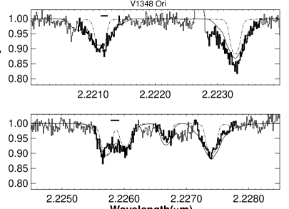
Figure 3: K-band infrared spectra of V1348 Ori are shown in the histogram. The spectral regions shown in bold are the magnetically sensitive Ti I lines actually used in the fit. The dash-dotted lines show a model with no magnetic field. The smooth lines are the best fit with magnetic broadening based on model 3. The solid horizontal bars mark the wavelengths where telluric absorption is stronger than 3% of the continuum and coincides with the lines used in the fit. The emission feature at 2.2227 $\mu$m is a molecular hydrogen line.

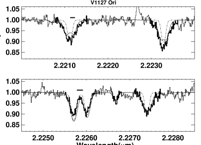
Figure 7: K-band infrared spectra of V1227 Ori are shown in the histogram. The spectral regions shown in bold are the magnetically sensitive Ti I lines actually used in the fit. The dash-dotted lines show a model with no magnetic field. The smooth lines are the best fit with magnetic broadening based on model 3. The solid horizontal bars mark the wavelengths where telluric absorption is stronger than 3% of the continuum and coincides with the lines used in the fit.

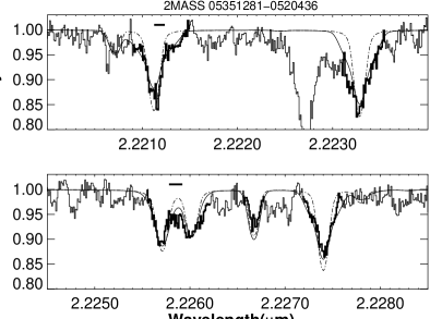
Figure 8: K-band infrared spectra of 2MASS 05351281-0520436.

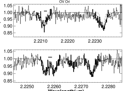
Figure 9: K-band infrared spectra of OV Ori.

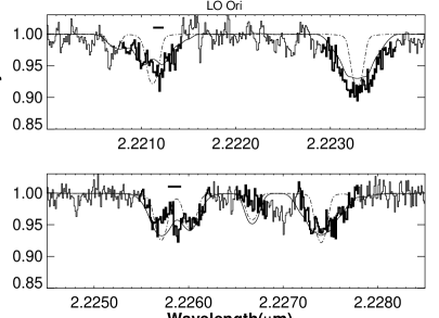
Figure 10: K-band infrared spectra of LO Ori.

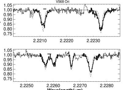
Figure 11: K-band infrared spectra of V568 Ori.

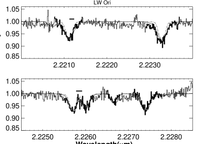
Figure 12: K-band infrared spectra of LW Ori.

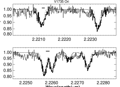
Figure 13: K-band infrared spectra of V1735 Ori.

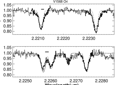
Figure 14: K-band infrared spectra of V1568 Ori.

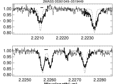
Figure 15: K-band infrared spectra of 2MASS 05361049-0519449.

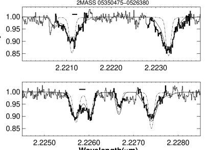
Figure 16: K-band infrared spectra of 2MASS 05350475-0526380.

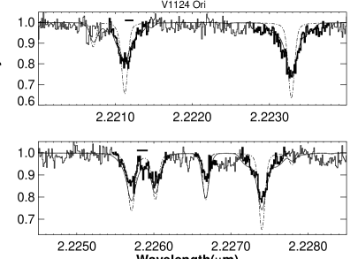
Figure 17: K-band infrared spectra of V1124 Ori.

As examples of the fits, the K-band spectra of 2MASS 05353126-0518559, V1123 Ori, and V1348 Ori are shown in Figures 1–3. (The spectra of other targets are presented as online-only Figures 7-17.) When correcting the observed spectra for telluric absorption, there are only two particularly strong telluric lines that affect the photospheric lines used in our analysis. The horizontal bars in Figures 1–3 mark the two telluric features that are stronger than 3% of the continuum. Though these two regions are likely to have higher uncertainties than the regions that not affected by telluric absortion, Johns-Krull et al. (2009) found that arbitrarily increasing the uncertainties of the pixels in Phoenix data that are significantly affected by the telluric correction has essentially no effect on the fitting results. The Phoenix data used here is even less affected by telluric contamination and we expect uncertainties in its correction to have similarly negligible effect. To show an example of how sensitive our analysis is to the uncertainties in $T_{\rm eff}$, we analyze 2MASS 05353126-0518559 with a $T_{\rm eff}$ that is $\pm\ 300$ K from the value we used (3900 K), and the measured magnetic field values are changed by only 3% ($-300$ K) and 8% ($+300$ K). As demonstrated in Paper III, small errors in $T_{\rm eff}$ and $\log g$ in general only affect the magnetic field measurements by a few percent.

Additional errors might be incurred by errors in $v\sin i$ values, as we do not have magnetically insensitive CO lines to check on the atmospheric parameters (in particular $v\sin i$) used in the spectrum synthesis. However, the lack of CO line data is not expected to be a major issue for this work. In previous papers in this series, the CO data have largely served as a check on optically determined $v\sin i$ measurements. For example, Johns-Krull (2007) did use $v\sin i$ measurements determined from the CO data for most stars in that study. These $v\sin i$ values were published in Johns-Krull & Valenti (2001) where it was shown that the CO determined $v\sin i$ values are consistent with optically determined values such as those used in the present study. To estimate the effect of uncertainties in $v\sin i$ on the recovered values of $\bar{B}$, we have repeated the analysis of 2MASS 05353126-0518559 (medium $v\sin i$, strong field) and V568 Ori (low $v\sin i$, weaker field) where we have held the vsini of each star fixed at values corresponding to $\pm 1$ km s^-1 (a typical uncertainty). In the case of the 2MASS star, the resulting change in $\bar{B}$ was 1% and 3%, and in the case of V568 Ori the resulting change was 1.5% and 8%. The reason for such a small effect of the recovered field is that the magnetic broadening is significantly stronger than the rotational broadening in the Ti I lines. To make a final estimate of our field uncertainties from possible inaccuracies in stellar parameters, we conservatively assume a 10% uncertainty resulting from mismatches in both $T_{\rm eff}$ and $\log g$  and add these together in quadrature with an 8% uncertainty resulting from errors in the adopted $v\sin i$. These sources of uncertainties add up to 16 %. For most of our stars, there is a noticeable decrease in $\chi^{2}$ for models 2 and 3 relative to the single-component model (1). The two stars for which this is not the case are OV Ori and LW Ori, which both have relatively low signal-to-noise spectra. On the other hand, models 2 and 3 do not agree perfectly, even though they do generally return mean fields that agree to within the 16% uncertainty described above. Therefore, we adopt as our final mean field value the average mean field returned by models 2 and 3. We take the difference between this mean and the individual values as an estimate of the uncertainty of the technique, and add it in quadrature to the 16% uncertainty described above. For OV Ori and LW Ori, we average the mean field from all 3 models and take the standard deviation as the an estimate of the uncertainty, which is added in quadrature to the 16% uncertainty. The final $\bar{B}$ values and the associated uncertainties are listed in the last two columns of Table 3. We use the adopted values of $\bar{B}$ and its uncertainty, and propagate them through all subsequent calculations and comparisons.

Table 3: Magnetic-Field Measurements.

Object	Type		Model 1			Model 2			Model 3			Adopted
		$\chi_{r}^{2}$ (B=0)	$\bar{B}$ (kG) ($\chi_{r}^{2}$)	$r_{K}$		$\bar{B}$ (kG) ($\chi_{r}^{2}$)	$r_{K}$		$\bar{B}$ (kG) ($\chi_{r}^{2}$)	$r_{K}$		$\bar{B}$ (kG)	$\sigma$ (kG)
2MASS 05353126-0518559	CTTS	14.19	1.91 (1.99)	0.85		2.68 (1.60)	1.03		2.99 (1.62)	1.05		2.84	0.48
V1227 Ori	CTTS	11.99	1.81 (3.00)	0.72		2.13 (2.50)	0.62		2.15 (2.77)	0.65		2.14	0.34
2MASS 05351281-0520436	CTTS	17.85	1.41 (1.85)	0.63		1.81 (1.81)	0.81		1.58 (1.82)	0.66		1.70	0.29
V1123 Ori	NTTS	9.71	1.94 (3.09)	0.00		2.43 (2.64)	0.00		2.58 (2.69)	0.00		2.51	0.41
OV Ori	CTTS	3.16	1.55 (1.10)	0.59		1.64 (1.19)	0.63		2.35 (1.06)	0.72		1.85	0.53
V1348 Ori	CTTS	9.78	2.05 (3.54)	0.38		3.05 (3.14)	0.52		3.23 (2.74)	0.58		3.14	0.51
LO Ori	CTTS	9.45	2.70 (2.81)	1.44		3.26 (2.52)	1.61		3.63 (2.41)	1.56		3.45	0.58
V568 Ori	CTTS	10.98	1.32 (1.83)	0.64		1.59 (1.30)	0.65		1.46 (1.39)	0.55		1.53	0.25
LW Ori	CTTS	8.30	1.04 (1.32)	1.43		1.32 (1.33)	1.56		1.55 (1.30)	1.58		1.30	0.33
V1735 Ori	NTTS	3.12	1.54 (1.47)	0.00		2.14 (1.38)	0.00		2.01 (1.38)	0.00		2.08	0.34
V1568 Ori	NTTS	4.00	1.06 (2.16)	0.00		1.42 (1.77)	0.00		1.42 (2.01)	0.00		1.42	0.23
2MASS 05361049-0519449	CTTS	9.99	1.66 (2.10)	0.24		2.28 (1.71)	0.26		2.34 (1.67)	0.25		2.31	0.37
2MASS 05350475-0526380	CTTS	13.95	1.97 (2.90)	0.60		2.81 (2.42)	0.79		2.76 (2.44)	0.70		2.79	0.45
V1124 Ori	NTTS	8.90	1.45 (3.90)	0.00		2.17 (3.19)	0.00		2.00 (3.25)	0.00		2.09	0.34

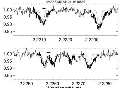
Figure 1: K-band infrared spectra of 2MASS 05353126-0518559 are shown in the histogram. The spectral regions shown in bold are the magnetically sensitive Ti I lines actually used in the fit. The dash-dotted lines show a model with no magnetic field. The smooth lines are the best fit with magnetic broadening based on model 3. The solid horizontal bars mark the wavelengths where telluric absorption is stronger than 3% of the continuum and coincides with the lines used in the fit.

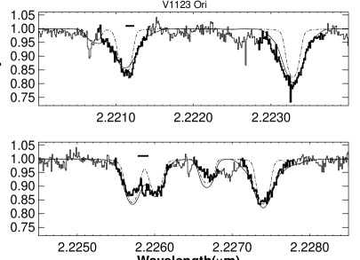
Figure 2: K-band infrared spectra of V1123 Ori are shown in the histogram. The spectral regions shown in bold are the magnetically sensitive Ti I lines actually used in the fit. The magnetically sensitive Ti I lines are in bold. The dash-dotted lines show a model with no magnetic field. The smooth lines are the best fit with magnetic broadening based on model 3. The solid horizontal bars mark the wavelengths where telluric absorption is stronger than 3% of the continuum and coincides with the lines used in the fit.

4 DISCUSSION

For 14 T Tauri stars in the ONC, we model the Zeeman broadening in three magnetically sensitive Ti I lines and measure the mean surface magnetic field strengths on these stars. We have attempted to account for various sources of uncertainty in our measurements, but there are some potential sources for which this is quite difficult. An example of this is the assumed geometry of the field. We have assumed a purely radial field geometry in the spectrum synthesis. This was originally motivated by analogy to the Sun where observations suggested surface fields (at least in high flux density regions) are primarily oriented along the vertical direction (e.g., Stenflo, 2010). A number of recent Zeeman Doppler Imaging (ZDI) studies have begun to provide surface maps of magnetic fields on T Tauri stars (e.g., Donati et al., 2007, 2008, 2010; Hussain et al., 2009). These studies show that the field topology is not purely radial; however, it is not at all clear that the ZDI results give an accurate picture of the majority of the magnetic flux on the star. Reiners & Basri (2009) showed that in strongly magnetic M stars, Stokes V based studies (ZDI) miss 86% or more of the magnetic flux present compared to Stokes I based studies due to the effects of flux cancellation in Stokes V measurements which are not present in Stokes I measurements.

Our work here is based on Stokes I. If the field were entirely aimed along the line of sight, or entirely perpendicular to it, the relative strength of the $\pi$ and $\sigma$ Zeeman components would change and affect our results somewhat. However, the polarization measurements mentioned above show such pathological field orientations are generally not present (see also Johns-Krull et al., 1999a; Daou et al., 2006; Yang et al., 2007). Instead, there is likely a stong mixture of field orientations on the star: some parallel to the line of sight, some perpendicular to the line of sight, and all angles in between. While we assume a radial geometry on the star, when we integrate over the visible stellar disk, we then include a good mixture of field lines with all orientations to the line of sight. As a result, we do not expect our results to be strongly affected by our assumption of a radial field geometry. Again, as mentioned above, since the ZDI results likely do not provide good guidance for the geometry of the total field (Reiners & Basri, 2009), this is probably the best we can do until better guidance comes from theory or even better observations.

For most of our targets, the single magnetic component fit of model 1 is not good enough to account for all the excess broadening in the observed line profiles. For a few targets such as OV Ori and LW Ori, adding more magnetic components does not improve the fits significantly. That is due to a combination of low signal-to-noise ratios and small magnetic broadening. Models 2 and 3 generally yield higher mean magnetic field strengths and better matches to the observations, resulting in lower reduced $\chi^{2}$ values. In most cases, the mean field values recovered by models 2 and 3 are in good agreement with similar reduced $\chi^{2}$ values. On average, the difference between the two recovered values is less than 9%.

Since we apply models that are consistent with previous studies of 14 stars in Taurus (Johns-Krull, 2007) and 5 stars in the TW Hydrae association (Papers III and IV), we are able to directly compare the measurements of all 33 stars in the three regions. Out of the 33 stars in total, 27 stars have spectral types between K7 and M3. The rest of the sample have spectral types between K3 and K6, except for the K0 star T Tau. Therefore, these stars possess similar spectral properties and allow a meaningful comparison. We calculate stellar ages using the pre-MS evolutionary tracks of Siess et al. (2000), and plot the measured magnetic field values and magnetic fluxes ($4\pi{R_{*}}^{2}\bar{B}$) against stellar ages, shown in Figures 4 and 5, respectively. We note that while stellar magnetic field strength spans a range of values and displays no apparent correlation with stellar age, stellar magnetic flux decreases consistently with time. The primary reason for the inverse correlation of magnetic flux with age is the diminishing stellar radii as the stars evolve down their Hyashi tracks. However, as shown below, the measured fields/fluxes do not correlate with any other expected dynamo properties, including for example the stellar gravity. As a result, we find no evidence the the field strengths are being set by some other property of the stars, which might produce an inverse correlation with age/radius as a by-product. The observed trend of the flux decreasing with age supports the idea that the strong magnetic fields of TTSs could be of primordial origin. As suggested by Moss (2003), during the early stages of stellar evolution, while primordial magnetic flux does decay, young stars may be able to maintain part of the fossil flux from the molecular cloud material, especially later when a raditive core is formed. It should be noticed that currently there are only a few measurements for stars younger than 1 Myr or older than 10 Myr, so more observations are needed to further trace out the evolution of stellar magnetic fields with time.

Figure 4: Measured magnetic fields plotted against age for the Orion, Taurus/Auriga and TWA Stars. The triangles represent the Orion stars from this work. The filled circles represent the TWA stars from Papers III and IV, and the hollow diamonds are the Taurus/Auriga stars from Johns-Krull (2007). The sizes of error bars are 10% for the TWA and Taurus/Auriga stars and the values in the last column of Table 3 for the Orion stars.

Figure 5: Measured magnetic flux plotted against age for the Orion, Taurus/Auriga and TWA Stars. The triangles represent the Orion stars from this work. The filled circles represent the TWA stars from Papers III and IV, and the hollow diamonds are the Taurus/Auriga stars from Johns-Krull (2007).

In addition to a fossil origin for the magnetic fields on young stars, these observed strong fields could in principle be the result of dynamo action, either a solar-like $\alpha-\Omega$ dynamo (Durney & Latour, 1978; Parker, 1993) or as a result of a distributed, turbulent or convective dynamo (e.g., Durney et al., 1993). In current $\alpha-\Omega$ dynamo models, magnetic fields are generated by differential rotation at the region between the radiative interior and the outer convective shell, a region known as the tachocline. In such a dynamo, it is believed that levels of magnetic activity are related to the Rossby number, defined as $P_{rot}/\tau_{c}$, where $P_{rot}$ is the rotation period and $\tau_{c}$ is the convective turnover time. However, Johns-Krull (2007) found no correlation for 14 Taurus stars and TW Hya between the measured magnetic field values and various stellar or dynamo parameters. Here, for a combined sample of 31 stars from Yang et al. (2008), Johns-Krull (2007) and this study, we look for a correlation between measured magnetic properties and various potential dynamo parameters. We obtain $\tau_{c}$ from models described in Kim & Demarque (1996) and Preibisch et al. (2005). In Table 4, we give the Pearson linear correlation coefficient, $r$, and its false alarm probability, $f_{p}$, for several comparisons. No significant correlation is seen between the observed magnetic field strength/flux and any dynamo parameter. Such lack of correlation is generally contrary to the prediction of theories of solar-like interface dynamos. Besides interface dynamos, there are models that involve a distributed dynamo (e.g., Durney et al., 1993). This kind of dynamo is thought to be able to operate in fully convective stars such as TTSs and create large-scale magnetic fields via convective motions. Recently, Christensen et al. (2009) extended a scaling law derived from convection-driven geodynamo models to the regime of stars, including TTSs, and their predictions for the field strengths on TTSs are generally consistent with the observed values. However, magnetic fields generated by a distributed dynamo are also expected to have a dependence, though possibly weak, on rotation(Durney et al., 1993; Chabrier & Küker, 2006), which we do not observe. Therefore, we suggest that the survival of the fossil magnetic flux seems to be a more promising explanation for the origin of strong magnetic fields on TTSs; however, more work in this area is needed.

Table 4: Correlations of Measured Magnetic Parameters with Dynamo Parameters

Quantities Compared	$r$	$f_{p}$
$\bar{B}$ vs. $P_{rot}^{-1}$	-0.01	0.94
$\Phi$ vs. $P_{rot}^{-1}$	-0.04	0.83
$\bar{B}$ vs. $\tau_{c}$	0.24	0.20
$\Phi$ vs. $\tau_{c}$	-0.08	0.64
$\bar{B}$ vs. $\tau_{c}P_{rot}^{-1}$	0.05	0.79
$\Phi$ vs. $\tau_{c}P_{rot}^{-1}$	-0.15	0.42
$\bar{B}$ vs. $\log g$	0.14	0.46
$\Phi$ vs. $\log g$	-0.45	0.01

We also examine the relationship between magnetic flux and the X-ray properties of the ONC stars. As first noted by Pevtsov et al. (2003) for the Sun and a number of main-sequence dwarfs, there is a nearly linear correlation between X-ray luminosities, $L_{\rm x}$, and the total unsigned magnetic flux, $\Phi$. The correlation holds over 12 orders of magnitude in both quantities. We use this relationship with our measured magnetic flux values to calculate the predicted X-ray luminosities for our ONC stars. These values are listed in Table 5, where we compare them with the observed values reported by Flaccomio et al. (2003) and Getman et al. (2005). The typical uncertainty in the observed $L_{x}$ is 0.2 dex. The comparison is also plotted in Figure 6. On average, the predicted $L_{x}$ values of the ONC stars are larger than the observed ones by a factor of $4.9\pm 1.4$. This suppression of the X-ray emission is consistently found as well for the Taurus and TWA stars, also shown in Figure 6, though the reduction is different in each region.

Large flares are thought to be responsible for harder X-ray emission on TTSs, while softer, persistent X-ray emission may be generated by so-called microflares that release energy from stressed magnetic fields in the coronae of these stars (Güdel et al., 2003; Arzner et al., 2007). On the Sun, these stresses are believed to be built up by convective motions acting on the footpoints of coronal loops. For TTSs, strong surface magnetic fields may decrease the efficiency by which convective gas motions are able to move footpoints around and build up these magnetic stresses. Thus, in addition to listing the measured magnetic field strengths based on model 3, $\bar{B}$, we also list in Table 5 the equipartition field strength, $B_{eq}={(8\pi P_{g})}^{1/2}$. This quantity is calculated assuming that the magnetic pressure, ${B_{eq}}^{2}/(8\pi)$, is in balance with the surrounding unmagnetized photospheric gas pressure, $P_{g}$. We use the gas pressure from a location in the model atmospheres where the local gas temperature is approximately equal to the effective temperature of the star. This level in the stellar photosphere is in the vinicity of where the observed continuum forms, so the gas pressure here should be generally greater than the regions where the Ti I lines form, setting an upper limit. The ratio of the observed field strength to the equipartition field strength ranges from 1.3 to 3.9 for the ONC stars, indicating the dominance of magnetic pressure over gas pressure in the photospheres of these TTSs. This dominance of magnetic pressure may partially prohibit the production of X-ray emission. Since these ratios of the ONC stars are close to those of the TWA stars, it is likely no coincidence that in Figure 6 the observed X-ray luminosities of most ONC stars are smaller than the predicted values by a similar factor as those of the TWA stars.

Table 5: Magnetic-Field Properties and X-Ray Luminosities.

Object	$\bar{B}$	$B_{eq}$	Predicted $\log L_{X}$	Observed $\log L_{X}$
	(kG)	(kG)	(erg/s)	(erg/s)
2MASS 05353126-0518559	2.84	0.99	31.16	30.37
V1227 Ori	2.14	0.87	30.49	30.20
2MASS 05351281-0520436	1.70	1.03	30.65	29.65
V1123 Ori	2.51	1.00	30.98	30.65
OV Ori	1.85	1.07	30.73	N/A
V1348 Ori	3.14	1.00	30.86	30.63
LO Ori	3.45	0.99	30.75	$<$30.23
V568 Ori	1.53	1.07	30.47	30.04
LW Ori	1.30	1.00	30.37	29.63
V1735 Ori	2.08	1.35	N/A	N/A
V1568 Ori	1.42	0.93	30.61	$<$30.38
2MASS 05361049-0519449	2.31	1.42	30.85	30.69
2MASS 05350475-0526380	2.79	1.02	30.81	30.45
V1124 Ori	2.09	1.67	30.70	30.29

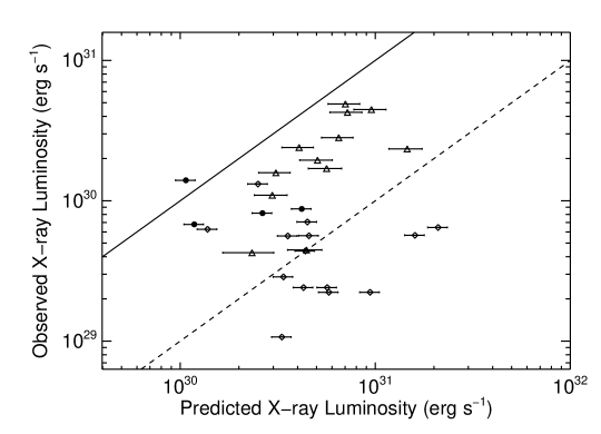
Figure 6: Observed X-ray luminosity plotted against the predicted X-ray luminosity for the Orion, Taurus/Auriga and TWA stars. The solid line is the line of equality, and the dashed line is where the predicted value is 10 times the observed one. The triangles represent the Orion stars from this work. The filled circles represent the TWA stars from Paper IV, and the hollow diamonds are the Taurus/Auriga stars from Johns-Krull (2007).

5 Conclusion

By modeling the Zeeman broadening in three magnetically sensitive Ti I lines, we consistently measure kilogauss-level magnetic fields in the photospheres of 14 TTSs in the ONC. We find a systematic decrease of stellar magnetic flux from the young Orion region ($\sim$ 1 Myr), through the Taurus region ($\sim$ 2 Myr), to the TWA ($\sim$ 10 Mys). This finding supports a primordial origin of the magnetic fields on TTSs, though recent convective dynamos by Christensen et al. (2009) are able to produce magnetic fields that have strengths consistent with observations. Because convective motions are likely partially inhibited by the dominance of magnetic pressure over unmagnetized gas pressure in the stellar photospheres, the strong magnetic fields could also be responsible for suppression of X-ray emission on TTSs relative to that expected from main sequence star calibrations.

Appendix A Online-Only Figures

References

- Allard & Hauschildt (1995) Allard, F., & Hauschildt, P. H. 1995, ApJ, 445, 433
- Arzner et al. (2007) Arzner, K., Güdel, M., Briggs, K., Telleschi, A., & Audard, M. 2007, A&A, 468, 477
- Bally et al. (2000) Bally, J., O’Dell, C. R., & McCaughrean, M. J. 2000, AJ, 119, 2919
- Barrado Y Navascués (2006) Barrado Y Navascués, D. 2006, A&A, 459, 511
- Bevington & Robinson (1992) Bevington, P. R., & Robinson, D. K. 1992, Data reduction and error analysis for the physical sciences (2nd ed.; New York: McGraw-Hill)
- Bouvier et al. (2007) Bouvier, J., Alencar, S. H. P., Harries, T. J., Johns-Krull, C. M., & Romanova, M. M. 2007, in Protostars and Planets V, ed. B. Reipurth, D. Jewitt, & K. Keil (Tucson, AZ: Univ. of Arizona Press), 479
- Camenzind (1990) Camenzind, M. 1990, in Reviews in Modern Astronomy, ed. G. Klare (Berlin: Springer), 234
- Carpenter et al. (2001) Carpenter, J. M., Hillenbrand, L. A., & Skrutskie, M. F. 2001, AJ, 121, 3160
- Chabrier & Küker (2006) Chabrier, G., & Küker, M. 2006, A&A, 446, 1027
- Christensen et al. (2009) Christensen, U. R., Holzwarth, V., & Reiners, A. 2009, Nature, 457, 167
- Collier Cameron & Campbell (1993) Collier Cameron, A., & Campbell, C. G. 1993, A&A, 274, 309
- Daou et al. (2006) Daou, A. G., Johns-Krull, C. M., & Valenti, J. A. 2006, AJ, 131, 520
- Donati et al. (2007) Donati, J., Jardine, M. M., Gregory, S. G., Petit, P., Bouvier, J., Dougados, C., Ménard, F., Cameron, A. C., Harries, T. J., Jeffers, S. V., & Paletou, F. 2007, MNRAS, 380, 1297
- Donati et al. (2010) Donati, J., Skelly, M. B., Bouvier, J., Jardine, M. M., Gregory, S. G., Morin, J., Hussain, G. A. J., Dougados, C., Ménard, F., & Unruh, Y. 2010, MNRAS, 402, 1426
- Donati et al. (2008) Donati, J.-F., Jardine, M. M., Gregory, S. G., Petit, P., Paletou, F., Bouvier, J., Dougados, C., Ménard, F., Cameron, A. C., Harries, T. J., Hussain, G. A. J., Unruh, Y., Morin, J., Marsden, S. C., Manset, N., Aurière, M., Catala, C., & Alecian, E. 2008, MNRAS, 386, 1234
- Durney et al. (1993) Durney, B. R., De Young, D. S., & Roxburgh, I. W. 1993, Sol. Phys., 145, 207
- Durney & Latour (1978) Durney, B. R., & Latour, J. 1978, Geophys. Astrophys. Fluid Dyna., 9, 241
- Flaccomio et al. (2003) Flaccomio, E., Damiani, F., Micela, G., Sciortino, S., Harnden, Jr., F. R., Murray, S. S., & Wolk, S. J. 2003, ApJ, 582, 382
- Getman et al. (2005) Getman, K. V., Flaccomio, E., Broos, P. S., Grosso, N., Tsujimoto, M., Townsley, L., Garmire, G. P., Kastner, J., Li, J., Harnden, Jr., F. R., Wolk, S., Murray, S. S., Lada, C. J., Muench, A. A., McCaughrean, M. J., Meeus, G., Damiani, F., Micela, G., Sciortino, S., Bally, J., Hillenbrand, L. A., Herbst, W., Preibisch, T., & Feigelson, E. D. 2005, ApJS, 160, 319
- Greene et al. (1993) Greene, T. P., Tokunaga, A. T., Toomey, D. W., & Carr, J. B. 1993, in Proc. SPIE Vol. 1946, p. 313-324, Infrared Detectors and Instrumentation, Albert M. Fowler; Ed., ed. A. M. Fowler, 313–324
- Güdel et al. (2003) Güdel, M., Audard, M., Kashyap, V. L., Drake, J. J., & Guinan, E. F. 2003, ApJ, 582, 423
- Hillenbrand (1997) Hillenbrand, L. A. 1997, AJ, 113, 1733
- Hinkle et al. (2003) Hinkle, K. H., Blum, R. D., Joyce, R. R., Sharp, N., Ridgway, S. T., Bouchet, P., van der Bliek, N. S., Najita, J., & Winge, C. 2003, in Proceedings of the Society of Photo-Optical Instrumentation Engineers (SPIE) Conference, Vol. 4834, Discoveries and Research Prospects from 6- to 10-Meter-Class Telescopes II., ed. P. Guhathakurta, 353
- Hirota et al. (2007) Hirota, T., Bushimata, T., Choi, Y. K., Honma, M., Imai, H., Iwadate, K., Jike, T., Kameno, S., Kameya, O., Kamohara, R., Kan-Ya, Y., Kawaguchi, N., Kijima, M., Kim, M. K., Kobayashi, H., Kuji, S., Kurayama, T., Manabe, S., Maruyama, K., Matsui, M., Matsumoto, N., & Miyaji, T. 2007, PASJ, 59, 897
- Hussain et al. (2009) Hussain, G. A. J., Collier Cameron, A., Jardine, M. M., Dunstone, N., Ramirez Velez, J., Stempels, H. C., Donati, J., Semel, M., Aulanier, G., Harries, T., Bouvier, J., Dougados, C., Ferreira, J., Carter, B. D., & Lawson, W. A. 2009, MNRAS, 398, 189
- Jeffries (2007) Jeffries, R. D. 2007, MNRAS, 381, 1169
- Johns-Krull (2007) Johns-Krull, C. M. 2007, ApJ, 664, 975
- Johns-Krull et al. (2009) Johns-Krull, C. M., Greene, T. P., Doppmann, G. W., & Covey, K. R. 2009, ApJ, 700, 1440
- Johns-Krull & Valenti (1996) Johns-Krull, C. M., & Valenti, J. A. 1996, ApJ, 459, L95
- Johns-Krull & Valenti (2001) —. 2001, ApJ, 561, 1060
- Johns-Krull et al. (1999a) Johns-Krull, C. M., Valenti, J. A., Hatzes, A. P., & Kanaan, A. 1999a, ApJ, 510, L41
- Johns-Krull et al. (1999b) Johns-Krull, C. M., Valenti, J. A., & Koresko, C. 1999b, ApJ, 516, 900
- Johns-Krull et al. (2004) Johns-Krull, C. M., Valenti, J. A., & Saar, S. H. 2004, ApJ, 617, 1204
- Johnson (1966) Johnson, H. L. 1966, ARA&A, 4, 193
- Kim & Demarque (1996) Kim, Y.-C., & Demarque, P. 1996, ApJ, 457, 340
- Königl (1991) Königl, A. 1991, ApJ, 370, L39
- Ménard & Bertout (1999) Ménard, F., & Bertout, C. 1999, in The Origin of Stars and Planetary Systems, ed. C. J. Lada & N. D. Kylafis (NATO ASIC Proc. 540; Dordrecht: Kluwer), 341
- Moss (2003) Moss, D. 2003, A&A, 403, 693
- O’dell (2001) O’dell, C. R. 2001, ARA&A, 39, 99
- Paatz & Camenzind (1996) Paatz, G., & Camenzind, M. 1996, A&A, 308, 77
- Palla & Stahler (2000) Palla, F., & Stahler, S. W. 2000, ApJ, 540, 255
- Parker (1993) Parker, E. N. 1993, ApJ, 408, 707
- Petrov (2003) Petrov, P. P. 2003, Astrophysics, 46, 506
- Pevtsov et al. (2003) Pevtsov, A. A., Fisher, G. H., Acton, L. W., Longcope, D. W., Johns-Krull, C. M., Kankelborg, C. C., & Metcalf, T. R. 2003, ApJ, 598, 1387
- Piskunov (1999) Piskunov, N. 1999, in Astrophysics and Space Science Library, Vol. 243, Polarization, ed. K. N. Nagendra & J. O. Stenflo (Dordrecht: Kluwer), 515
- Preibisch et al. (2005) Preibisch, T., Kim, Y.-C., Favata, F., Feigelson, E. D., Flaccomio, E., Getman, K., Micela, G., Sciortino, S., Stassun, K., Stelzer, B., & Zinnecker, H. 2005, ApJS, 160, 401
- Reiners & Basri (2009) Reiners, A., & Basri, G. 2009, A&A, 496, 787
- Robinson (1980) Robinson, Jr., R. D. 1980, ApJ, 239, 961
- Saar (1988) Saar, S. H. 1988, ApJ, 324, 441
- Sandstrom et al. (2007) Sandstrom, K. M., Peek, J. E. G., Bower, G. C., Bolatto, A. D., & Plambeck, R. L. 2007, ApJ, 667, 1161
- Shu et al. (1994) Shu, F., Najita, J., Ostriker, E., Wilkin, F., Ruden, S., & Lizano, S. 1994, ApJ, 429, 781
- Sicilia-Aguilar et al. (2005) Sicilia-Aguilar, A., Hartmann, L. W., Szentgyorgyi, A. H., Fabricant, D. G., Fűrész, G., Roll, J., Conroy, M. A., Calvet, N., Tokarz, S., & Hernández, J. 2005, AJ, 129, 363
- Siess et al. (2000) Siess, L., Dufour, E., & Forestini, M. 2000, A&A, 358, 593
- Stenflo (2010) Stenflo, J. O. 2010, A&A, 517, A37+
- Tayler (1987) Tayler, R. J. 1987, MNRAS, 227, 553
- Tokunaga et al. (1990) Tokunaga, A. T., Toomey, D. W., Carr, J., Hall, D. N. B., & Epps, H. W. 1990, in Instrumentation in astronomy VII; Proceedings of the Meeting, Tucson, AZ, Feb. 13-17, 1990 (A91-29601 11-35). Bellingham, WA, Society of Photo-Optical Instrumentation Engineers, 1990, p. 131-143., ed. D. L. Crawford, 131–143
- Valenti et al. (1995) Valenti, J. A., Marcy, G. W., & Basri, G. 1995, ApJ, 439, 939
- Yang et al. (2005) Yang, H., Johns-Krull, C. M., & Valenti, J. A. 2005, ApJ, 635, 466
- Yang et al. (2007) —. 2007, AJ, 133, 73
- Yang et al. (2008) —. 2008, AJ, 136, 2286