Variability and Multiwavelength Detected AGN in the GOODS Fields

Abstract

We identify 85 variable galaxies in the GOODS North and South fields using 5 epochs of HST ACS V-band (F606W) images spanning 6 months. The variables are identified through significant flux changes in the galaxy’s nucleus and represent $\sim$2% of the survey galaxies. With the aim of studying the active galaxy population in the GOODS fields, we compare the variability-selected sample with X-ray and mid-IR AGN candidates. Forty-nine percent of the variables are associated with X-ray sources identified in the 2Ms Chandra surveys. Twenty-four percent of X-ray sources likely to be AGN are optical variables and this percentage increases with decreasing hardness ratio of the X-ray emission. Stacking of the non-X-ray detected variables reveals marginally significant soft X-ray emission. Forty-eight percent of mid-IR power-law sources are optical variables, all but one of which are also X-ray detected. Thus, about half of the optical variables are associated with either X-ray or mid-IR power-law emission. The slope of the power-law fit through the Spitzer IRAC bands indicates that two-thirds of the variables have BLAGN-like SEDs. Among those galaxies spectroscopically identified as AGN, we observe variability in 74% of broad-line AGNs and 15% of NLAGNs. The variables are found in galaxies extending to z$\sim$3.6. We compare the variable galaxy colors and magnitudes to the X-ray and mid-IR sample and find that the non-X-ray detected variable hosts extend to bluer colors and fainter intrinsic magnitudes. The variable AGN candidates have Eddington ratios similar to those of X-ray selected AGN.

1 INTRODUCTION

Active Galactic Nuclei (AGNs) are galaxies accreting significant amounts of material onto their central supermassive black holes (SMBHs). These galaxies were once thought to be oddities among the total galaxy population, but are now seen as important mile markers on the broad road of galaxy evolution. Once considered rare, SMBHs are now believed to exist in the centers of all galaxies containing a significant bulge component (Kormendy & Richstone 1995). In addition, the observed relation between the mass of the SMBH and the bulge stellar mass (Ferrarese & Merritt 2000; Gebhardt et al. 2000) suggests a coupled assembly history between the two. To understand the role played by AGN in the evolution of galaxies, it is thus necessary to identify complete samples of AGN in galaxy surveys.

AGN have been identified using many techniques such as UV/optical color selection (Markarian 1967; Schmidt & Green 1983; Richards et al. 2002), spectroscopic signatures of broad emission lines or narrow emission lines with distinct line flux ratios (Baldwin et al. 1981; Veilleux & Osterbrock 1987), X-ray emission (Fabbiano et al. 1992; Alexander et al. 2003), infrared color selection (Lacy et al. 2004; Stern et al. 2005), radio emission (e.g. Smith & Wright 1980) and variability (e.g. Hook et al. 1994; MacLeod et al. 2010) over a range of timescales. Many of these techniques, however, produce samples biased against galaxies where the AGN light is much less than that of the host galaxy. Additionally, most surveys in the optical/UV are biassed against obscured, dusty AGN/host galaxies. In order to identify largely complete samples of AGN, it is clear that a variety of techniques and selection methods should be employed. While it may be found that AGN selected using different techniques represent separate populations experiencing different phases in AGN/galaxy evolution (e.g. Hickox et al. 2009), a less biased sample of AGN will help to make this picture clearer and allow us to better interpret the role AGN play within their host galaxies.

In this paper, we aim to identify AGN in the Great Observatories Origins Deep Survey (GOODS) North and South fields beginning with an optical variability selected sample. AGN are known to vary on timescales of months to years in the optical with 90–100% of AGN identified via other means observed to vary over the course of several years (e.g. Koo et al. 1986; Schmidt et al. 2010). The mechanism behind the variability is still uncertain, though the leading explanation involves disk instabilities (Pereyra et al. 2006) or changes in the amount of infalling material (Hopkins et al. 2006). Regardless of the physics behind variability, AGN are observed to display brightness variations of several percent over many years. There is additional evidence of an increase in variability amplitude for intrinsically fainter AGN (Bershady et al. 1998; Vanden Berk et al. 2004) making variability a particularly effective means for identifying low-luminosity AGN. We build on the results of previous successful surveys to identify AGN candidates in the nuclei of galaxies found in deep HST surveys (e.g. Sarajedini et al. 2003). The high resolution HST images allow us to obtain accurate photometry within small apertures (r$\mathrel{\hbox{\hbox to0.0pt{\hbox{\lower 4.0pt\hbox{$\sim$}}\hss}\hbox{$<$}}}$0.2${}^{\prime\prime\,}$), thus allowing us to probe lower AGN/host galaxy luminosity ratios than can be done using ground-based images. We expect $\sim$60% of AGN in the GOODS fields to be identified as variable with the time sampling of 5 epochs separated by 45-day intervals. This estimate is based on the results of Webb & Malkan (2000), who found that 60% of Seyfert/QSOs in their study revealed significant variability on month-to-month timescales.

We also explore X-ray and mid-IR selected AGN identified in the GOODS fields and compare with the variability survey. These wavelengths are powerful probes of AGN and are especially important for uncovering obscured sources. The multiwavelength data provide important confirmations of the AGN nature of the variables as well as the quantification of the use of optical variability in identifying sources of varying levels of obscuration. We also compare the variables to spectroscopically selected AGN in the GOODS fields.

We describe the AGN sample drawn from the variability analysis in §2. In §3 we compare this sample to those identified via X-rays, mid-IR power-law SEDs, and optical spectroscopy. We discuss the redshift distribution, absolute magnitudes, and colors of the variables, X-ray and mid-IR AGN in §4. In §5 we discuss how variability selected AGN fit with the current picture of AGN/galaxy evolution in part by deriving Eddington ratios for the variables in our survey. Throughout the paper we assume a flat, cosmological constant-dominated cosmology with parameter values $\Omega$_Λ = 0.7, $\Omega$_M = 0.3, and H_o = 70 km/s/Mpc. The data presented in this paper are in the AB photometric system.

2 DATA ANALYSIS AND SELECTION OF VARIABLES

The GOODS fields consist of two regions of the sky, each $\sim$130 arcmin² in size and located at RA = 3h32m, Dec = -27d48m and RA = 12h37m, Dec = +62d15m. These fields were imaged with HST’s Advance Camera for Surveys Wide Field Camera (ACS WFC) in four passbands (F435W, F606W, F775W, and F850LP). All but the B-band images (F435W) were obtained in epochs separated by 45 days. We chose to perform our analysis using the F606W (hereafter, V-band) images to maximize sensitivity to varying AGN within host galaxies, given the fact that several studies find increased variability amplitude with decreasing wavelength (di Clemente et al. 1996; Sarajedini et al. 2003). The South field images were obtained between August 1 2002 and February 5 2003 with 5 epochs separated by $\sim$45 days for a total time baseline of 6 months. The North field images were obtained between November 21 2002 and May 23 2003 with the same time sampling as in the south. Two exposures per pointing per epoch were combined to produce an image with a total exposure time of $\sim$1000s.

The GOODS v2.0 source catalog ${(archive.stsci.edu/pub/hlsp/goods/catalog\_r2)}$ provided initial coordinate positions for identifying objects in the individual epoch ACS images. We found 11519 sources in the combined fields that were visible in all 5 epochs. To ensure that the centers of all sources were accurately determined and matched across the epochs, objects were recentered using the IRAF task ${\it center}$ and sources whose centers had large pixel shifts (i.e. more than 3$\sigma$ of the average shift for sources in a given ACS image) were visually inspected. Sources that fell too close to the CCD edge or with a cosmic ray close to the object center in one or more epochs were rejected. After this process, 10161 sources remained.

We used IRAF ${\it phot}$ to determine aperture photometry for each source using 3 aperture sizes, r$=$2.5 pixels, 3.5 pixels, and 5 pixels where the pixel scale is 0.05 arcsec/pix. The smallest aperture size is $\sim$twice the FWHM of a typical unresolved source and was initially selected as the primary aperture to identify AGN in galaxies, which should originate from an unresolved nuclear region. However, we carry out the variability analysis using the 5 pixel aperture data to ensure that changes in the PSF, which would be more significant for smaller apertures, do not result in an overestimate of variables. Magnitude differences were determined between epochs 2 through 5 and the first epoch. Small zeropoint offsets of 0.01 to 0.03 magnitude were determined among the epochs and applied to the photometry. For every source, we then determined the mean magnitude and standard deviation around the mean. We also calculate the concentration index, CI, as the magnitude difference between the r$=$2.5 pixel photometry and the r$=$5 pixel photometry. Point-like, unresolved sources should have small CI values while extended sources will occupy a range of higher values.

Figure 1 shows the mean nuclear V-band magnitude versus standard deviation for r$=$2.5 pixel apertures (Fig 1a), r$=$5 pixel apertures (Fig 1b), and the concentration index (Fig 1c). The expected increase in standard deviation values at fainter magnitudes is observed due to increasing photometric noise. The spread in standard deviation values is generally the same using either the small or large aperture photometry and would suggest that variations in the PSF are not producing significantly increased standard deviation scatter. Figure 1c shows a clear separation between the resolved and unresolved sources. Based on this figure, we define objects having CI values of $\leq$0.2 as unresolved or point-like and those with higher values as resolved or extended.

Applying this division, we find that unresolved sources generally have higher standard deviation values than do the extended sources across the range of magnitudes (Figure 2). The scatter in the standard deviation values do not decrease significantly when using the r$=$5 pixel photometry. We analyzed the unresolved sources using r$=$10 pixel aperture photometry as well and found a similar level of scatter. This higher level of scatter among the standard deviation values of the unresolved population is likely reflecting the difficulty in achieving photometric repeatability for point-like sources and may be enhanced by variations in the PSF which are not as significant for extended sources. Since simply using larger apertures does not reduce the scatter, we account for this difference by continuing the variability analysis separately for the unresolved and extended sources throughout the remainder of this paper. In this way, we determine the variability threshold for unresolved sources independently and can allow for this larger scatter. We use small apertures (r$=$2.5 pixel) for the extended sources to isolate the varying nuclei of galaxies and increase sensitivity. For the unresolved sources, we use the r$=$5 pixel apertures to avoid any possible sensitivity to PSF changes. In addition, since these are generally point-like in morphology, there is no need to use the smaller aperture to block light from an extended galaxy component.

We apply both a bright and faint magnitude cut to the variability survey. A bright limit of V${}_{2.5}=$20.0 was applied to remove several marginally saturated unresolved objects at the bright end of the distribution. These appear to be mainly foreground stars for which accurate photometry can not be determined. We identify the faint magnitude limit for our variability survey from the source number counts as a function of magnitude. The number of objects significantly drops beyond V${}_{2.5}=$26.5. Therefore, we limit the survey analysis to V${}_{2.5}=$26.0 to avoid significant photometric incompleteness.

To identify the variability threshold, the standard deviation values are separated into magnitude bins, allowing the bin limits to vary in size with larger bins at the bright end and smaller bins at the faint end to maintain similar numbers of objects ranging from 15 to 40 sources per bin. The greatest outliers from the mean magnitude of each bin were excluded and the resulting histograms were fit with Gaussians to determine the distribution center (mean standard deviation) and the sigma (i.e. spread) in standard deviation values at a given magnitude. At fainter magnitudes the standard deviation increases as well as the spread in those values. We fit a 2nd-order polynomial to both the mean standard deviation values in each bin and 1$\sigma$ of the Gaussian distribution in each bin. This is done in order to characterize the photometric error as a smoothly changing function of the source magnitude. Both the mean of the standard deviation and the spread in values around that mean are determined independently. Figures 3a and b show the variability plot for the GOODS South field with the mean standard deviation (solid thick line) and the mean plus 2-sigma and plus 3-sigma (dashed lines) for the point sources and extended sources separately. Figures 3c and 3d are the same for the North field. Determining the expected error at each magnitude in this empirical way provides the most realistic estimation of the photometric error on the standard deviation since we carry through the effects of object and sky Poisson noise, readout noise, and any limitations imposed by minor errors in the sky zero points used.

Sources at or above the mean standard deviation plus 3$\sigma$ were flagged for visual inspection. In the south field, 126 extended sources and 27 point sources were flagged and 94 extended and 10 point sources in the north field. Visual inspection of these outliers revealed that $\sim$50 in each field contained evidence of cosmic rays or fell in a location too close to the edge of a CCD and thus suffered from high background noise in one or more epochs. These sources were removed from the survey. About 15 objects per field were determined to have centering problems and these were manually recentered. With all outliers checked for accuracy, we recalculated the variability threshold for each field.

After comparing the variables against the known supernovae catalogs of Strolger et al. (2004), we identified one SN in the north and one in the south field from our extended source list. We also compare to several published redshift surveys (see §4) and identify a number of spectroscopically confirmed stars (11 in each of the fields). Since the aim of our paper to study the AGN population in these fields, we remove the known SNe and stars from the survey.

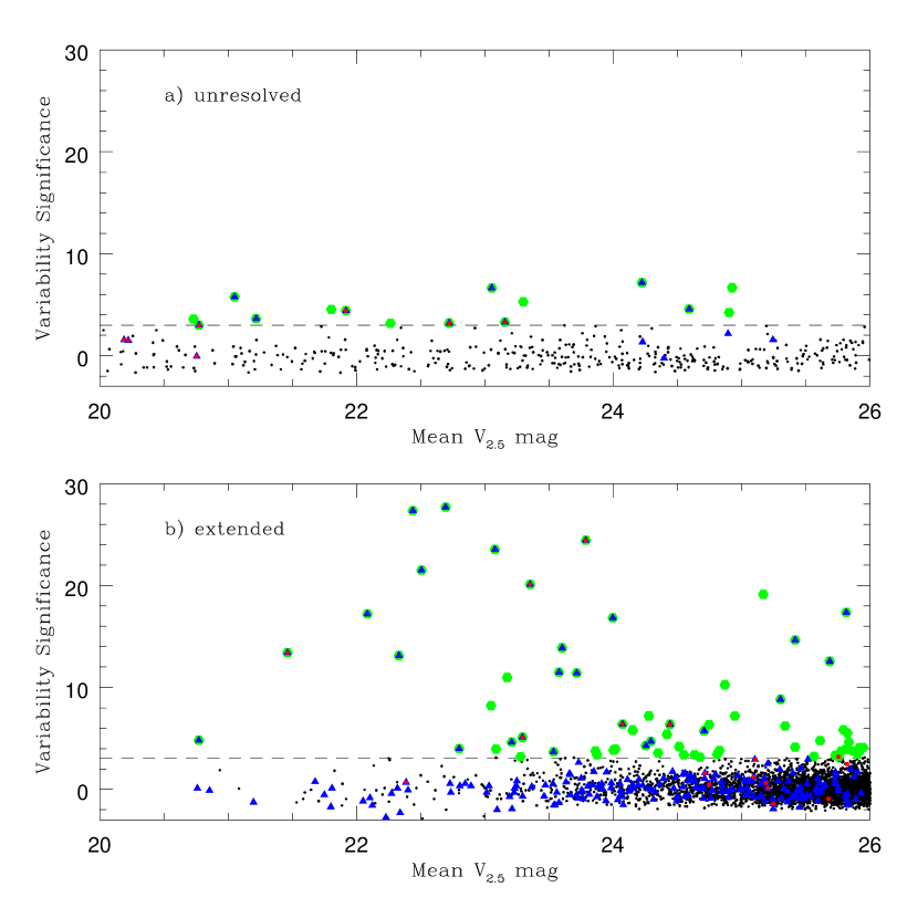
Figure 4: Mean V magnitude vs. variability significance for a) unresolved sources and b) extended sources. The variability significance is the standard deviation with the mean subtracted, divided by 1$\sigma$ from the Gaussian fit to binned standard deviation distributions at each magnitude (see dashed lines in Figure 3). The dashed lines represent the threshold for significant variability (see text and Figure 5). Green points indicate all significantly varying sources (above 3.1$\sigma$ for extended sources and 3.0$\sigma$ for unresolved sources). Blue triangles indicate sources associated with X-ray emission in the 2Ms Chandra surveys. Red squares represent Spitzer mid-IR power-law sources.

The final sample of galaxies surveyed for AGN variability is shown in Figure 4. We normalize the y-axis by dividing the standard deviation of each galaxy (with the mean standard deviation at that magnitude subtracted) by the 1$\sigma$ Gaussian fit determined for the galaxies at each magnitude, the majority of which are assumed to be non-varying. We call this the variability significance parameter. The variability significance will have a value of 3 for objects that are varying by exactly 3 times the 1$\sigma$ Gaussian fit (i.e. spread) in standard deviation values at a given magnitude. Since we subtract off the mean standard deviation, some sources will have negative variability significance values.

To determine the threshold of variability and estimate the number of false positives, we employ an empirical approach. We examine the cumulative distribution of variability signficance values for resolved and unresolved galaxies in GOODS (Figure 5). For a non-varying population, a smooth decline in the distribution should be observed. A population of significant outliers should appear as a break in that distribution with a shallower decline at higher variability significance values. A fit to the distribution of the non-varying sources (long dashed line) helps to identify the break at a significance value of $\sim$3.1 for the extended sources and at $\sim$3 for the unresolved sources (short dashed line). We use this value for the threshold of variability and indicate it with a dashed line in Figure 4. To estimate the number of outliers, we extend the fit to the smooth distribution of non-varying galaxies at low significance values to the y-intercept. Integrating below this line and beyond the variability threshold (shaded region in Figure 5) yields an estimate of the expected number of outliers from the non-varying population. With a total of 3775 extended sources and 399 unresolved sources, the shaded regions represent $\sim$4 false positives among the extended and $\sim$3 false positives among the unresolved sources for a total of 7 expected false positive variables.

Based on our determined variability thresholds, we identify 42 variable galaxies out of a possible 2055 galaxies in the GOODS South field and 43 variables out of 2119 galaxies in the GOODS North field. This represents 2% of all galaxies within the flux limits of the survey that display significantly varying nuclei over the 6 month time interval. We estimate that $\sim$7 of the 85 total variables, or $\sim$8%, are false positives. Table 1 lists the variables identified in the GOODS survey.

2.1 Comparison with Other Variability Surveys in GOODS

Previous studies to identify variables in the GOODS fields or its subregions have been published (Sarajedini et al. 2003; Cohen et al. 2006; Klesman & Sarajedini 2007; Trevese et al. 2008, Villforth et al. 2010). Here we compare our results with Trevese et al. (2008) and Villforth et al. (2010), the two studies with the largest field overlap and data similarities. We discuss Klesman & Sarajedini (2007) in §3 since that study consisted of X-ray and mid-IR pre-selected AGN candidates which we consider in that section of the paper.

The survey with the greatest similarity in terms of photometric data and field coverage is that recently published by Villforth et al. (2010). They identify a variability selected sample of galaxies using the z-band ACS 5 epoch GOODS images. The sample of 139 likely AGN candidates are chosen based upon significant variability using the $C$ statistic, a technique that compares the observed standard deviation to the expected standard deviation for each source. We find that 86 of their 139 candidates are also analyzed for variability in our survey. Those not included in our survey were removed due to the presence of a cosmic ray in or near the nucleus in one or more epochs, the galaxy location being too close to the CCD edge in one or more epochs, or not falling within the magnitude parameters of our survey as defined above. For those sources analyzed in both surveys, we find 23 variables in common or 27%. Villforth et al. divide their sample into a “clean” sample and “normal” sample, where the clean sample consists of sources with $\geq$ 99.99% variability significance and the ”normal” sample contains additional sources down to 99.9% significance. Twenty-two of the variables found in common are in the Villforth et al. (2010) “clean” sample and only 1 is found in the remaining “normal” sample. Considering only the clean sample, 57 of their variables are in our survey and 22 were found to be variable. Thus the percentage of variables in common increases from 27% to 39% if we consider only the most significant variables in their survey.

The sample differences may result from a number of factors. First, the difference in the wavelength of the filter used to identify variables may play a role. We found a larger number of variables and a greater overlap with X-ray surveys in the HDF when analyzing variability in the V-band (Sarajedini et al. 2003) as compared to the I-band (Sarajedini et al. 2000). This is consistent with findings that variability amplitude increases with decreasing wavelength (e.g. Vanden Berk et al. 2004). Secondly, differences in the photometric aperture choice used to identify variability may also be important. We use smaller apertures for the extended sources (r$=$0.125${}^{\prime\prime\,}$ versus their r$=$0.36${}^{\prime\prime\,}$) which should be more sensitive to nuclear flux changes while still remaining largely unaffected by PSF variations (see Villforth et al. 2010, Figure 1). The aperture we use for unresolved sources is actually closer to that adopted by Villforth et al. (2010). We chose a larger aperture for these objects (r$=$0.25${}^{\prime\prime\,}$ and additional tests at r$=$0.5${}^{\prime\prime\,}$) to limit effects from PSF variations. Additional comparisions of these samples are the focus of a future paper.

Another variability study in this field is that of Trevese et al. (2008) in the Chandra Deep Field South which encompases the GOODS-S. The variables were selected from a V-band ground-based survey using the ESO/MPI 2.2m telescope. The observations cover a time baseline of $\sim$2 years and are sampled every few months. They identify 132 variables in this larger field, of which 22 are in the ACS field-of-view. Fourteen of these are included within the parameters of our variability survey. Of these 14, we find 8 as significant variables in our survey or 57%. If we restrict the sample to those which Trevese et al. identify as BLAGNs, we find 80% as variable (8 out of 10).

We identify a higher density of variables in our common field (42 as compared to 14) which is likely due to the differences in image resolution. The high resolution HST images allow us to use small aperture photometry to isolate the varying galaxy nucleus and should be more sensitive to varying AGN. In addition, the image quality and repeatability of the HST data allows for the detection of variability to a lower threshold in terms of standard deviation. The variables identified by Trevese et al. (2008) that are not found in our survey may result from longer and more complete time sampling of the AGN light curve. Our survey covers a 6 month time interval and is expected to be $\sim$60% complete in detecting variable AGN while longer time sampling over 1 to 2 years should identify virtually all varying AGN (e.g. Koo et al. 1986; Schmidt et al. 2010).

3 COMPARISON WITH MULTI-WAVELENGTH SURVEYS

The GOODS North and South fields have been the target of deep X-ray observations with Chandra and mid-IR imaging with Spitzer IRAC and MIPS. We compare AGN candidates selected via X-ray detection and mid-IR power-law SED fitting to our variability selected AGN candidates to investigate their multiwavelength properties and various biases among the different selection techiniques. We also examine evidence for AGN based on emission line properties from published redshift surveys in these fields.

3.1 X-ray Detected AGN

All optical sources surveyed for variability were matched against the list of X-ray point source detections from the 2Ms Chandra Deep Field surveys in the north field (Alexander et al. 2003) and the south (Luo et al. 2008). We refer to the “variability survey” as those optical sources from the GOODS v2.0 catalog that were visible in all 5 epochs with good quality images (i.e. containing no cosmic rays or CCD edge effects) and having nuclear magnitudes brighter than V_2.5$=$26.

In the south field, Luo et al. (2008) found 218 optical matches to the 462 X-ray sources in the main catalog with a matching radius of 0.5${}^{\prime\prime\,}$. We find that 115 of these X-ray/optically matched sources fall within our variability survey. A supplementary catalog, produced with greater sensitivity in the outer regions of the CDF-S due to the inclusion of $\sim$ 250 ks from the E-CDF-S, consists of 86 sources, of which 3 match to sources in the variability survey. A third catalog of bright optical sources with lower X-ray significance detections consists of 30 sources, of which 15 have counterparts in the variability survey. Although most objects in the optically bright catalog are not likely to be AGN based on their low X-ray-to-optical flux ratios, we identify these matches since variability would cast light on the nature of the X-ray emission.

In the north field, Alexander et al. (2003) produced a main source catalog containing 503 sources in the CDF-N, and a bright source catalog containing 75 sources with lower significance X-ray detections matched to optically bright galaxies. Barger et al. (2003) identified optical matches and optical source positions for the main source catalog objects based on ground-based Subaru Suprime-Cam observations (Capak et al. 2003). We match the GOODS-N v2.0 positions to these optical positions rather than the X-ray positions for greater matching accuracy. There are 139 objects in the variability survey with matches to X-ray sources in the main catalog within 0.5${}^{\prime\prime\,}$ of the optical counterpart position given in Barger et al. (2003). Two objects with offsets between 0.5 - 1.0${}^{\prime\prime\,}$ were included as matches since their X-ray positions matched the GOODS-N optical positions within $\sim$0.6${}^{\prime\prime\,}$. Among the bright source catalog, 49 objects match within 0.5${}^{\prime\prime\,}$ of an X-ray source.

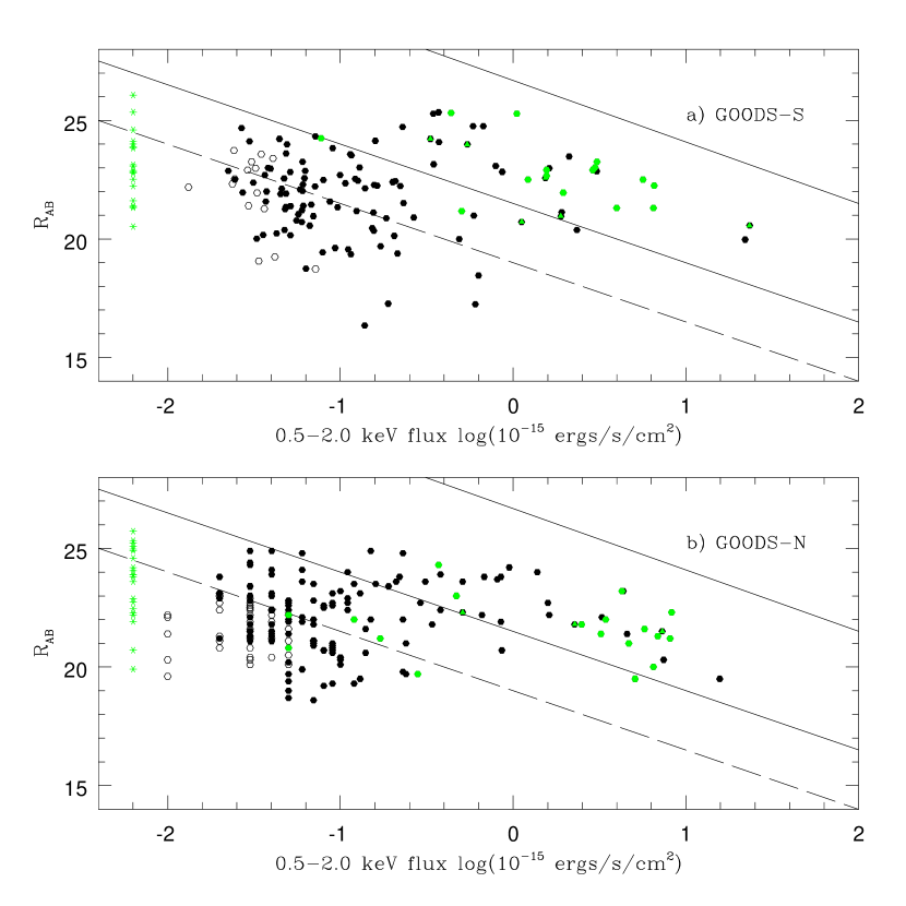
Figure 6: Soft X-ray flux vs. R-band magnitude for objects in a) GOODS south and b) GOODS north. Black points are all X-ray sources with optical counterparts in the variability survey. Green points are those with significant variability (triangles are unresolved objects). The green asterisks are upper limits for non-X-ray detected variables. Solid lines represent log(F_x/F_opt) = -1, +1 and the dashed line is at -2.

We find 21 of the 42 variables in the south field and 21 of the 43 variables in the north field are X-ray detected, yielding a total of 42/85 or 49% of the variables associated with X-ray sources (blue triangles in Fig 4). This fraction is similar to that found in the HDF-N (Sarajedini et al. 2003) and higher than recent ground-based optical variability surveys (Travese et al. 2008; Morokuma et al. 2008) where 60–70% of variables were not detected in X-rays. In Figure 6, we plot the soft band flux (0.5 to 2 keV) against the R-band AB magnitude for all X-ray detected sources in the variability survey. The solid lines indicate the location of most AGN with log($F_{x}/F_{opt}$) between -1 and 1 and the dashed line indicates log($F_{x}/F_{opt}$) = -2. Most non-AGN X-ray sources fall below the dashed line. It can be seen that the majority of bright source catalog objects (open circles) are not likely to be AGN based on their low $F_{x}/F_{opt}$ values. The green points indicate the variable sources. We find that the majority of variables are likely to be AGN based on their location in this diagram but a significant number (19%) have low $F_{x}/F_{opt}$ values. None of the objects in the X-ray bright source catalog for the GOODS-S field were found to be variable and only one from the GOODS-N field (ID 2426) is variable. This object lies close to the limit of likely AGN $F_{x}/F_{opt}$ values.

Figure 6 also shows the R-band magnitude for variables without an X-ray counterpart (green asterisks). These non-X-ray detected variables cover a range of optical magnitudes but tend to be fainter than the X-ray detected variables sources (average R${}_{AB}=$22.1 for X-ray detected sources and 23.3 for non-X-ray detected sources). Thus, in general they are expected to be more difficult to detect at the flux limits of the Chandra survey. The range of optical magnitudes for the non-X-ray detected sources would indicate that if the optical variability is due to the presence of an AGN, they are likely to have low $F_{x}/F_{opt}$ values, similar to what is found for $\sim$20% of the X-ray detected sources. Additionally, since the optical magnitudes represent the total galaxy+AGN light, all of the points on the diagram will have brighter R-band magnitudes than for the AGN component alone, the extent of which depends on the ratio of AGN to host galaxy luminosity. Therefore, some of the X-ray non-detections, may be extremely faint optical AGN that lie below the flux limits of the X-ray survey.

We explore the variable nature of the X-ray detected sources and find that 21 of the 118 X-ray sources in GOODS-S (combining the main and extended CDF-S catalogs) are significant variables. In GOODS-N, 21 of the 140 X-ray sources are significant variables. Thus, 16.3% of the X-ray sources with optical counterparts in the variability survey are identified as significant variables. We do not include the non-variable bright source catalog objects in this statistic since the aim of our paper is to investigate the varying and non-varying AGN population. With the same reasoning, we may also consider X-ray sources below the dashed line in Figure 6 as less likely AGN candidates. Only 2 variables lie below this line in the north field (one very close to the limit) and none in the south field. If we exclude X-ray sources below log($F_{x}/F_{opt}$) = -2, we find 21 of 75 X-ray sources in the south and 19 of 92 in the north are variable, increasing the percentage of X-ray sources with optically varying counterparts to 24%. This percentage is similar to that found in other variability studies. Klesman & Sarajedini (2007) found that 26% of the X-ray source population in the GOODS-S field were optical variables. Since this earlier analysis examined X-ray sources detected in the previously published 1Ms Chandra survey, many of the fainter X-ray sources and those likely to have lower $F_{x}/F_{opt}$ values were already omitted from their sample (see discussion in Klesman & Sarajedini 2007). Of the 21 objects we identify as optically variable X-ray sources, 18 were also identified in Klesman & Sarajedini (2007). Of the three that were not identified in that paper, one was not included in their analysis since it was only detected in the 2Ms survey. The other two fell just below their variability significance threshold.

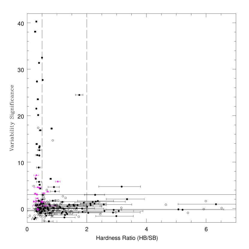
Figure 7: Hardness ratio vs. variability significance for all X-ray sources with optical counterparts. Hardness ratio is defined as the hard X-ray counts (2-7 keV) divided by the soft X-ray counts (0.5-2 keV). Open circles are objects with upper limits only. Magenta triangles are unresolved sources. The dashed lines separate unobscured sources (HR$\leq$0.5) from moderately obscured sources and obscured sources (HR$\geq$2).

We expect that some X-ray detected sources do not reveal significant variability in their optical counterparts due to obscuration. We quantify obscuration using the hardness ratio, HR, defined as the hard band source counts (HB; 2 - 7 keV) divided by the soft band counts (SB; 0.5 - 2 keV). Higher values of HR are found for more obscured sources. Figure 7 shows the hardness ratio vs. the variability significance for all of the X-ray detected sources in our survey with enough counts in either the soft or hard band. Open points are upper limits without enough counts in the hard band to compute a ratio. The solid line shows the threshold above which we consider the source to be significantly varying. As in Klesman & Sarajedini (2007), we find that the majority of variables are ”soft” sources, having HR values less than 0.5. These are also the most significant variables in our sample. We find that 36% of the softest sources are variable, a dramatic increase from the 16% identified as variable overall. The number of optical variables falls significantly among harder, more obscured, X-ray sources. For sources with HR values between 0.5 and 2, we find 8% are optically variable. For the hardest sources with HR values greater than 2, only 1 variable is found accounting for 3% of the X-ray detected sources in our survey. We observe that the variability significance declines with increasing hardness ratio consistent with findings in Klesman & Sarajedini (2007).

We continue to examine the non-X-ray detected variables by performing an X-ray stacking analysis for these sources. The stacking was done for the full, soft and hard bands (Table 2). The last column lists the S/N ratio for the stacked samples. Calculating the source significance instead, the significance for the full, soft and hard bands for the GOODS-N is 1.6$\sigma$, 3.4$\sigma$, and 0$\sigma$, indicating a slightly significant result only for the soft band. For the GOODS-S field, source significance is 2.5$\sigma$, 2.3$\sigma$ and 1.5$\sigma$. The overall results of the analysis are consistent with the trends observed in Figures 6 and 7, that optical variability is more likely to be detected among X-ray soft sources and that many non-X-ray detected variables may emit very weak X-rays and have F_x/F_opt values lower than typical AGN.

The lack of X-ray emission from about half of the sources is not well understood, but is also observed in several previous variability surveys (Trevese et al. 2008, Morokuma et al. 2008). Brandt & Hasinger (2005) discuss some possible explanations (e.g. the lack of an accretion-disk X-ray corona) which may play a role in addition to the possibility that weak X-ray emission is present but not detectable at the current X-ray survey depths.

3.2 IRAC Power-law Detected AGN

Infrared selection of AGN is a powerful technique. Several strategies have been employed using mid-IR observations to identify AGN where some portion of the light has been reprocessed by obsurring dust in the vacinity of the accreting blackhole (e.g. Lacy et al. 2004). Donley et al. (2008) have found that galaxies whose SEDs display power-law behavior in the Spitzer IRAC 3.6 - 8$\mu$m bands represent the purest selection of AGN using mid-IR observations, with many fewer contaminants than IRAC color-color selection or IR-excess AGN selection techniques. We have thus compared our variability selected AGN candidates to the mid-IR power-law galaxies identified in the CDF-N (Donley et al. 2007) and the CDF-S (Alonso-Herrero et al. 2006) which overlap well with the GOODS-N and GOODS-S optical observations.

In the CDF-N, Donley et al. (2007) identified 62 power-law galaxies from the Spitzer IRAC data. Of these, 11 match to optical sources in our variability survey to within 0.7${}^{\prime\prime\,}$. The small overlap in samples is mainly due to the difference in field size and the fact that some IR sources did not fall within the variability survey magnitude limits. Of these 11, 4 are significant optical variables. In the CDF-S, Alonso-Herrero et al. (2006) found 92 power-law galaxies. Of these, 14 match to optical sources in our variability survey and 8 are significant optical variables. In total we find that 48% of the mid-IR power-law galaxies in our survey reveal significant optical variability. This percentage is very similar to that found by Klesman & Sarajedini (2007) for the south field. Mid-IR power-law sources represent 14% of the 85 variables identified in our survey.

We can further study the nature of the optical variables in our survey by investigating the slope of the power-law fit in the Spitzer IRAC 3.6 - 8$\mu$m bands. Power-law galaxies are selected as those sources with IRAC SEDs well fit with f_ν $\sim$ $\nu$^α and having ${\alpha}$ $<$ -0.5. Alonso-Herrero et al. (2006) classify power-law galaxies into catagories based on the slope of the SED, broadly separating the BLAGN-like SEDs from the NLAGN/ULIRG-like SEDs. Steeper (i.e. more negative) values of $\alpha$ more closely match templates of NLAGNs and ULIRGs. Shallower SEDs resemble templates for BLAGNs. These catagories separate at a spectral index of approximately $\alpha$$\simeq$-0.9. From the published power-law slopes for our variables, we find that the majority of mid-IR power-law galaxies which show significant variability have spectral indices similar to BLAGN SEDs (8 out of 12) and those are also the most significantly varying sources. The other third of the variables have steeper SEDs through the IRAC channels and thus would be catagorized as NLAGN or ULIRG-type SEDs.

3.3 Spectroscopically Identified AGN

We compare the variability selected sample to spectroscopically identified AGN in the literature. For the north field, spectroscopic AGN have been identified by Barger et al. (2008) and in the south by Santini et al. (2009). Both papers are compilations of several redshift catalogs referenced within. BLAGNs are classified as sources with clearly broad emission lines while NLAGNs are based on the presence of high ionization emission lines such as [NeV], CIV or CIII]1909.

From these spectroscopic catalogs, we find a total of 27 BLAGNs and 26 NLAGN galaxies that fall within our variability survey. Of those, 20 of the BLAGNs and 4 of the NLAGNs are identified as significant variables. Thus, we find variability in 74% of broad-line AGNs and 15% of narrow-line AGNs previously observed in the GOODS north and south fields. Based on the total number of variables with optical spectroscpic data (see discussion below), we find spectroscopic evidence of AGN in 40% of the variables.

4 GENERAL PROPERTIES OF AGN CANDIDATES AND HOST GALAXIES

Both the north and south GOODS fields have been the target of extensive spectroscopic follow-up. For the south field, we have the spectroscopic catalogs of Szokoly et al. (2004), Cimatti et al. (2002), La Fevre et al. (2004), Vanzella et al. (2008), Mignoli et al. (2005) and Popesso et al. (2009). In the north, we have the compilation of spectroscopic data in Barger et al. (2008) which includes the catalogs of Cowie et al. (2004), Reddy et al. (2006) and Cohen et al. (2000, 2001). For sources without spectroscopic information, photometric redshifts were obtained from the Rainbow Database (Perez-Gonzalez et al. 2008; Guillermo et al. 2010) for the south field and from Fernanez-Soto et al. (1999), Capak et al. (2004), and Bundy et al. (2009) for the north.

Among the 4174 galaxies surveyed for AGN variability in the combined fields, 2371 have spectroscopic redshifts (57%) and an additional 1497 have photometric redshifts yielding redshift information for 93% of the galaxies. Among the 85 variable galaxies, 62 have spectroscopic redshifts (73%) and the remaining 23 have photometric redshifts.

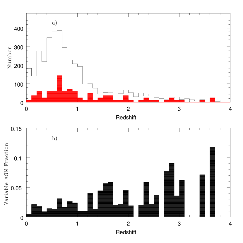
Figure 8: a) Redshift distribution for galaxies in the GOODS variability survey (solid line) and for the significant variables (red shaded histogram) plotted at a scale of 12:1. b) The fraction of galaxies containing a varying nucleus as a function of redshift.

Figure 8a shows the redshift distribution for all galaxies in our survey compared to the distribution of optical variables multiplied by 12 for comparison. The variables have a higher median redshift than the total population with 35 lying at redshifts greater than 1. The percentage of galaxies hosting optically varying nuclei increases with increasing redshift, from $\mathrel{\hbox{\hbox to0.0pt{\hbox{\lower 4.0pt\hbox{$\sim$}}\hss}\hbox{$<$}}}$2% at low redshifts to almost 10% at redshifts greater than 3 (Figure 8b). This is consistent with the fact that the AGN luminosity function shows their numbers peak at redshifts between 0.7$\mathrel{\hbox{\hbox to0.0pt{\hbox{\lower 4.0pt\hbox{$\sim$}}\hss}\hbox{$<$}}}$z$\mathrel{\hbox{\hbox to0.0pt{\hbox{\lower 4.0pt\hbox{$\sim$}}\hss}\hbox{$<$}}}$2, with more luminous AGN peaking at higher redshifts than fainter AGN (e.g. Bongiorno et al. 2007).

To further explore the nature of the AGN candidates, Figure 9 shows redshift vs. rest frame absolute V magnitude for all galaxies in our survey with the variable AGN candidates (green circles), X-ray detected sources (blue triangles), and mid-IR sources (red squares) indicated. We determine rest-frame magnitudes using the v2.0 GOODS catalog b, v, i and z (F435W, F606W, F775W, and F850LP) galaxy photometry (MAG-AUTO) and U-band photometry from Wolf et al. (2004; GOODS-S) and Capak et al. (2004; GOODS-N). These data, together with the redshift information, allows us to compute k-corrected, rest-frame magnitudes and colors for each galaxy in our survey using kcorrect (Blanton et al. 2003).

Figure 9 reveals that AGN candidates generally have brighter optical magnitudes than the non-AGN galaxies. Their luminosity may be partly enhanced by the AGN component, though AGN host galaxies are also typically found to be brighter and more massive than galaxies not hosting AGN (e.g. Brusa et al. 2009). The X-ray detected AGN candidates appear to lie in the brightest galaxies. Mid-IR power-law galaxies cover a range of magnitudes with most lying at the bright end and a few occupying faint galaxies. The mid-IR sources are also generally at higher redshift than the X-ray sources, consistent with other studies of X-ray and mid-IR AGN (Alonso-Herrero et al. 2007). Most optically bright variable AGN candidates are also X-ray sources. The non-X-ray detected optical variables tend to have fainter absolute magnitudes at all redshifts. Thus optical variability appears to identify some intrinisically faint AGN/host galaxies and may do so more efficiently than X-ray or mid-IR AGN identification.

Figure 10 is the color-magnitude diagram for the galaxies in our survey with the same symbols used to identify optical variables, X-ray, and mid-IR sources. We plot the rest-frame U – V color versus the V-band absolute magnitude for galaxies divided into two redshift bins, z=0.2$<$z$<$0.76 and 0.76$<$z$<$1.6. The second bin is more than twice the co-moving volume of the first bin. We see the bimodal color distribution observed in recent surveys (e.g. Hogg et al. 2002) among our survey galaxies. The dashed line indicates the limit of red sequence galaxies as determined in Bell et al. (2004) at the center of each redshift bin.

Several recent findings suggest that the integrated galaxy colors for the AGN candidates in our survey should largely represent the colors of their host galaxies and in most cases are only marginally effected by the light from the nuclear AGN. Recent results by Cardamone et al. (2010) for X-ray selected AGN show little color contamination ($<$0.1 mag) from the nucleus in rest-frame U – V. Likewise, Hickox et al. (2009) find a maximum of 0.4 – 0.5 magnitude color corrections are needed for the bluest AGN sources in (u – r). Exceptions are the most luminous X-ray/optically variable AGN candidates, where we expect the blue colors are indeed significantly affected by the AGN light. These would include several bright (M_V$<$-23) blue optical variables/X-ray sources in the lower left quadrant of Figure 10b.

The AGN galaxy colors cover a range in U–V and fill the region known as the green valley, as observed previously for X-ray detected AGN (e.g. Nandra et al. 2007). Figure 11 shows the color histograms for optical variables, X-ray and mid-IR selected AGN candidates compared to the total galaxy color population. Here we include only galaxies at 0.2$<$z$<$1.6 and correct for the slope of the dashed line in Figure 10. We have also removed the 9 bright, blue sources in the high redshift color magnitude diagram (Fig 10b) that are likely to be affected by the AGN light and may not represent the true host galaxy colors. We find that the X-ray sources and optical variables occupy galaxies at a range of colors, including many within the green valley. While the X-ray sources appear to peak in the green valley, the variables have a flatter distribution that extends blueward of the X-ray host distribution and into the red sequence galaxies. There are few mid-IR AGN candidates at z$<$1.6, but those in this redshift range show a relatively flat distribution. This is consistent with the results of Hickox et al. (2009) who find similar distributions among a sample of 585 AGNs selected via X-ray and mid-IR colors. Recently, Cardamone et al. (2010) found that 75% of X-ray hosts in the green valley have colors consistent with young star-forming galaxies reddened by dust. The blue extension of the optically variable AGN hosts may imply that variability selected AGN are generally less dust reddened. In any case, we find a number of AGN hosts, several identified only through their variable nature, with blue colors indicative of current star formation.

5 DISCUSSION

We have shown that optical variability can be used to identify a significant population of AGN candidates in deep HST fields. The colors and magnitude ranges of the variable hosts are similar to those of other AGN samples selected via X-rays or mid-IR emission but extending to bluer colors and fainter magnitudes. With about 50% of the variables not identified as AGN through other means, we investigate how the inclusion of this population fits with recent theories of AGN/galaxy evolution.

In the current picture of AGN and galaxy evolution, dark matter halos grow in the early universe to masses of 10¹² to 10¹³ M${}_{\hbox{$\odot$}}$ when a dramatic event (e.g. major merger) triggers luminous quasar activity and rapid growth of the central black hole producing a dynamically hot stellar bulge component in the host galaxy (Hopkins et al. 2008; 2009). Other events such as disk instabilities may also trigger accretion onto the black hole and grow the stellar bulge. After this period of growth, star formation in the galaxy must be quenched in order to produce the observed population of passively evolving galaxies on the red sequence. There has been speculation that the quenching results from the event that fuels the quasar and/or is related to radiative feedback during the powerful AGN phase (Alexander et al. 2005; Brand et al. 2006). The high virial temperature of the dark matter halo should stop accretion of cold gas and thus inhibit further star formation (e.g. Faber et al. 2007). The transition of blue, star forming galaxy to a galaxy on the red sequence occurs relatively quickly (1 – 2 Gyr; Barger et al. 1996) which is supported by the dichotomy of observed galaxy colors seen here and in other surveys. There is some evidence that further accretion onto the SMBH occurs during this transition and would explain the observed ”green” colors of X-ray selected AGN (Schawinski et al. 2007), though recent results suggest that many of those may actually be dust reddened star forming galaxies (Cardamone et al. 2010b). Galaxies on the red sequence may continue to experience quenched star formation due to mechanical feedback from the AGN which prevents the accretion of cool gas onto the SMBH (Churazov et al. 2002).

Optical variability is a ubiquitous observational characteristic of accretion onto the SMBH and thus we might expect to identify AGN in the full range of evolutionary stages described above. However, since the variability likely originates from the UV/optically bright accretion disk, variability selection should be most sensitive to unobscured, less dust-reddened AGNs which is largely consistent with our findings. The variables that are also X-ray and mid-IR sources have luminosities, redshifts, and host galaxy colors consistent with the findings of Hickox et al. (2009). Using the observed colors, clustering properties, and SMBH accretion rates, they speculate that the X-ray selected AGN observed at 0.25$<$z$<$0.8 live in large dark matter halo galaxies that have recently experienced the buildup of their bulges and quenching of star formation. These galaxies also exhibit a range of Eddington ratios (10^-3 to 1) which would indicate declining accretion rates onto the SMBH. The mid-IR AGNs in their study are associated with galaxies having less massive dark matter halos and higher Eddington ratios than the X-ray selected sample. Thus, these galaxies have not reached the critical halo mass for the quenching of star formation and therefore are more commonly found in blue host galaxies. Though we do not examine the clustering properties of the different samples here, the colors and magnitudes of the X-ray selected and mid-IR selected variables in our survey would appear to be consistent with this interpretation.

To further investigate the variable AGN candidates found in our survey and attempt to understand their placement in the above evolutionary scenario, we estimate the black hole masses and accretion rates for the variability selected AGN candidates at redshifts less than z$<$1.6. Higher redshift data are excluded in this analysis to avoid the high luminosity AGN which may contaminate galaxy colors and bulge estimates for the host. To determine Eddington ratios however, we first need to estimate the luminosity of the AGN. We expect the AGN component to be $\sim$10% or less of the total galaxy flux in most cases. This is based on the observed variability in the nucleus compared with that expected from AGN structure function flux amplitudes at time intervals similar to our data (e.g. Butler et al. 2010). Nonetheless, we can make a crude estimate of the AGN flux by measuring the nuclear magnitude within r=0.125${}^{\prime\prime\,}$ apertures, twice the FWHM for the ACS images. This aperture contains the highest concentration of the AGN light and represents an upper limit on the AGN luminosity since this measurement will contain essentially all of the AGN plus some underlying flux from the host galaxy. The nuclear V-band magnitudes are converted to rest-frame B-band absolute magnitudes. We use the bolometric corrections of Hopkins et al. (2007) to convert to bolometric luminosity. Figure 12a shows the upper limit bolometric luminosity versus redshift for the variables at z$<$1.6 where X-ray detected variables are shown as black points and non-X-ray detected variables are green. We find that the upper limit bolometric luminosities for non-X-ray detected variables are generally fainter than that for the X-ray selected sample at all redshifts but with a large dispersion.

To estimate black hole masses, we compute the stellar bulge masses for our variable galaxies. We used GALFIT (Peng et al. 2002) to fit a 2-component model consisting of an exponential disk and n$=$4 sersic profile bulge in both the V(F606W) and i-band(F775W) images. Fits with an n$=$2 sersic bulge were also computed but showed no significant differences with the n$=$4 fits. With the magnitudes for each component determined, we then calculated the total galaxy and bulge masses using the color and galaxy redshift. Reliable bulge masses were calculated for 48 of the 62 variable galaxies at z$<$1.6 using this technique. In some cases a significant bulge component was not identified in one of the bands, making a bulge mass measurement impossible. We use the relation from Marconi & Hunt (2003) to convert bulge mass to black hole mass and plot this as a function of redshift in Figure 12b. The variables have a range of black hole masses with an average of 7.2 log(M_BH[M${}_{\hbox{$\odot$}}$]). There is no apparent difference between the non-X-ray and X-ray detected variables at z$<$1. At higher redshifts, the non-X-ray detected variables appear to have lower mass black holes in general, though the number of sources at these redshifts with reliable bulge measurements is fewer. We note that any significant contribution by the AGN component could produce an artificially high bulge mass and consequently overestimate the black hole mass. While we expect the contribution of the AGN component to be negligible in the majority of our sources, the higher redshift and X-ray detected sources are more likely to be susceptible to this effect based on their overall colors and luminosities (as discussed in $\S$4). This may account for the slightly higher BH masses for z$>$1 variables that are also X-ray detected in Figure 12b.

Finally, we compute the Eddington ratios using the equation L_Edd = 1.3 $\times$ 10³⁸ (M_BH/M${}_{\hbox{$\odot$}}$) erg/s. Figure 12c shows the Eddington ratio as a function of redshift. Several sources at z$>$1 have luminosities brighter than Eddington which is likely caused by the fact that our bolometric luminosity is an upper limit. Thus, these values are less reliable estimates of the true Eddington ratios of these sources. Nonetheless, we find no discernible difference among the X-ray and non-X-ray detected variable AGN across the range of observed redshifts.

These results suggest that the hosts of variability-detected AGN comprise a mix of galaxy-AGN types. Some of the variables appear to be similar to other X-ray selected sources, having hosts with significant stellar bulges and recently quenched star formation, followed by a decline in the accretion rate onto the black hole (Hickox et al. 2009). In other cases the SMBHs may be continuously or stochastically fueled, possibly at lower levels by stellar winds or bars in disk galaxies. Such systems could have slightly higher Eddington ratios and be in intermediate mass, later-type hosts (Hopkins et al. 2009) much like the mid-IR/optical AGN discussed in Hickox et al. (2009). This scenario would be consistent with the observed lower-luminosity AGN within bluer host galaxies.

6 CONCLUSIONS

We have conducted a variability survey for AGN candidates in the GOODS fields and compared this selection technique with results from other multiwavelength surveys of these fields. Using small aperture photometry, we identify 85 galaxies with significantly varying nuclei in the HST ACS V-band images. This represents 2% of all galaxies surveyed to a limiting magnitude of V_2.5=26 with an estimated 7 false positives. Forty-two of the 85 variables are associated with X-ray sources detected in the Chandra 2Ms surveys of these fields and 14 of the variables have power-law SEDs through the Spitzer IRAC mid-IR bands. All but one of the mid-IR sources is also an X-ray source, resulting in a total of 43 of 85 variables (51%) with additional multiwavelength evidence for the presence of an AGN. Optical variability is more sensitive to soft X-ray sources with fewer optical variables found to be associated with the harder X-ray detected sources in these fields. This is consistent with the results of X-ray stacking for the non-X-ray detected variables which reveals a marginally significant detection in the soft X-ray band (0.5–2 keV) only. We also find that the slope of the power-law fit through the mid-IR bands for optical variables is consistent with BLAGN-like SEDs for 2/3rds of the variable AGN candidates with the other third having steeper slopes like those for NLAGNs and ULIRGs. Likewise, among spectroscopically identified AGN, 74% of BLAGNs and 15% of NLAGNs show optical variability.

Our findings indicate that optical variability most efficiently identifies less obscured, Type I - like AGN, though a surprisingly significant fraction (15 – 30%) appear to have some degree of obscuration revealed through the lack of an observed broad-line region, slightly harder X-ray emission, or the slope of the mid-IR SED. The overall number density of variable AGN candidates is about half that of likely AGN X-ray sources with optical counterparts in the GOODS fields and almost 3 times that of mid-IR power-law AGN with optical counterparts. Thus, variability uncovers a significant population of AGN which complements detection methods at other wavelengths.

The variable AGN candidates span a broad range in redshift with the percentage of galaxies hosting variable nuclei increasing from $\mathrel{\hbox{\hbox to0.0pt{\hbox{\lower 4.0pt\hbox{$\sim$}}\hss}\hbox{$<$}}}$2% at low redshift to $\sim$10% at z$\sim$3. The total galaxy+AGN absolute magnitudes reveal that AGN candidates (variable, X-ray and mid-IR detected candidates) are generally found in brighter galaxies at a range of colors spanning that of the total galaxy population. The color distribution of X-ray detected AGN hosts reveals a peak in number density between the blue, star-forming and red sequence galaxies. The variables follow a similar trend but with an extension towards bluer colors and fainter absolute magnitudes.

Based on the derived bolometric luminosities, BH masses and Eddington ratios for the variable galaxies in our survey, we find that non-X-ray detected variables at z$<$1.6 generally have lower luminosities than X-ray detected variables, but similar BH masses and Eddington ratios. Thus, some of the variables have characteristics like other X-ray selected samples, revealing significant bulges and the onset of quenched star formation and decreased BH accretion rates, while others may be intermediate mass systems still forming stars and accreting at a continuous, lower-level, possibly through stellar winds or bars.

The results of this survey suggest that variability is a promising technique to identify samples of AGN extending to low-luminosities out to z$\sim$3. These results are especially encouraging in light of future planned multi-epoch observing programs like that for the LSST. Observations with longer and better sampled light curves will produce more robust and complete variability-selected AGN samples in the low-luminosity, z$>$1 regime comparable to the well-quantified light curves and structure functions for QSOs (e.g. MacLeod et al. 2010). Together with multiwavelength surveys using a variety of detection techniques, the AGN population can be more powerfully probed and understood in the context of galaxy evolution.

Figure 1: Mean V magnitude vs. standard deviation for all sources in the the GOODS-N (squares) and GOODS-S (asterisks) fields with a) r$=$2.5 pixel photometry and b) r$=$5 pixel photometry. Average V magnitude vs. concentration index (V_2.5 - V₅) is shown in panel c, where the dashed line represents the separation between resolved/extended sources and unresolved/point-like sources. All sources have 5 magnitude measurements from which the standard deviation was determined.

Figure 2: Mean V magnitude vs. standard deviation for all sources in the the GOODS-N (squares) and GOODS-S (asterisks) fields. a) unresolved sources and b) resolved sources shown using r$=$2.5 pixel photometry. c) unresolved sources and d) resolved sources shown using r$=$5 pixel photometry.

Figure 3: Mean V magnitude vs. standard deviation for a) unresolved sources in GOODS-S, b) extended sources in GOODS-S, c) unresolved sources in GOODS-N, d) extended sources in GOODS-N. Mean V magnitudes are measured within r$=$2.5 pixel apertures. Standard deviation values are calculated using r$=$2.5 pixel apertures for extended sources and r$=$5 pixel apertures for unresolved sources. The solid line is a fit to the center of the distribution of standard deviation values as a function of magnitude. The dashed lines represent the mean plus 2$\sigma$ and mean plus 3$\sigma$ standard deviation values, where $\sigma$ is determined from the Gaussian fit to the binned standard deviation distributions at each magnitude.

Figure 5: Variability significance cumulative histogram for a) unresolved sources and b) extended sources (solid line). The long dashed line represents a fit to the distribution at low significance values ($\mathrel{\hbox{\hbox to0.0pt{\hbox{\lower 4.0pt\hbox{$\sim$}}\hss}\hbox{$<$}}}$3). The short dashed line is the approximate break of the distribution from the low significance distribution fit (i.e. at values higher than this threshold, we consider the source to be significantly varying beyond the normal galaxy population). The shaded region represents the expected false positive population among the significantly varying sample ($\sim$3 sources among the unresolved sources and $\sim$4 sources among the extended sources).

Figure 9: Redshift vs. rest-frame absolute V magnitude for all galaxies (black points), optical variables (green circles), X-ray sources (blue triangles) and mid-IR power-law sources (red squares).

Figure 10: Color-magnitude diagram for GOODS galaxies at a) 0.2$<$z$<$0.76 and b) 0.76$<$z$<$1.6. Symbols are as in Fig 9. Dashed lines represent the lower limit of red sequence galaxies at the average redshift for each panel (Bell et al. 2004).

Figure 11: Galaxy color histograms for all galaxies at z$<$1.6 in GOODS (solid line in all panels). a) variability selected AGN hosts (green), b) X-ray selected AGN hosts (blue), and c) mid-IR power-law selected AGN hosts at z$<$1.6.

Figure 12: a) Bolometric luminosity, b) black hole mass, and c) Eddington ratio vs redshift for variable galaxies at z$<$1.6. Black points are variables that are also X-ray sources and green points indicate non-X-ray detected variables.

Table 1: Variable Nuclei Galaxies in GOODS

GOODS ID	RA	DEC	V2.5	CI	Std Dev	Significance	Redshift	ph/sp	Note	X-ray/IR AGN
263	188.9272156	62.2081223	25.730	0.946	0.084	3.365	0.440	ph	6	–
1177	188.9713287	62.1769981	22.330	0.210	0.047	3.127	1.381	sp	2	X-ray
3164	189.0242615	62.1966934	24.708	0.418	0.072	5.745	1.485	sp	2	X-ray
6370	189.0749664	62.2763901	21.770	0.242	0.090	2.488	0.580	ph	6	X-ray
6527	189.0774994	62.1875343	22.506	0.214	0.073	1.511	1.020	sp	1	X-ray
7321	189.0874634	62.2367172	25.302	0.298	0.134	8.833	1.530	ph	6	X-ray
8848	189.1068878	62.2799873	24.826	0.350	0.058	3.821	2.000	ph	6	–
9104	189.1100006	62.1646309	25.776	0.924	0.092	3.773	0.840	sp	1	–
9345	189.1127319	62.2994232	24.676	0.660	0.048	3.166	1.680	ph	6	–
9386	189.1133118	62.1260033	24.746	0.972	0.079	6.356	0.321	sp	1	–
10066	189.1220245	62.2704849	24.292	0.676	0.051	4.720	0.850	sp	1	X-ray
11426	189.1384735	62.1429482	22.658	0.314	0.127	38.092	0.934	sp	2	X-ray
12198	189.1471252	62.1860580	23.208	0.638	0.031	4.633	0.409	sp	1	X-ray
13302	189.1590424	62.1154747	25.564	0.672	0.076	3.258	3.650	ph	6	–
14163	189.1684875	62.1062279	25.864	0.660	0.096	3.776	2.350	ph	6	–
15439	189.1825867	62.1221237	25.918	0.748	0.104	4.121	1.990	ph	6	–
16346	189.1929932	62.2707367	25.812	1.274	0.096	3.931	0.503	sp	2	–
18014	189.2113037	62.1388969	25.824	0.458	0.121	5.531	1.519	sp	1	–
21365	189.2451630	62.2430305	23.716	0.528	0.074	11.415	0.677	sp	2	X-ray
24210	189.2760620	62.3601723	22.628	0.228	0.132	40.276	0.904	sp	1	X-ray
24637	189.2812042	62.3632812	23.220	0.232	0.138	31.371	1.450	sp	2	X-ray
25631	189.2930145	62.3034363	24.002	0.350	0.039	3.865	0.697	sp	1	–
26715	189.3054657	62.3478355	25.612	0.718	0.099	4.781	0.180	ph	6	–
26774	189.3061218	62.3603401	24.350	1.102	0.044	3.583	0.275	sp	-	-
27941	189.3194733	62.2925835	24.442	0.360	0.068	6.385	1.146	sp	1	X-ray,IR
28356	189.3245087	62.3154716	23.292	0.254	0.034	5.112	2.237	sp	2	X-ray,IR
30926	189.3559875	62.2489471	25.922	0.346	0.099	3.795	2.545	sp	3	–
30987	189.3569031	62.2801285	20.770	0.316	0.024	4.832	0.000	sp	1	X-ray
32037	189.3706360	62.1909637	25.168	0.544	0.242	19.125	0.810	ph	6	–
32542	189.3768311	62.2312050	25.416	0.334	0.082	4.150	1.600	ph	6	–
34017	189.3970337	62.3355713	24.152	0.644	0.055	5.822	1.083	sp	2	–
35004	189.4146118	62.2506256	25.836	1.108	0.108	4.640	0.821	sp	1	–
2426	189.0090942	62.2106133	23.862	0.560	0.036	3.767	0.639	sp	2	X-ray
4680	189.0501404	62.1941376	22.694	0.934	0.097	27.694	0.276	sp	2	X-ray
4809	189.0520020	62.1945724	23.279	0.724	0.026	3.216	0.276	sp	1	–
7902	189.0950012	62.2166138	22.798	0.652	0.025	3.987	0.473	sp	2	X-ray
10848	189.1320648	62.1311073	24.948	0.426	0.096	7.200	1.790	ph	6	–
17767	189.2086639	62.1337738	25.900	1.248	0.093	3.480	0.559	sp	1	–
22976	189.2613525	62.2621117	22.084	0.378	0.055	17.224	0.512	sp	2	X-ray
23832	189.2719421	62.2962265	24.810	0.558	0.054	3.448	0.789	sp	2	–
1667	188.9900970	62.1734390	23.052	0.196	0.120	6.635	3.075	sp	2	X-ray
35757	189.4272003	62.3033028	21.918	0.180	0.090	4.435	2.309	sp	2	X-ray,IR
38313	189.4888000	62.2742996	22.722	0.178	0.072	3.197	2.922	sp	1	X-ray,IR
820	53.0084343 -	27.7590332	25.946	0.616	0.105	4.099	1.899	ph	4	–
2967	53.0344429 -	27.6982098	25.816	0.246	0.298	17.375	2.470	sp	4	X-ray
4234	53.0454674 -	27.7374840	23.352	0.256	0.107	20.128	1.615	sp	4	X-ray,IR
6038	53.0586662 -	27.7084370	25.418	0.226	0.204	14.668	2.026	sp	5	X-ray
6254	53.0601578 -	27.7734680	24.416	0.544	0.053	5.406	0.734	sp	4	–
6595	53.0624199 -	27.8575153	24.254	0.622	0.042	4.300	0.675	sp	4	X-ray
8830	53.0767479 -	27.8174648	24.548	0.818	0.042	3.396	0.261	sp	5	–
9055	53.0782013 -	27.8784523	25.794	0.790	0.122	5.831	0.910	ph	4	–
10019	53.0842857 -	27.8140373	24.018	0.808	0.036	3.969	0.735	sp	4	–
11674	53.0942993 -	27.8534985	24.868	0.774	0.110	10.266	0.990	ph	4	–
13494	53.1048546 -	27.7052193	24.072	0.252	0.051	6.415	1.617	sp	4	X-ray,IR
14049	53.1079750 -	27.7337475	23.086	0.530	0.031	3.957	0.278	sp	4	–
15416	53.1146431 -	27.9367771	25.338	0.612	0.098	6.226	0.663	sp	5	–
17366	53.1249123 -	27.7583027	21.462	0.202	0.076	13.403	1.215	sp	4	X-ray,IR
17438	53.1252556 -	27.7565346	23.602	0.230	0.080	13.885	0.955	sp	4	X-ray
17558	53.1259003 -	27.7512760	22.438	0.214	0.141	27.362	0.735	sp	4	X-ray
18648	53.1315727 -	27.7702045	24.634	0.840	0.044	3.402	0.680	ph	4	–
18812	53.1324959 -	27.8528843	23.048	0.202	0.051	8.213	0.400	ph	4	–
19698	53.1375771 -	27.7001095	25.754	0.318	0.081	3.211	1.236	sp	5	IR
23092	53.1560745 -	27.6666927	23.578	0.288	0.068	11.501	0.664	sp	4	X-ray
24366	53.1636200 -	27.7053509	24.276	0.410	0.061	7.212	1.764	sp	5	–
26093	53.1744499 -	27.7332993	25.686	0.222	0.209	12.566	0.381	sp	5	X-ray
26882	53.1801491 -	27.8206043	23.240	0.230	0.293	59.702	1.920	sp	4	X-ray,IR
29404	53.2007370 -	27.8823910	23.534	0.614	0.030	3.686	0.667	sp	4	X-ray
29808	53.2045441 -	27.8972778	24.512	0.702	0.047	4.200	0.419	sp	4	–
31429	53.2203522 -	27.8555088	23.996	0.332	0.108	16.851	1.220	sp	4	X-ray
7929	53.0714340 -	27.7175846	23.078	0.736	0.123	23.532	0.566	sp	4	X-ray
15508	53.1150970 -	27.6958046	23.786	0.516	0.139	24.456	0.665	sp	4	X-ray,IR
15694	53.1161232 -	27.8933048	23.872	0.270	0.031	3.401	0.621	sp	5	–
18828	53.1325912 -	27.8529434	23.172	0.212	0.064	10.979	2.796	sp	5	–
1872	53.0232468 -	27.7772713	22.264	0.196	0.073	3.190	0.710	ph	4	–
8701	53.0760040 -	27.8781586	24.592	0.194	0.123	4.567	2.801	sp	4	X-ray
14887	53.1119652 -	27.7132568	24.902	0.198	0.124	4.238	0.804	ph	4	–
22530	53.1528091 -	27.8778725	24.926	0.174	0.173	6.670	0.620	ph	4	–
23424	53.1580276 -	27.7691936	20.728	0.162	0.073	3.609	0.150	ph	4	–
23556	53.1588287 -	27.6624470	20.772	0.164	0.065	3.008	0.837	sp	4	X-ray,IR
24251	53.1628609 -	27.7671623	21.218	0.158	0.074	3.624	1.216	sp	4	X-ray
26077	53.1743851 -	27.8673534	23.156	0.178	0.080	3.296	3.610	sp	4	X-ray,IR
26512	53.1775360 -	27.9149456	21.804	0.186	0.090	4.534	0.120	ph	4	–
27457	53.1846352 -	27.8809185	24.224	0.188	0.163	7.162	3.471	sp	4	X-ray
29365	53.2003708 -	27.7898388	23.298	0.182	0.114	5.287	0.700	ph	4	–
3485	53.0393639 -	27.8018875	21.048	0.168	0.102	5.786	2.810	sp	4	X-ray

Note. — 1 - Barger et al. 2008, 2 - Wirth et al. 2008, 3 - Reddy et al. 2006, 4 - Barro et al. 2010, 5 - Popesso et al. 2009, 6 - Bundy et al. 2009

Table 2: X-Ray Stacking Results

Energy Band (keV)	No. Stacked Sources	Total Counts	Total Background Counts	S/N
GOODS-N
0.5 - 0.7	20	228 $\pm$ 15	205.1 $\pm$ 0.5	1.5
0.5 - 2.0	20	96 $\pm$ 10	67.7 $\pm$ 0.3	2.9
2.0 - 7.0	19	127 $\pm$ 11	130.3 $\pm$ 0.4	-0.3
GOODS-S
0.5 - 0.7	19	273 $\pm$ 17	234.1 $\pm$ 0.5	2.4
0.5 - 2.0	20	99 $\pm$ 10	78.4 $\pm$ 0.3	2.1
2.0 - 7.0	18	170 $\pm$ 13	152.0 $\pm$ 0.4	1.4

References

- (1)
- (2) Alexander, D. M., et al. 2003, AJ, 126, 539
- (3)
- (4) Alexander, D. M., Bauer, F. E., Chapman, S. C., Smail, I., Blain, A. W., Brandt, W. N.,& Ivison, R. J. 2005, ApJ, 632, 736
- (5)
- (6) Alonso-Herrero, A., et al. 2006, ApJ, 640, 167
- (7)
- (8) Baldwin, J. A., Phillips, M. M. & Terlevich, R. 1981, PASP, 93, 5
- (9)
- (10) Barger, A. J., Aragon-Salamanca, A., Ellis, R. S., Couch, W. J., Smail, I., & Sharples, R. M. 1996, MNRAS, 279, 1
- (11)
- (12) Barger, A. J., Cowie, L. L., Capak, P., Alexander, D. M., Bauer, F. E., Brandt, W. N., Garmire, G. P., & Hornschemeier, A. E. 2003, ApJL, 584, 61
- (13)
- (14) Barger, A. J., Cowie, L. L., & Wang, W.-H. 2008, ApJ, 689, 687
- (15)
- (16) Barro, G., et al. 2010, submitted
- (17)
- (18) Becker, R. H., Gregg, M. D., Hook, I. M., McMaon, R. G., White, R. L., & Helfand, D. J. 1997, ApJ, 79, L93
- (19)
- (20) Bell E. F. et al., 2004, ApJ, 608, 752
- (21)
- (22) Bershady, M. A., Trevese, D., & Kron, R. G. 1998, ApJ, 496, 103
- (23)
- (24) Blanton, M. R., Brinkmann, Csabai, I., Doi, M., Eisenstein, D., Fukugita, M., Gunn, J. E., Hogg, D., & Schlegel, D. J. 2003, AJ, 125, 2348
- (25)
- (26) Bongiorno, A., et al. 2007, A&A, 472, 443
- (27)
- (28) Brand, K. et al. 2006, ApJ, 644, 143
- (29)
- (30) Brandt, W. N. & Hasinger, G. 2005, ARA&A, 43, 827
- (31)
- (32) Brusa, M., et al. 2009, A&A, 507, 1277
- (33)
- (34) Bundy K., Fukugita, M., Ellis, R. S.;,Targett, T. A., Belli, S., & Kodama, T. 2009, ApJ, 697, 1369
- (35)
- (36) Butler, N. R. & Bloom, J. S. 2010, arXiv:1008:3143
- (37)
- (38) Capak, P., et al. 2004, AJ, 127, 180
- (39)
- (40) Cardamone, C. N., et al. 2010a, arXiv:1008.2974
- (41)
- (42) Cardamone, C. N., Urry, M., Schawinski, K., Treister, E., Brammer, G., & Gawiser, E. 2010b, arXiv:1008.2971
- (43)
- (44) Cimatti A., Cassata, P., Pozzetti, L., et al. 2008, A&A, 482, 21
- (45)
- (46) Cohen, J. G., et al. 2001, AJ, 121, 2895
- (47)
- (48) Cohen, J. G., et al. 2000, ApJ, 538, 29
- (49)
- (50) Cohen, S. H., et al. 2006, ApJ, 639, 731
- (51)
- (52) Cowie, L. L., Barger, A. J., Hu, E. M., Capak, P., & Songaila, A. 2004, AJ, 127, 3137
- (53)
- (54) Churazov, E., Sunyaev, R., Forman, W., & B hringer, H. 2002, MNRAS, 332, 729
- (55)
- (56) Donley, J. L., Rieke, G. H., Perez-Gonzalez, P. G., Rigby, J. R., & Alonso-Herrero, A. 2007, ApJ, 660, 167
- (57)
- (58) Donley, J. L., Rieke, G. H., Perez-Gonzalez, P. G., Barro, G. 2008, ApJ, 687, 111
- (59)
- (60) Fabbiano, G., Kim, G. W., & Trinchieri, G. 1992, ApJS, 80, 531
- (61)
- (62) Faber, S. M. et al. 2007, ApJ, 665, 265
- (63)
- (64) Fernanez-Soto, A., Lanzetta, K. M., & Yahil, A. 1999, ApJ, 513, 34
- (65)
- (66) Ferrarese, L. & Merritt, D. 2000, ApJL, 539, 9
- (67)
- (68) Gebhardt, K., Bender, R., Bower, G., Dressler, A., Faber, S. M., Filippenko, A. V., Green, R., Grillmair, C., Ho, L. C., Kormendy, J., Lauer, T. R., Magorrian, J., Pinkney, J., Richstone, D., & Tremaine, S. 2000, ApJL, 539, 13
- (69)
- (70) Hickox, R. C., et al. 2009, ApJ, 696, 891
- (71)
- (72) Hogg, D. W., et al. 2002, AJ, 124, 646
- (73)
- (74) Hook, I. M., McMahon, R. G., Boyle, B. J. & Irwin, M. J., 1994, MNRAS, 268, 305
- (75)
- (76) Hopkins, A. M. & Beacom, J. F. 2006, ApJ, 651, 142
- (77)
- (78) Hopkins, P. F., Richards, G. T., & Hernquist, L. 2007, ApJ, 654, 731
- (79)
- (80) Hopkins, P. F., Hernquist, L., Cox, T. J., & Kere, D. 2008, ApJS, 175, 356
- (81)
- (82) Hopkins, P. F., Cox, T. J., Younger, J. D., & Hernquist, L. 2009, ApJ, 691, 1168
- (83)
- (84) Klesman, A. & Sarajedini, V. L. 2007, ApJ, 665, 225
- (85)
- (86) Koo, D., Kron, R., & Cudworth, K. 1986, PASP, 98, 285
- (87)
- (88) Kormendy, J., & Richstone, D. 1995, ARA&A, 33, 581
- (89)
- (90) Lacy, M., et al. 2004, ApJS, 154, 166
- (91)
- (92) La Fevre, O., et al. 2004, A&A, 428, 1043
- (93)
- (94) Luo, B., et al. 2008, ApJS, 179, 19
- (95)
- (96) MacLeod, C. L., et al. 2010, ApJ, 721, 1014
- (97)
- (98) Marconi, A. & Hunt, L. K. 2003, ApJL, 589, 21
- (99)
- (100) Markarian, B. E. 1967, Astrofizika, 3, 55
- (101)
- (102) Mignoli, M., et al. 2005, A&A, 437, 883
- (103)
- (104) Morokuma, T., et al. 2008, ApJ, 676, 121
- (105)
- (106) Nandra, K. et al. 2007, ApJL, 660, 11
- (107)
- (108) Peng, C. Y., Ho, L. C., Impey, C. D., & Rix, H. 2002, AJ, 124, 226
- (109)
- (110) Pereya, N. A., Vanden Berk, D. E., Turnshek, D. A., Hillier, D. J., Wilhite, B. C., Kron, R. G., Schneider, D. P., & Brinkmann, J. 2006, ApJ, 642, 87
- (111)
- (112) Perez-Gonzalez, P. G., et al. 2008, ApJ, 675, 234
- (113)
- (114) Popesso, P., et al. 2009, A&A, 494, 443
- (115)
- (116) Reddy, N. A., Steidel, C. C., Erb, D. K., Shapley, A. E., & Pettini, M. 2006, ApJ, 653, 1004
- (117)
- (118) Richards, G. T., et al. 2002, AJ, 123, 2945
- (119)
- (120) Rigby, J. R., Rieke, G. H., Donley, J. L., Alonso-Herrero, A., & P rez-Gonz lez, P. G. 2006, ApJ, 645, 115
- (121)
- (122) Santini, P., et al. 2009, A&A, 504, 751
- (123)
- (124) Sarajedini, V. L., Gilliland, R. L., & Phillips, M. M. 2000, AJ, 120, 2825
- (125)
- (126) Sarajedini, V. L., Gilliland, R. L., & Kasm, C. 2003, ApJ, 599, 173
- (127)
- (128) Sarajedini, V. L., et al. 2006, ApJS, 166, 69
- (129)
- (130) Schawinski, K., et al. 2007, MNRAS, 382, 1415
- (131)
- (132) Schmidt, M. & Green, R. F. 1983, ApJ, 269, 352
- (133)
- (134) Schmidt, K., Marshall, P. J., Rix, H.-W., Jester, S., Hennawi, J. F., & Dobler, G. 2010, ApJ, 714, 1194
- (135)
- (136) Smith, M. G. & Wright, A. E. 1980, MNRAS, 191, 871
- (137)
- (138) Stern, D., et al. 2005, ApJ, 631, 163
- (139)
- (140) Szokoly, G. P., et al. 2004, ApJS, 155, 271
- (141)
- (142) Trevese, D., Boutsia, K., Vagnetti, F., Cappellaro, E. & Puccetti, S. 2008, A&A, 488, 73
- (143)
- (144) Vanden Berk, D. E., et al. 2004, ApJ, 601, 692
- (145)
- (146) Vanzella, E., Cristiani, S., Dickinson, M., et al. 2008, A&A, 478, 83
- (147)
- (148) Veilleux, S. & Osterbrock, D. E. 1987, ApJS, 63, 295
- (149)
- (150) Villforth, C., Koekomoer, A. M., & Grogin, N. A. 2010, arXiv:1008:3384
- (151)
- (152) Webb, W. & Malkan, M. 2000, ApJ, 540, 652
- (153)
- (154) Wolf, C., Hildebrandt, H., Taylor, E. N., Meisenheimer, K. 2008, A&A, 492, 933
- (155)
- (156) Wolf C., et al. 2004, A&A, 421, 913
- (157)