Prime numbers: periodicity, chaos, noise

Abstract

Logarithmic gaps have been used in order to find a periodic component of the sequence of prime numbers, hidden by a random noise (stochastic or chaotic). The recovered period for the sequence of the first 10000 prime numbers is equal to $8\pm 1$ (subject to the prime number theorem). For small and moderate values of the prime numbers (first 2000 prime numbers) this result has been directly checked using the twin prime killing method.

1 Introduction

The prime number distribution is apparently random. The apparent randomness can be stochastic or chaotic (deterministic). It is well known that the Riemann zeros obey the chaotic GUE statistics (if the primes are interpreted as the classical periodic orbits of a chaotic system, see for a recent review [1]), whereas the primes themselves are believed to be stochastically distributed (Poissonian-like etc. [2]). However, recent investigations suggest that primes themselves ”…could be eigenvalues of a quantum system whose classical counterpart is chaotic at low energies but increasingly regular at higher energies.” [3]. Therefore, the problem of chaotic (deterministic) behavior of the moderate and small prime numbers is still open. Moreover, there are also an indication of periodic patterns in the prime numbers distribution [3]-[7]. These patterns, however, has been observed in probability distribution of the gaps between neighboring primes and not in the prime numbers sequence itself (see also Ref. [8]). The intrinsic randomness (stochastic or chaotic) of the primes distribution makes the problem of finding the periodic patterns in the prime numbers themselves (if they exist after all) a very difficult one.

2 Logarithmic gaps

It is believed that properties of the gaps between consecutive primes can provide a lot of information about the primes distribution in the natural sequence. The so-called prime number theorem states that the ”average length” of the gap between a prime $p$ and the next prime number is proportional (asymptotically) to $\ln p$ (see, for instance, Ref. [2]). This implies, in particular, statistical non-stationarity of the prime numbers sequence. That is a serious obstacle for practical applications of the statistical methods to this sequence. For relatively large prime numbers one can try to overcome this obstacle by using relatively short intervals [2]. Another (additional) way to overcome this obstacle is to use logarithmic gaps (logarithms of the gaps). The non-stationarity in the sequence of the logarithmic gaps is considerably ’slower’ than that in the original sequence of the gaps themselves. The logarithmic gaps have also another crucial advantage. If the noise corrupting the gaps sequence has a multiplicative nature, then for the logarithmic gaps this noise will be transformed into an additive one. It is well known that the additive noises can be much readily separated from the signal then the multiplicative ones (see below).

Before starting the analysis let us recall two rather trivial properties of the gaps, which will be used below. The sequence can be restored from the gaps by taking cumulative sum. Pure periodicity in a sequence corresponds to a constant value of the gaps (the period).

Let us take, as a first step, logarithms of the gaps for the sequence of prime numbers. Then, let us compute cumulative sum of these logarithms as a second step. Then, we will multiply each value in the cumulative sum by 10 and will replace each of the obtained values by a natural number which is nearest to it. As a result we will obtain a sequence of natural numbers: 7,14,28,35,49,55,…. which will be called as ln-sequence.

Let us now define a binary function $v(n)$ of natural numbers $n=2,3,4,...$, which takes two values +1 or -1 and changes its sign passing any number from the ln-sequence. This function contains full information about the ln-sequence numbers distribution in the sequence of natural numbers.

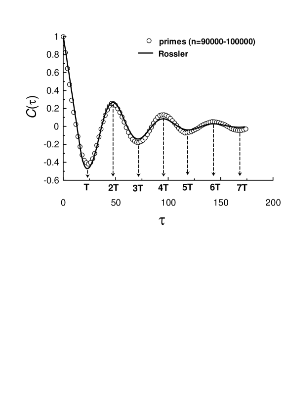
Figure 1: Autocorrelation of the $v(n)$ functions for the ln-sequence (circles) in the interval $9\times 10^{4}<n<10^{5}$. The solid line correspond to autocorrelation function computed for the telegraph signal generated by the Rössler attractor fluctuations overcoming the threshold $x=7$. In order to make the autocorrelation functions comparable a rescaling has been made for the Rössler autocorrelation function.

Let us consider a relatively short interval: $9\times 10^{4}<n<10^{5}$. For this interval the autocorrelation function

$$C(n,\tau)=\langle v(n)v(n+\tau)\rangle-\langle v(n)\rangle\langle v(n+\tau)\rangle$$

computed for the $v(n)$ function of the ln-sequence will be approximately independent on $n$. Figure 1 shows the autocorrelation function (circles) computed for the $v(n)$ function of the ln-sequence for the ’short interval’: $9\times 10^{4}<n<10^{5}$. Figure 2 shows an autocorrelation function (circles) computed for the $v(n)$ function of the ln-sequence for interval of much smaller natural numbers: $1000<n<2\times 10^{4}$ (here we rely on the much slower non-stationarity in the logarithmic gaps sequence in comparison with the original gaps sequence).

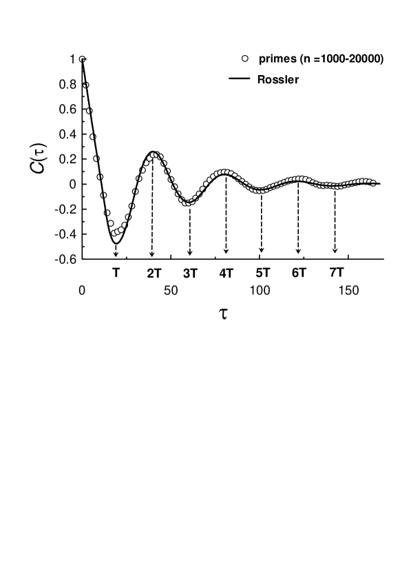
Figure 2: As in Fig. 1 but for interval $1000<n<2\times 10^{4}$.

3 Models

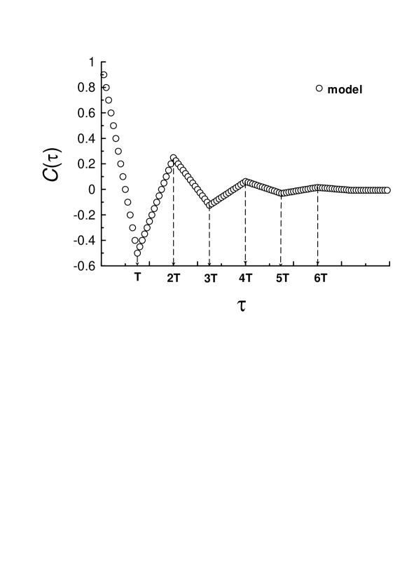
Figure 3: Autocorrelation function for the simple model telegraph signal: Eq. (3.2) with $q=0.25$.

In order to understand origin of the oscillating autocorrelation function shown in Figs. 1 and 2 let us consider a very simple telegraph signal, which allows analytic calculation of its autocorrelation function. The telegraph signal takes two values +1 or -1 and it changes its sign at discrete moments:

$$t_{n}=nT+\zeta$$

where $\zeta$ is an uniformly distributed over the interval $[0,T]$ random variable, $n=1,2,3...$ and $T$ is a fixed period. If $q$ is a probability of a sign change at a current moment ($0\leq q<1$), then the autocorrelation function of such telegraph signal is:

$$C(\tau)=(n-\tau/T)(2q-1)^{n-1}+(\tau/T-(n-1))(2q-1)^{n}$$

in the interval $(n-1)T\leq\tau<nT$. Figure 3 shows the autocorrelation function Eq. (3.2) calculated for $q=0.25$, as an example (cf. with Figs. 1 and 2). When parameter $q$ approaches value 0.5 the magnitude of the correlation function oscillations decreases . At value $q=0.5$ we have only linear decay in the interval $0\leq\tau<T$ and for $\tau\geq T$ the correlation function $C(\tau)=0$.

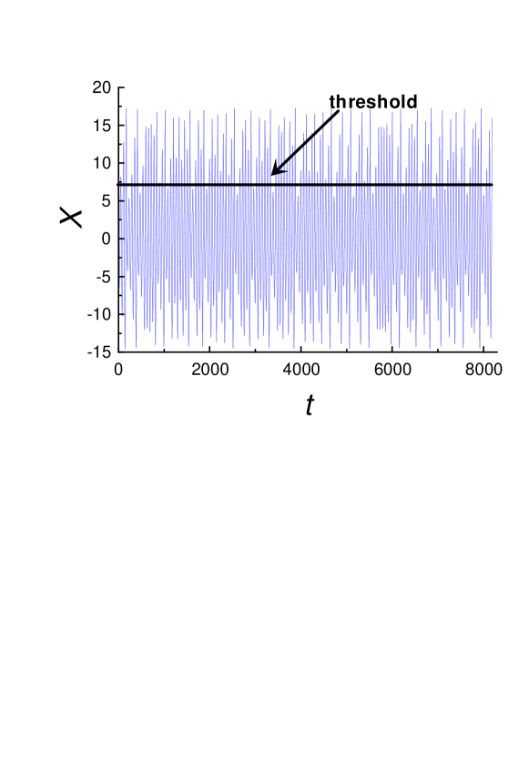
Figure 4: X-component fluctuations of a chaotic solution of the Rössler system Eq. (3.3) ($a=0.15,~{}b=0.20,~{}c=10.0$).

In the model Eq. (3.1) $\zeta$ was taken as a pure stochastic variable. This variable, however, can be also a chaotic (deterministic) one. Let us consider a chaotic solution of the Rössler system [9]

$$\frac{dx}{dt}=-(y+z);~{}~{}\frac{dy}{dt}=x+ay;~{}~{}\frac{dz}{dt}=b+xz-cz$$

where a, b and c are parameters (a reason for this system relevance will be given in Section 4). Figure 4 shows the x-component fluctuations of a chaotic solution of the Rössler system.

Let us consider a telegraph signal generated by the variable $x$ crossing certain threshold from below (Fig. 4). This telegraph signal takes values: +1 or -1, and changes its sign at the threshold-crossing points. Then, the fundamental period of the Rössler chaotic attractor provides the period $T$ in Eq. (3.1), whereas the chaotic fluctuations of the variable $x$ of the attractor provide chaotic variable $\zeta$ in the Eq. (3.1) for the considered telegraph signal. Autocorrelation function computed for this telegraph signal has been shown in Figs. 1 and 2 as the solid line. In order to make the autocorrelation functions comparable a rescaling has been made for the Rössler telegraph signal’s autocorrelation function.

Now, let us restore the fundamental period $T_{0}$ for the sequence of the first 10000 prime numbers:

$$T_{0}=\exp(T/10)\simeq 8\pm 1$$

where the period $T$ for the ln-sequence was taken from Figs. 1 and 2.

4 Twin prime killing method

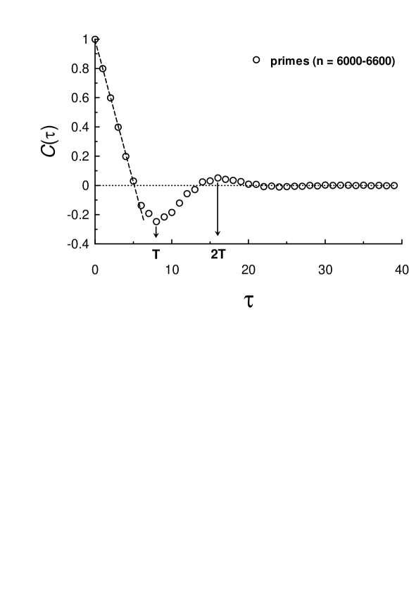
Figure 5: Autocorrelation of the $v(n)$ function for the K2-subsequence (circles) in the relatively short interval $6000<n<6600$.

One can expect that the smallest gaps between prime numbers are a source of the non-additive (high frequency) noise. Especially for small and moderate prime numbers where the minimal gap $\Delta=2$ occurs rather frequently. The primes separated by such gap are called twin primes. Let us kill one (say larger one) of the twin primes from each pair of the twin primes (a smart high frequency filter). Due to remaining part of the twins the subsequence of the primes preserves roughly the structure of the original full sequence of the primes (let us call this subsequence as K2-subsequence).

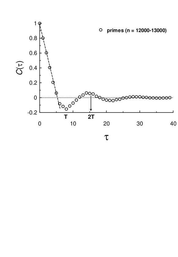
Figure 6: As in Fig. 5 but for interval $12000<n<13000$.

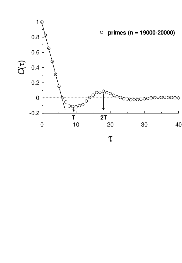
Figure 7: As in Fig. 5 but for interval $19000<n<20000$.

On the other hand, for small and moderate prime numbers the K2-subsequence can be expected to be less corrupted by the non-additive high frequency noise than the original sequence of the primes. Indeed, figure 5 shows autocorrelation of the $v(n)$ function for the K2-subsequence (circles) in the relatively short interval $6000<n<6600$. The dashed straight line indicates the characteristic linear decay (cf. with Figs. 1-3) and the arrows indicate the period $T=8\pm 1$. Figures 6 and 7 shows analogous results for the intervals $12000<n<13000$ and $19000<n<20000$ respectively. Comparing this result with Eq. (3.4) we can see good agreement between the values of the hidden period of the prime number sequence obtained by the two different methods: logarithmic gaps and twin prime killing.

It should be noted that the most probable value of the gap is $\Delta=6$ for the both original and K2-subsequence (one of the two integers nearest to any prime: $p-1$ or $p+1$, always has 6 as its divisor). Although the hidden period does not coincide with the most probable value of the gap (and apparently it is a subject of the prime number theorem), the simple 6-divisor could be a starting point in an attempt to understand origin of the hidden periodicity (in particular, the end-point of the linear decay in the Figs. 5-7 is always equal to 6, cf. with Fig. 3).

References

- [1] E. Bogomolny, Riemann zeta function and quantum chaos, Prog. Theor. Phys. Supplement, vol. 166, pp. 19-44, 2007.
- [2] K. Soundararajan, The distribution of prime numbers, NATO Science Series II: Mathematics, Physics and Chemistry, , vol. 237, pp. 59-83, 2007.
- [3] T. Timberlake and J.Tucker, Is there quantum chaos in the prime numbers?, Bulletin of the American Physical Society, vol. 52, p. 35, 2007, (arXiv:0708.2567).
- [4] C.E. Porter, Statistical Theories of Spectra: Fluctuations, NY: Academic Press, 1965.
- [5] M. Wolf, Applications of statistical mechanics in number theory, Physica A, vol. 274, pp. 149-157, 1999.
- [6] P. Kumar, P.Ch. Ivanov, and H.E. Stanley, Information Entropy and Correlations in Prime Numbers, arXiv:cond-mat/0303110.
- [7] S. Ares, and M. Castro, Hidden structure in the randomness of the prime number sequence?, Physica A, vol. 360, pp. 285-296, 2006.
- [8] S. R. Dahmen, S. D. Prado and T. Stuermer-Daitx, Similarity in the statistics of prime numbers, Physica A, vol. 296, pp. 523-528, 2001.
- [9] O.E. Rössler, An equation for continuous chaos, Phys. Lett. A, vol. 57, pp. 397-398, 1976.