Electronic structure via potential functional approximations

Abstract

The universal functional of Hohenberg-Kohn is given as a coupling-constant integral over the density as a functional of the potential. Conditions are derived under which potential-functional approximations are variational. Construction via this method and imposition of these conditions are shown to greatly improve the accuracy of the non-interacting kinetic energy needed for orbital-free Kohn-Sham calculations.

In the original form of density functional theory (DFT), suggested by ThomasT27 and FermiF28 (TF) and made formally exact by Hohenberg and KohnHK64 , the energy of a many-body quantum system is minimized directly as a functional of the density. Its modern incarnation uses the Kohn-Sham (KS) schemeKS65 , which employs the orbitals of a fictitious non-interacting system. This brilliant idea means only a small fraction of the total energy need be approximated, and good approximationsPBE96 ; Bb93 have made DFT the popular tool it is today. DFTFNM03 is now ubiquitous in many scientific fields, including both materials and chemistry.

Interest is rapidly reviving in finding an orbital-freeWC00 approach to DFT. The major bottleneck in modern calculations is the solution of the KS equations, which can be avoided with a pure density functional for the kinetic energy of non-interacting fermions, $T_{\scriptscriptstyle\rm S}$. The original TF approximation is of exactly this type, but is far too inaccurate for modern applications. Despite decades of effortDG90 , no generally applicable approximation for $T_{\scriptscriptstyle\rm S}$ has been found, although material-dependent approximationsHC10 have been suggested, or approximations designed only for weakly-interacting systemsW08 .

However, Englert and SchwingerES84 pointed out that the potential is a more natural variable to use in deriving approximations to quantum systems. In particular, semiclassical approximations begin with the classical momentum, a local functional of the potential. TF theory is often derived first in terms of the potential, which is then eliminated in the final expressions, yielding an explicit density functional. Exact potential functional theory (PFT) satisfies a variational principle with minimization over trial potentialsYAW04 ; GP09 , yielding useful insight into the optimized effective potential methodYAW04 .

In the present work we go beyond those results by considering explicit potential functional approximations to interacting and non-interacting systems of electrons; such approximations are presently being developed via a systematic asymptotic expansion in terms of the potential, which has already been found in simple casesELCB08 ; CLEB10 . The leading terms in a semiclassical expansion yield local approximations to the energies, and the leading corrections greatly improve over the accuracy of local approximations in a systematic and understandable way. Corrections to TF are relatively simple functionals of the potential, but far more subtle as functionals of the density. Such expansions are significantly more accurate and less problematic for the density itself rather than for the kinetic energy density because the latter requires two spatial derivativesCLEB10 .

By minimizing over $N$-particle wavefunctions $\Psi$ that are antisymmetric, normalized, and have finite kinetic energy, we obtain the ground-state (gs) energy

$$E_{v}=\min_{\Psi}\left(\langle\Psi\,|\ \hat{T}+\hat{V}_{\rm ee}+\hat{V}\ |\,\Psi\rangle\right)\,,$$ (1)

as a functional of the potential, where $\hat{T}$ is the kinetic energy operator, $\hat{V}_{\rm ee}$ the electron-electron repulsion, and $\hat{V}$ the one-body potential. We define the potential functionalYAW04 :

$$F[v]=\langle\Psi_{v}\,|\ \hat{T}+\hat{V}_{\rm ee}\ |\,\Psi_{v}\rangle,\,$$ (2)

with $\Psi_{v}$ denoting the gs wavefunction of potential $v({\bf r})$. With $F[v]$, the exact relation for the gs energy is

$$E_{v}=F[v]+\int d^{3}r\ n[v]({\bf r})\,v({\bf r})\,,$$ (3)

in practice, requiring approximations to both $F[v]$ and $n[v]$,

$$E^{\scriptscriptstyle\rm A,dir}_{v}=F^{\scriptscriptstyle\rm A}[v]+\int d^{3}r\ n^{\scriptscriptstyle\rm A}[v]({\bf r})\,v({\bf r})\,,$$ (4)

where $A$ denotes an approximation as a functional of the potential. We call this the direct approach.

We show that (i) the universal functional, $F[v]$, is determined entirely from knowledge of the density as a functional of the potential, such that only one approximation is required, namely $n^{\scriptscriptstyle\rm A}[v]$, (ii) the variational principle imposes a condition relating energy and density approximations, (iii) a simple condition guarantees satisfaction of the variational principle, (iv) with an orbital-free approximation to the non-interacting density as a functional of the potential, the kinetic energy is automatically determined, i.e., there is no need for a separate approximation, and (v) satisfaction of the variational principle improves accuracy of approximations.

We deduce an approximation to $F$ from any $n^{\scriptscriptstyle\rm A}[v]({\bf r})$ in the following way. Introduce a coupling constant in the one-body potential:

$$v^{\lambda}({\bf r})=(1-\lambda)\,v_{0}({\bf r})+\lambda\,v({\bf r})\,,$$ (5)

where $v_{0}({\bf r})$ is some reference potential (possibly $0$). In the context of TF theory this coupling was used in Ref. PHH88 . Then, using the Hellmann-Feynman theorem,

$$E_{v}=E_{0}+\int_{0}^{1}d\lambda\,\int d^{3}r\ n[v^{\lambda}]({\bf r})\,\Delta v({\bf r})\,,$$ (6)

where $\Delta v({\bf r})=v({\bf r})-v_{0}({\bf r})$. Defining $\bar{n}[v]({\bf r})=\int_{0}^{1}d\lambda\ n[v^{\lambda}]({\bf r})$ and choosing $v_{0}({\bf r})=0$, we obtain

$$F[v]=\int d^{3}r\left\{\bar{n}[v]({\bf r})-n[v]({\bf r})\right\}\;v({\bf r})\ .$$ (7)

This formula establishes that the universal functional is determined solely by the knowledge of the density as functional of the potential. Moreover, insertion of $n^{\scriptscriptstyle\rm A}({\bf r})$ on the right defines an associated approximate $F^{\rm cc}[n^{\scriptscriptstyle\rm A}[v]]$, where $cc$ denotes coupling constant.

On the other hand, much of the accuracy of DFT calculations derives from the variational principle. In PFT, this yields

$$E^{\scriptscriptstyle\rm A,var}_{v}=\min_{\tilde{v}}\left(F^{\scriptscriptstyle\rm A}[\tilde{v}]+\int d^{3}r\ n^{\scriptscriptstyle\rm A}[\tilde{v}]({\bf r})\,v({\bf r})\right),$$ (8)

with a possibly different value from Eq. (4) for a given pair of approximations. Experience suggests use of the variational principle improves results. The Euler equation for the minimum is

$$\frac{\delta F^{\scriptscriptstyle\rm A}[v]}{\delta v({\bf r})}=-\int d^{3}r^{\prime}\ v({\bf r}^{\prime})\,\chi^{\scriptscriptstyle\rm A}[v]({\bf r}^{\prime},{\bf r}),$$ (9)

where $\chi^{\scriptscriptstyle\rm A}[v]({\bf r},{\bf r}^{\prime})=\delta n^{\scriptscriptstyle\rm A}[v]({\bf r})/\delta v({\bf r}^{\prime})$ denotes the density-density response function. If a pair of approximations $\left\{F^{\scriptscriptstyle\rm A},n^{\scriptscriptstyle\rm A}\right\}$ satisfies Eq. (9) at $v({\bf r})$, then Eqs. (4) and (8) yield identical results, but this is not guaranteed a priori in approximate PFT.

We next ask: Does a given $F^{\rm cc}[n^{\scriptscriptstyle\rm A}[v]]$ satisfy Eq. (9)? Taking the functional derivative of Eq. (7) yields Eq. (9) if, and only if,

$$n^{\scriptscriptstyle\rm A}[v]({\bf r} )= \int_{0}^{1}d\lambda\int d^{3}r^{\prime}\ \Big{\{}\frac{\delta n^{\scriptscriptstyle\rm A}[v^{\lambda}[v]]({\bf r}^{\prime})}{\delta v({\bf r})}\,\frac{dv^{\lambda}[v]({\bf r}^{\prime})}{d\lambda}$$ (10)

$$+ n^{\scriptscriptstyle\rm A}[v^{\lambda}[v]]({\bf r}^{\prime})\,\frac{d}{d\lambda}\frac{\delta v^{\lambda}[v]({\bf r}^{\prime})}{\delta v({\bf r})}\Big{\}}.$$

This condition is true in turn, if and only if,

$$\chi^{\scriptscriptstyle\rm A}[v]({\bf r},{\bf r}^{\prime})=\chi^{\scriptscriptstyle\rm A}[v]({\bf r}^{\prime},{\bf r})\ .$$ (11)

The exact response function satisfies this relation, but an approximate functional $n_{\scriptscriptstyle\rm S}^{\scriptscriptstyle\rm A}[v]$ might not. This condition guarantees conservation of particle number under small changes in the potential, an elementary version of a conserving approximationBK61 .

A simple example illustrating these results is TF theory, considered as a potential functional. Then,

$$n^{\rm TF}[v]({\bf r})=\frac{1}{3\pi^{2}}\,\left[2(\mu-v_{\scriptscriptstyle\rm S}({\bf r}))\right]^{3/2}\,,$$ (12)

where $v_{\scriptscriptstyle\rm S}({\bf r})=v({\bf r})+v_{\scriptscriptstyle\rm H}({\bf r})$, and the latter is the Hartree potential, determined self-consistently from

$$\nabla^{2}v_{\scriptscriptstyle\rm H}({\bf r})=-4\pi\,n^{\rm TF}({\bf r})\,,$$ (13)

while $\mu$ is the chemical potential, determined by the normalization requirement that $\int d^{3}r\ n({\bf r})=N$. Taking functional derivatives with fixed $N$, the usual TF energy expressionCB11

$$F^{\rm TF}[v]=T_{\scriptscriptstyle\rm S}^{\rm TF}[v]+\int d^{3}r\,n^{\rm TF}[v]({\bf r})\ v({\bf r})+U[n^{\rm TF}[v]]$$ (14)

satisfies the Euler condition when combined with Eq. (12), and $F^{\rm cc}[n^{\rm TF}[v]]=F^{\rm TF}[v]$, where $T_{\scriptscriptstyle\rm S}^{\rm TF}[v]=\pi^{2}\int d^{3}r\ n^{\rm TF}[v]({\bf r})^{3}/6$ denotes the TF kinetic energy and $U[n^{\rm TF}[v]]=\int d^{3}r\ n^{\rm TF}[v]({\bf r})\ v_{\scriptscriptstyle\rm H}[n^{\rm TF}[v]]({\bf r})/2$ the Hartree energy.

In practice, the usefulness of these results for interacting electrons might be limited, as they require an approximation to the interacting density as a functional of the one-body potential that is sufficiently accurate to be competitive with standard KS-DFT calculations, i.e., beyond the accuracy of TF theory. Of much more practical use is their application to the non-interacting electrons of the KS scheme, which sit in the effective KS potential, which includes both a Hartree and (some approximate) exchange-correlation (XC) contribution:

$$v_{\scriptscriptstyle\rm S}({\bf r})=v({\bf r})+\int{\mathrm{d}}^{3}r^{\prime}\ \frac{n^{\scriptscriptstyle\rm A}_{\scriptscriptstyle\rm S}[v_{\scriptscriptstyle\rm S}]({\bf r}^{\prime})}{|{\bf r}-{\bf r}^{\prime}|}+v_{\scriptscriptstyle\rm XC}^{\scriptscriptstyle\rm A}[n^{\scriptscriptstyle\rm A}_{\scriptscriptstyle\rm S}[v_{\scriptscriptstyle\rm S}]]({\bf r})\,.$$ (15)

For a given approximation to $E_{\scriptscriptstyle\rm XC}$, which determines $v^{\scriptscriptstyle\rm A}_{\scriptscriptstyle\rm XC}$, this equation can be easily solved by standard iteration techniques, bypassing the need to solve the KS equations. A given $n_{\scriptscriptstyle\rm S}^{\scriptscriptstyle\rm A}[v_{\scriptscriptstyle\rm S}]$ removes the need for solving any differential equation in each iteration.

However, once self-consistency is achieved, we need to extract the total energy of the interacting electronic system, for which we need the kinetic energy of the KS electrons. All our derivations apply equally to the non-interacting problem, so we deduce:

$$T_{\scriptscriptstyle\rm S}[v]=\int d^{3}r\left\{\bar{n}_{\scriptscriptstyle\rm S}[v]({\bf r})-n_{\scriptscriptstyle\rm S}[v]({\bf r})\right\}\;v({\bf r})\,,$$ (16)

which is the analog of Eq. (7) for a system of non-interacting electrons in the external potential $v({\bf r})$ (which is called $v_{s}(r)$, when it is the KS potential of some interacting system). This defines a kinetic energy approximation determined solely by the density approximation:

$$T_{\scriptscriptstyle\rm S}^{\rm cc}[n_{\scriptscriptstyle\rm S}^{\scriptscriptstyle\rm A}[v]]=\int d^{3}r\left\{\bar{n}_{\scriptscriptstyle\rm S}^{\scriptscriptstyle\rm A}[v]({\bf r})-n_{\scriptscriptstyle\rm S}^{\scriptscriptstyle\rm A}[v]({\bf r})\right\}\,v({\bf r})\ .$$ (17)

This is our main result for the non-interacting case. It eliminates the need for constructing approximations to the non-interacting kinetic energy $T_{\scriptscriptstyle\rm S}$.

To illustrate the power of these results, we consider a simple example, a system of non-interacting, spinless fermions in a one-dimensional box. We choose $v_{0}(x)$ to be $0$ inside a box ($0<x<L$), and $\infty$ outside. Then $\Delta v(x)=v(x)$ is some potential inside the box. For this case Eq. (17) (with a nonzero $v_{0}$) reduces to

$$T_{\scriptscriptstyle\rm S}^{\rm cc}[n_{\scriptscriptstyle\rm S}^{\scriptscriptstyle\rm A}[v]]=E_{0}(N)+\!\int_{0}^{L}\!\!\!\!\!dx\left\{\bar{n}_{\scriptscriptstyle\rm S}^{\scriptscriptstyle\rm A}[v](x)-n_{\scriptscriptstyle\rm S}^{\scriptscriptstyle\rm A}[v](x)\right\}v(x)\,,$$ (18)

where $E_{0}(N)=\pi^{2}\,\left(N^{3}+3/2\,N^{2}+N/2\right)/6$ denotes the total non-interacting energy of $N$ spinless fermions in an infinite square well.

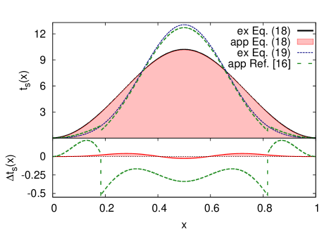
Figure 1: Exact (ex) and approximate (app) kinetic energy densities (above) of Eq. (18) (black, red) and of Eq. (19) (blue, green) with the approximation in Ref. CLEB10 , and their absolute errors (below) for one particle in $v(x)=-5\,\sin^{2}(\pi x)$, $0~{}<~{}x~{}<~{}1$. (color online)

In Fig. 1 we plot two distinct kinetic energy densities, along with approximations to them, and the corresponding errors, for $v(x)=-5\sin^{2}(\pi x)$ in a box of unit length. The blue curve is the exact kinetic energy density obtained from a traditional definition,

$$t_{\scriptscriptstyle\rm S}(x)=-\frac{1}{2}\sum_{j=1}^{N}\phi_{j}^{*}(x)\frac{\partial^{2}}{\partial x^{2}}\phi_{j}(x)\,,$$ (19)

while the green curve is the approximation derived at great length in Ref. CLEB10 . The small discontinuity at about $x=0.2$ and $0.8$ is where the approximation switches from a form that is asymptotically correct in the interior to one that is asymptotically correct near the walls. The error is shown in the bottom panel. Note that the approximation for $t_{\scriptscriptstyle\rm S}(x)$ of Ref. CLEB10 is already a considerable improvement over that used in Ref. ELCB08 . The red and black curves result from Eq. (18). The black is exact, while the red uses the approximation for the density in Ref. ELCB08 . Their difference is plotted in the bottom panel, and is both locally and globally far smaller, and required no separate approximation for the kinetic energy density.

The approximations of Refs. ELCB08 and CLEB10 were designed to be asymptotically exact as $N\to\infty$, both for the density and the kinetic energy. In Table 1 we show errors compared to the exact result of $T_{\scriptscriptstyle\rm S}^{\scriptscriptstyle\rm A}$ from TF theory, the WKB approximation, Ref. ELCB08 , its improvement in Ref. CLEB10 , and $T_{\scriptscriptstyle\rm S}^{\rm cc}$ in Eq. (18) with $n_{\scriptscriptstyle\rm S}^{\scriptscriptstyle\rm A}[v]$ of Ref. ELCB08 .

Table 1: Total non-interacting kinetic energy of N particles and its absolute error in TF, WKB, $T_{\scriptscriptstyle\rm S}^{\scriptscriptstyle\rm A}$ of Ref. ELCB08 and CLEB10 , and $T_{\scriptscriptstyle\rm S}^{\rm cc}$ of Eq. (18) for the potential of Fig. 1.

		$|T_{\scriptscriptstyle\rm S}-T_{\scriptscriptstyle\rm S}^{\scriptscriptstyle\rm A}|$
$N$	$T_{\scriptscriptstyle\rm S}$	TF	WKB	Ref. ELCB08	Ref. CLEB10	$T_{\scriptscriptstyle\rm S}^{\rm cc}$
1	4.97	3.16	1.42	0.47	0.12	$1.2\cdot 10^{-2}$
2	24.73	11.50	1.47	0.43	0.08	$2.0\cdot 10^{-3}$
4	148.08	42.76	1.48	0.50	0.04	$4.0\cdot 10^{-4}$

Even for $N=1$, $T_{\scriptscriptstyle\rm S}^{\rm cc}$ is about two orders of magnitude more accurate than WKB, and significantly more accurate than the direct approximations of Refs. ELCB08 and CLEB10 . As $N\to\infty$, $T_{\scriptscriptstyle\rm S}^{\rm cc}$ converges most rapidly.

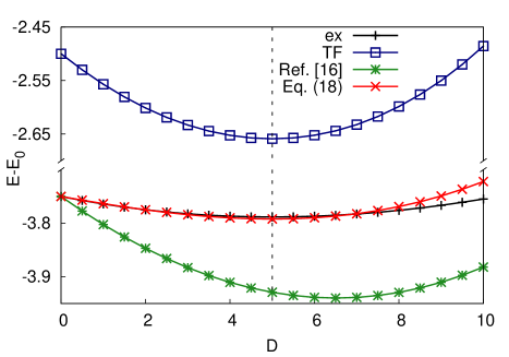
Figure 2: Difference of total exact (ex) energy $E$ and $E_{0}$ (black) compared to the TF approximation (blue), $T_{\scriptscriptstyle\rm S}^{\scriptscriptstyle\rm A}$ of Ref. CLEB10 (green) and $T_{\scriptscriptstyle\rm S}^{\rm cc}$ of Eq. (18) (red) for $N=1$ and trial potentials $\Delta\tilde{v}(x)=-D\sin^{2}(\pi x)$. (color online)

We finally test the symmetry condition of Eq. (11). To do this, we perform a variational PFT calculation, implementing Eq. (18). We take a given external potential ($-5\sin^{2}(\pi x)$), calculate exact gs wave functions with different potentials, and find their energy. Fig. 2 shows the results when the well depth $D$ is varied. The exact result is a black curve, whose minimum occurs at $D=5$. The blue curve is the result of TF theory, which satisfies the condition, but is not very accurate. The green curve is the approximation of Ref. CLEB10 , which, while more accurate, does not minimize at the true potential. This demonstrates that the pair of approximations $T_{\scriptscriptstyle\rm S}^{\scriptscriptstyle\rm A}[v]$ and $n_{\scriptscriptstyle\rm S}^{\scriptscriptstyle\rm A}[v]$ given there do not yield the same answer variationally and directly. Note also that the direct evaluation (green curve at $D=5$) is more accurate, when compared to the exact result (black curve at $D=5$) than application of the variational principle (green curve at its mininum $D\approx 6.5$). This is because these approximations were derived semiclassically, and have uncontrolled errors. On the other hand, our coupling-constant approximation of Eq. (18) (red curve) is both far more accurate and minimizes at the true potential.

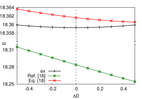
Figure 3: Exact (ex) total energy (black) compared to the direct approximation of Ref. CLEB10 (green) and $T_{\scriptscriptstyle\rm S}^{\rm cc}$ of Eq. (18) (red) for $N=2$ and trial potentials $\tilde{v}(x)=-5\sin^{2}(\pi x)-\Delta D\sin^{2}(2\pi x)$ with the external potential at $\Delta D=0$. (color online)

However, we further tested the coupling-constant approximation by adding the perturbation $-\Delta D\sin^{2}(2\pi x)$ with varying depth $\Delta D$ to the given external potential ($-5\sin^{2}(\pi x)$). For $N=2$, as shown in Fig. 3, the minimum is no longer at $\Delta D=0$, despite the high accuracy. This demonstrates that Eq. (11) is not satisfied for all possible variations of the potential around the true one. However, the breakdown appears small and does not much diminish accuracy. This breakdown is due to the small normalization error in the semiclassical densityCLEB10 . If the error changes with the potential, the corresponding $\chi^{A}$ cannot be symmetric. We have also calculated the response function for that approximation and found non-symmetrical termsCB11 . This shows the utility of our analysis: Accuracy is likely to be further improved if the result can be easily modified to enforce Eq. (11).

An alternative to the coupling-constant method used here is the virial theorem, which yields the kinetic energy from the potential and density aloneMY59 . We recommend that version which has an origin-independent kinetic energy density given in Ref. SLBB03 , satisfying

$$\nabla^{2}t_{\scriptscriptstyle\rm S}({\bf r})=-\frac{d}{2}\nabla\{n({\bf r})\,\nabla v_{\scriptscriptstyle\rm S}({\bf r})\}\,,$$ (20)

where $d$ denotes the dimension of space. While either the virial or the coupling-constant formulation can be applied to realistic systems, we use the coupling constant here because our illustrations involve box-boundary conditions, which create complications for the virial theoremCP51 .

The coupling-constant formulation can be applied to realistic systems with potentials that vanish at large distances, using $v_{0}=0$ for a reference. Then, to keep the particle number fixed, employ the device of putting the system in a large box whose size is taken to $\infty$ at the end of the calculation. Either expression has a great advantage over traditional density-functional approximations, such as generalized gradient approximations. For such approximations, there is always an ambiguity in the energy densities; a term that integrates to zero over the entire space can always be addedPSTS08 . However our energies use an approximation to the density, which is uniquely determined for all ${\bf r}$, and so can be used to identify the relative contribution to the energy from different regionsCB11 .

Which variation (coupling constant or virial) is most useful in practice awaits general-purpose approximations for the density as a functional of the potential for an arbitrary three-dimensional case. But at least it no longer awaits the corresponding kinetic energy approximations.

We gratefully acknowledge funding from NSF under grant number CHE-0809859.

References

- (1) L. H. Thomas, Math. Proc. Camb. Phil. Soc. 23, 542 (1927).
- (2) E. Fermi, Z. Phys. 48, 73 (1928).
- (3) P. Hohenberg and W. Kohn, Phys. Rev. 136, B864 (1964).
- (4) W. Kohn and L. J. Sham, Phys. Rev. 140, A1133 (1965).
- (5) J. P. Perdew, K. Burke, and M. Ernzerhof, Phys. Rev. Lett. 77, 3865 (1996).
- (6) A. D. Becke, J. Chem. Phys. 98, 5648 (1993).
- (7) C. Fiolhais, F. Nogueira, and M. Marques, editors, A Primer in Density Functional Theory, Springer-Verlag, NY, 2003.
- (8) Y. A. Wang and E. A. Carter, Orbital-free kinetic-energy density functional theory, in Theoretical Methods in Condensed Phase Chemistry, edited by S. D. Schwartz, chapter 5, page 117, Kluwer, Dordrecht, 2000.
- (9) R. M. Dreizler and E. K. U. Gross, Density Functional Theory: An Approach to the Quantum Many-Body Problem, Springer–Verlag, 1990.
- (10) C. Huang and E. A. Carter, Phys. Rev. B 81, 045206 (2010).
- (11) T. A. Wesolowski, Phys. Rev. A77, 012504 (2008).
- (12) B.-G. Englert and J. Schwinger, Phys. Rev. A 29, 2339 (1984).
- (13) W. Yang, P. W. Ayers, and Q. Wu, Phys. Rev. Lett. 92, 146404 (2004).
- (14) E. K. U. Gross and C. R. Proetto, J. Chem. Theory Comput. 5, 844 (2009).
- (15) P. Elliott, D. Lee, A. Cangi, and K. Burke, Phys. Rev. Lett. 100, 256406 (2008).
- (16) A. Cangi, D. Lee, P. Elliott, and K. Burke, Phys. Rev. B 81, 235128 (2010).
- (17) L. R. Pratt, G. G. Hoffman, and R. A. Harris, J. Chem. Phys. 88, 1818 (1988).
- (18) G. Baym and L. P. Kadanoff, Phys. Rev. 124, 287 (1961).
- (19) A. Cangi and K. Burke, long paper in prep (2011).
- (20) N. H. March and W. H. Young, Nucl. Phys. 12, 237 (1959).
- (21) E. Sim, J. Larkin, K. Burke, and C. Bock, J. Chem. Phys. 118, 8140 (2003).
- (22) T. Cottrell and S. Paterson, Phil. Mag. 42, 391 (1951).
- (23) J. P. Perdew, V. N. Staroverov, J. Tao, and G. E. Scuseria, Phys. Rev. A 78, 052513 (2008).