Abstract:

We study a simple general scenario of ad hoc networks based on IEEE 802.11 wireless communications, consisting in a chain of transmitters, each of them being in the carrier sense area of its neighbors. Each transmitter always attempts to send some data frames to one receiver in its transmission area, forming a pair sender-receiver. This scenario includes the three pairs fairness problem introduced in [1], and allows to study some fairness issues of the IEEE 802.11 medium access mechanism.

We show by simulation that interesting phenomena appear, depending on the number $n$ of pairs in the chain and of its parity. We also point out a notable asymptotic behavior. We introduce a powerful modeling, by simply considering the probability for a transmitter to send data while its neighbors are waiting. This model leads to a non-linear system of equations, which matches very well the simulations, and which allows to study both small and very large chains. We then analyze the fairness issue in the chain regarding some parameters, as well as the asymptotic behavior. By studying very long chains, we notice good asymptotic fairness of the IEEE 802.11 medium sharing mechanism. As an application, we show how to increase the fairness in a chain of three pairs.

 

1 Introduction

1.1 Motivations

Recently, wireless networks have increasingly received attention from the networking community. Although several wireless communication standards have been proposed, the IEEE 802.11 protocol [2, 3, 4] is the most widely used, and constitutes the de facto solution for practical network connection offering mobility, flexibility, low cost of deployment and use. This success leads to many studies of the protocol, in various situations (either ad hoc or with access point) and by different means (experimentation, simulation, modeling). It remains that, besides its qualities, the 802.11 protocol, and particularly its medium access control mechanism, suffers from some imperfections in terms of global throughput and fairness between nodes. Our work deals with some fairness issues with 802.11 protocol in ad hoc mode.

We study a simple but general scenario, where some nodes (hereby called senders) try to continuously send some data to one of their neighbors (hereby called receiver), not necessarily always the same. The senders form a chain, each of which being in the carrier sense area of its neighbors (Figure 1).

Figure 1: A chain of senders.

In [1], the authors study a similar scenario composed of three pairs, and shows that the central pair obtains a very poor throughput compared to the border pairs. For instance, with a sending rate of 2 Mbits/s, the central pair has only a throughput of 0.04 Mbits/s compared to 1.55 Mbits/s for the external ones (the throughput of a single alone pair is 1.59 Mbits/s in this situation).

This scenario is a particular case of the chain of senders scenario we study in this paper. It combines both EIFS delay mechanism and asymmetry of the chain in terms of number of neighbor senders. We show that interesting phenomena appear when the number of pairs increases in the chain. These phenomena depend on the number $n$ of pairs as well as on its parity. Moreover a notable asymptotic behavior appears when $n$ increases. We provide a powerful modeling which leads, among others, to interesting conclusions in terms of fairness both for small and large chains. This analysis allows us to better understand the DCF properties and to improve the fairness in a chain, especially in the three pairs case.

1.2 Related work

There is a large amount of literature dealing with the performances of the IEEE 802.11 Distributed Coordinated Function (DCF) responsible of the shared radio medium sharing.

In [5], a relation between the necessary and real time for sending some data is given, allowing to estimate the DCF capacity. In [6] the authors make an analytical study of the rates calculation of the DCF using Markov chain. The authors prove that the performances of the DCF depends on the minimal contention window and on the number of stations in the network.

In [7], a modeling of the IEEE 802.11 DCF with stochastic Petri nets is proposed. Among other results, the authors show that the EIFS delay used when a collision occurs can be advantageous when the network is not saturated.

In [8], the authors modify the model suggested in [6], and give an estimation of the throughput as a function of the number of stations in the network and of the ambient noise. Reusing works of [6, 5], the authors improve their results in [9], by taking into account the contention window increasing in case of collision.

Besides throughput evaluation, some studies deal with the DCF fairness.

In [10], the authors present a case where the binary exponential backoff (BEB) lead to an unfair situation. Indeed, consider a situation where the contention window of the competing transmitters are large due to collisions. As soon as a node succeeds in sending a frame, it will reset its contention window. As a consequence, it will generally wait for smaller backoff than others for its further transmissions, and then gain more easily access to the shared medium. To resolve such problems, the authors design the medium access protocol MACAW.

In [11], the authors present the relevance of the EIFS mechanism to the fairness. They show that the EIFS delay can be too large or too small according to some scenarios. The authors propose then an adaptive mechanism for determining the EIFS delay, based on a measurement of the occupation time of the medium.

In [12] the authors propose an evaluation of the DCF fairness, by means of maximization of some differentiable concave functions, under a set of constraints representing the impossibility for two close transmitters to simultaneously transmit a frame with success. Some unfair situations relying on asymmetric topologies are studied by simulation. They also study fairness per packets and fairness per flow: two mobiles with the same probability of access to the medium do not constitute an equitable scenario when one of both must retransmit more flow than the other.

In [1, 13], the authors study an unfair scenario called three pairs problem by means of simulations and experimentations. This scenario relies on an asymmetric topology composed of three pairs of nodes. Pair 2 is placed between pairs 1 and 3, and is in the carrier sense of its both neighbors. The emissions of pairs 1 and 3 are not synchronized, and when the pair 2 wants to emit, it is necessary that the silence periods of the other mobiles overlap. However the probability of such a covering is weak.

This scenario has been modeled in [14] with a discrete time Markov chain. The authors obtain results close to the simulations.

1.3 Contributions and outlines

In Section 2, we summarize the main characteristics of the IEEE 802.11 standard when used in ad hoc networks with 802.11b devices. We then present in Section 3 our chain of senders scenario. Numerical values are given assuming a Lucent Orinoco 802.11b wireless device. Comments of the three pairs fairness problem introduced in [1] are also given.

In Section 4, we show by simulation using Network Simulator, that interesting phenomena appear when varying the number $n$ of pairs: i) chance to gain access to the medium for the $i$th sender-receiver pair depends on the parity of $i$, ii) the fairness increases with $n$ especially for central pairs and iii) the system has an asymptotic behavior when $n$ increases.

In Section 5, we introduce a new modeling of such a phenomenon. Although it is quite simple, it allows to match results of simulations both for small and large values of $n$, depending on a $\alpha$ coefficient. This coefficient corresponds to the probability of emission when the neighbor senders are waiting. For small values of $n$, we give close expressions (depending on $\alpha$) for the probability of emission of a given pair.

In Section 6, we prove that a stationary state exists for each pair for any length of the chain. Moreover, this stationary state converge to an asymptotic stationary state when $n$ increases. This confirms the simulations. We also show that some values of $\alpha$ allows to maximize the fairness, expressed as entropy [15].

In Section 7, we comment these results, and we show that when $n$ is large, the fairness is almost optimal near the center of the chain. We also show that the simulation results tend to this ideal case when $n$ increases. Finally, we sketch the relationship between $\alpha$ and the IEEE 802.11 protocol, and we explain how to optimize the fairness by means of packet size tuning relying on $n$ and $\alpha$. As an application of our analytical study, we maximize the fairness in the three pairs scenario.

Concluding remarks end the paper.

2 IEEE 802.11 standard in ad hoc mode

The IEEE 802.11 standard implements several types of wireless communications [2]. We focus on the most widely used for ad hoc networking with 802.11b compliant devices in order to explain the numerical values of this paper. We first begin by the physical layer and then we summarize the medium access layer. Note that the numerical values depend on the physical layer we describe, but this is not the case for the fairness issues we point out, which appears also in protocols based on other physical layer (such 802.11a or 802.11g for instance).

2.1 Physical layer

In the 802.11 standard, the physical layer (PHY) is divided into two sublayers: the Physical Medium Dependent (PMD) covered by the Physical Layer Convergence Sublayer.

2.1.1 PMD sublayer

Besides the infra-red communications, the 802.11 PMD has been declined into two physical layers for radio-communications, based on spread spectrum: FHSS and DSSS. The spread spectrum techniques uses a wider bandwidth than needed for sending a message, leading to low power density and redundancy: less energy is diffused on a given frequency causing less interferences with the environment, and a given information is present in several frequencies ensuring better noise robustness. Others physical layers have been introduced in some addenda: HR-DSSS in [3] and OFDM in [4]. With the Channel Agility option, a PMD can switch from one modulation to another. However, ad hoc networks based on the IEEE 802.11b standard mainly rely on the DSSS and HR-DSSS PMD layers, operating in the 2.4-2.485 GHz frequency range included into the Industrial, Scientific and Medical (ISM) frequencies. We know summarize these modulations.

For the Direct Sequence Spread Spectrum (DSSS), the 2.4 GHz ISM range is divided into 14 channels of 22 MHz each, with partial overlapping. A single frequency is used for transmission. However a chipping technique adds redundancy to increase the robustness: each bit of data is coded by a sequence of eleven chips using a Barker code. The modulation technique is the Differential Binary (resp. Quadrature) Phase Shift Keying (DBPSK, resp. DQPSK) which offers a sending rate of 1 Mbits/s for the DBPSK and 2 Mbits/s for the DQPSK. In these techniques, a phase rotation is performed depending on the symbol to send (either one bit for DBPSK or two for DQPSK). These modulation techniques admit a better minimum signal to noise ratio of about 12 dB than FHSS. However the transmission is more sensitive to multi-paths, and to Bluetooth emissions (which uses the same bandwidth range).

The High Rate DSSS (HR-DSSS) uses a more complex modulation technique called Complementary Code Keying (CCK). A sending rate of 5.5 Mbits/s (resp. 11 Mbits/s) is reached with four (resp. eight) symbols per chips. The different sending rates are chosen dynamically on the basis of transmission conditions, for instance the signal to noise ratio (this is not normalized). In practice, in outdoor environment, the 11Mbits/s is admissible until about 200 m, the 5.5 Mbits/s until about 300 m, the 2 Mbits/s until 400 m and the 1 Mbits/s until 500 m. This of course depends on the devices (power), antenna (gain) and environment (outdoor/indoor, obstacles, noise…).

2.1.2 PLCP sublayer

This sublayer makes a link between the different PMD layers and the MAC layer (which should not depend on the physical layer, either current or future). It prepares the MAC formated packets for the relevant PMD layer. A header and a preamble are inserted before any sent data in order to synchronize the sender and the receiver, to choose the modulation technique, and so on. As explained above, several data rates are available in the IEEE 802.11b standard based on DSSS modulations: 1 Mbits/s, 2 Mbits/s, 5.5 Mbits/s and 11 Mbits/s. While the norm admits the optional short preamble and header option (120 bits partially sent at 2 Mbits/s requiring 96 $\mu$s), both preamble and header are generally sent at the low sending rate (1Mbits/s using the DBPSK modulation) in order to be understood by every stations (long preamble and header default option).

The (long) PLCP preamble is composed of 128 bits used for sender and receiver auto-synchronization (SYNC field) and 16 bits for the Start Field Delimiter (SFD), that indicates the beginning of the frame. This corresponds to 144 $\mu$s. The (long) PLCP header is composed of the SIGNAL field (8 bits) to indicate the modulation technique which is used (either DBPSK or DQPSK), the SERVICES field (8 bits, currently unused), the LENGTH field (16 bits) to indicate the number of microseconds required for transmitting the data of the MAC layer, and the CRC field (16 bits) used for the cyclic redundancy code checking. This corresponds to 48 $\mu$s. PLCP preamble and header lead to a total of 192 $\mu$s at the beginning of any sending.

The PLCD sublayer also implements the Carrier Sense/Clear Channel Assessment (CS/CCA) procedure, which gives informations on the medium (either idle or busy). It is used to detect the beginning of a network signal which can be received (CS), and to determine whether the channel is clear prior to transmit a packet (CCA). The duration of this procedure depends on the modulation technique: 27 $\mu$s for FHSS, less than 15 $\mu$s for DSSS and HR-DSSS. It impacts the value of the aSlotTime constant used by the MAC layer. By adding other PHY-dependent delays, we found a slot time of 50 $\mu$s for the FHSS and 20 $\mu$s for the DSSS and HR-DSSS modulations.

2.2 Medium Access Control layer

The purpose of the MAC layer is to control the access to the shared medium by the neighborhood nodes. Two methods have been defined: the Distributed Coordination Function (DCF) and the Point Coordination Function (PCF). The fundamental access method is the DCF; the PCF is optional. We focus on the DCF method which is the only used in practice (PCF is rarely implemented). We first describe frames to explain durations used in the rest of the paper.

2.2.1 Frames

A MAC frame is composed of a MAC header (10 to 30 bytes, depending on the kind of frame), a body (0 to 2312 bytes) and a Frame Check Sequence (FCS, 4 bytes). The MAC header contains at least a Frame Control field (2 bytes), a Duration field (2 bytes) and a MAC address (6 bytes) leading to a minimum frame size of 14 bytes with the FCS field and an empty body. The header of a frame sent from one mobile to another one in an ad hoc network is 24 bytes width.

Any frame is acknowledged by the receiver (unicast), implementing a positive acknowledgment. If the acknowledgment has not been received before a delay ACK_TIMEOUT, the frame is sent again. An acknowledgment is a 14 bytes length MAC frame (needing 304 $\mu$s at 1 Mbits/s when adding the PLCP header and preamble).

2.2.2 Delays

The DCF implements a Carrier Sense Multiple Access protocol with Collision Avoidance (CSMA/CA). It is designed to reduce the collision probability by inserting some delays between contiguous frames (interframe spaces, IFS). The duration of the delay depends on the situation. Any transmission should begin by a DCF IFS (DIFS) delay. The acknowledgment is sent by the receiver after a Short IFS (SIFS). The SIFS is smaller than the DIFS to give priority to the acknowledgement to other transmissions.

If a station $S_{2}$ receives a frame but is not able to understand it (erroneous frame), it waits during an Extended IFS (EIFS) instead of a DIFS before sending. This could be a frame sent by $S_{1}$ to $R_{1}$, and these stations are too far from $S_{2}$ to allow a good reception by this station (preamble and header are sent using the DBPSK modulation at 1 Mbits/s, and can be understood while the rest of the frame sent at higher rate with a different modulation could not be understood). The EIFS delay allows to $R_{1}$ to acknowledge the frame sent by $S_{1}$. This prevents some cases when $S_{2}$ does not hear the acknowledgment sent by $R_{1}$, and begins a transmission that could prevent the acknowledgment reception on $S_{1}$. The station $S_{2}$ will switch from EIFS to DIFS delays after receiving a correct frame.

As for the aSlotTime constant, the duration of the SIFS delay depends on the PHY layer. It is equal to 10 $\mu$s for DSSS and HR-DSSS. The DIFS delay is equal to a SIFS delay plus two aSlotTime, leading to 50 $\mu$s for DSSS and HR-DSSS. The EIFS delay is equal to a SIFS delay plus the duration of an acknowledgment (sent at the lowest sending rate of 1 Mbits/s) plus the duration of a preamble and a header of the PLCP sublayer plus a DIFS delay, leading to 364 $\mu$s for DSSS and HR-DSSS.

2.2.3 RTS/CTS

Both physical and virtual mechanisms are available to sense the carrier. As already seen, the PLCP sublayer provides a CS/CCA function which is used by the MAC layer to probe the channel. Moreover, each station maintains a Network Allocation Vector (NAV) in order to foresee the channel liberation. The NAV is updated using the duration field included in the received frames. A station cannot attempt to transmit if its NAV indicates that the medium is busy. However a station $S_{2}$ which is not in the neighborhood of the sender $S_{1}$ but is in the neighborhood of the receiver $R_{1}$ could begin to send data during the current transmission from $S_{1}$ to $R_{1}$, leading to a congestion on $R_{1}$. To avoid this problem (hidden station), the sender $S_{1}$ can first send a Request To Send (RTS) message to $R_{1}$, which will then reply by a Clear To Send (CTS). The station $S_{2}$ will receive the CTS message, and will then update its NAV, preventing it to send data during the transmission $S_{1}\rightarrow R_{1}$. The frames RTS and CTS are followed by a SIFS delay.

A RTS frame has the same length than an ACK frame (14 bytes, 304 $\mu$s at 1 Mbits/s). A CTS frame is 20 bytes long (352 $\mu$s at 1 Mbits/s) because the header contains an additional MAC addresses. These frames are supposed to be shorter than the data frames, and then less subject to collisions. Depending on the configuration, this mechanism is i) never used, ii) always used or iii) used when the frame length is larger than a threshold.

2.2.4 Backoff

Despite the inter-frames delays and the carrier sense before any transmission, several stations could decide to send simultaneously as soon as the medium is clear. To minimize such a situation, any station waits for a random delay called backoff time before beginning a transmission.

After the DIFS or EIFS delay has expired, and if no current backoff time remains, the station generates a random number $x$ between $0$ and the value of a Contention Window (CW). The backoff time is then equal to $x\times$aSlotTime. Each time the channel is idle during aSlotTime microseconds, the backoff time is decreased of aSlotTime microseconds. The backoff time does not decrease if the medium is busy. The transmission can begin if the channel is idle and both the delay (either DIFS or EIFS) and the backoff time has been expired.

The value of the contention window belongs to the interval CWmin and CWmax, where CWmin depends on the physical layer (31 for DSSS and HR-DSSS) and CWmax equals to 1023. At the beginning, CW is equal to CWmin. Every time an attempt to transmit fails, the contention window is doubled ($\mbox{CW}\leftarrow\mbox{CW}\times 2+1$) until it reaches CWmax. The contention window is reset to CWmin after a successful transmission (or after a fixed number of attempts). A successful transmission includes an acknowledged frame as well as the receiving of a CTS frame in response to a RTS frame.

3 Fairness issues in a chain of senders

The DCF mechanism described in the previous section ensures a fair access to the shared medium when the competing nodes are able to hear each of them. However in more complexe multi-hop ad hoc networks, some cases of unfairness could be caused by asymmetry of the topology, or by the use of the EIFS delay by some nodes while others use the DIFS [12, 13]. In this section, we present an unfair case which appears in a chain of senders. This is a more general case than the already known three pair problem introduced in [1]. We begin by some considerations on distances between mobiles.

3.1 Transmission ranges considerations

In the 802.11 standard, the PHY layer reports the reception of a message only if the Signal to Noise Ratio (SNR) is larger than a fixed threshold (SNR_THRESHOLD). A signal sent with a given transmission power will be received with a smaller reception power because of signal attenuation, fading, etc. This defines the transmission range (Rtx) which is the maximal distance to ensure a successful reception if there is no interference. The transmission range mainly relies on radio propagation properties (attenuation), and on the modulation technique used, that is on the environment and on the sending rate.

As explained in the previous section, the PHY layer is also asked for carrier sense detection (CS/CCA procedure). This mainly relies on the antenna sensitivity. From a given distance called Carrier Sensing Range and denoted Rcs, the transmission of a far station is no more detected. Generally, the transmission range Rtx is smaller than the carrier sensing range Rcs. For instance, for a Lucent Orinoco wireless card, with a sending rate of 2 Mbits/s, Rtx equals 400 m while Rcs equals 670 m [16].

Suppose that a station $S_{1}$ sends a frame and a station $R_{1}$ tries to receive it. For the reception to be feasible, we should have $d(S_{1},R_{1})<$ Rtx where $d()$ denotes the Euclidean distance (here we admits an outdoor environment). Now let us consider a third station $S_{2}$ further from $R_{1}$ than $S_{1}$ that also sends some frames. On $R_{1}$, the reception power of the signal sent by $S_{2}$ (denoted by $P_{r2}$) is smaller than the one of $S_{1}$ (denoted by $P_{r1}$) and the signal of $S_{2}$ is considered as noise. By comparing the ratio $P_{r1}/P_{r2}$ to the SNR_THRESHOLD, and by considering a signal attenuation in $1/d^{4}$ (corresponding to an outdoor environment modeled by the two-ray ground propagation model outside the Fresnel zone), [16] determines an interference range Ri, which is equal to 1.78 Rtx. This is the maximal distance until which a station can disrupt a reception because of concurrent sending.

These considerations lead to the following main cases (depicted on Figure 2), where the station $S_{1}$ sends some frames to $R_{1}$ while another station $S_{2}$ could perturb this communication by its own emissions:

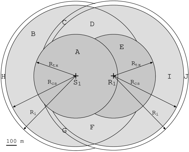
Figure 2: Communication ranges for a Lucent Orinoco 802.11b card in outdoor environment, with a sending rate of 2 Mbits/s [16].

• If the station $S_{2}$ is in the area $A$, carrier sensing and backoff allow to share the medium between $S_{1}$ and $S_{2}$.

• If the station $S_{2}$ is in the area $E$, it is commonly called hidden station [17], and the RTS/CTS mechanism will prevent the collision on $R_{1}$.

• If $S_{2}$ is in the area $I\cup J$, the sending of $S_{1}$ and $S_{2}$ will lead to some collisions on $R_{1}$ even if the RTS/CTS mechanism is used. Since $R_{1}$ will not acknowledge frames sent by $S_{1}$, $S_{2}$ will increase its contention window.

• If $S_{2}$ is in the area $B$, then it will receive the frames of $S_{1}$ without understanding them and will presume erroneous frames. As a consequence, it will wait an EIFS delay instead of a DIFS one, allowing $R_{1}$ to send the acknowledgment to $S_{1}$.

• If $S_{2}$ is in the area $D\cup F$, then it will receive the frames of both $S_{1}$ and $R_{1}$ without understanding them and wait an EIFS delay.

• If $S_{2}$ is in the area $C\cup G$, then it will receive the frames of $S_{1}$ without understanding them, and will use the EIFS delay. But it may also perturb the sending of some frames by $R_{1}$ (CTS and ACK), leading to a contention window increasing on $S_{1}$.

• Finally, if $S_{2}$ is in $H$, then its sending will create some collisions on $S_{1}$ during the reception of the CTS and ACK frames sent by $R_{1}$, and $S_{1}$ will increase its contention window.

3.2 Fairness in a chain of senders

In this paper, we study the fairness in a chain of senders, where each sender has one or several receivers which are not themselves senders (see Figure 1): a sender continuously sends some data frames to one of its neighbors, not necessarily always the same. As explained previously, several kinds of interaction can appear between neighbor senders and in some case their receivers. However many studies have already be done on the increase of the contention window. In this paper, we focus on the impact of the EIFS delay, which appears when a sender is in the area $B\cup C\cup D\cup F\cup G$ (see Figure 2) of its neighbors, combined with the chain topology.

For the purpose of our study, we suppose that each sender is in the area $B$. We noticed that very similar results are obtained when the sender is in the area $D\cup F$, but the system stabilizes much slowly. Moreover, as our simulations have been done with network simulator [18] (see Section 4), the interferences which may appear in the areas $C\cup G$ could not be taken into account.

This chain of senders scenario could rarely happen in a wireless LAN network were the mobile nodes share an access point, because in such a situation the stations are generally in the transmission range of either the sender or the receiver (i.e.. $A\cup E$ in Figure 2). But it could appear more often in ad hoc network when the nodes are widely spread in the space, and when they are moving. More fundamentally, as we will see, this case study allows some interesting conclusions on the IEEE 802.11 standard.

3.3 The three pairs fairness problem

In [1, 14], a specific scenario has been studied, where strong inequity appears. It is based on asymmetry between some pairs of communicating nodes, and on the use of the EIFS delay. In this scenario, three pairs of communicating nodes are considered. In each pair $i$ ($1\leq i\leq 3$), the sender $S_{i}$ and the receiver $R_{i}$ are close enough to establish a communication. Moreover, the sender $S_{i}$ has many data to send to the receiver $R_{i}$ in the same pair so that it always tries to gain access to the medium. The three pairs are placed in such a way that the senders can detect an emission in a neighbor pair without understanding the emission.

This is a particular case of our chains of transmitters scenario, as depicted for instance in Figure 1. Here, there is a single receiver per sender. These pairs of senders-receivers are not necessarily arranged on a line, but a sender is in the carrier sense area of its neighbors.

Simulations have been done in [1] as well as real experiments confirming the simulations. Figure 3 displays simulations results of a chain of three pairs of senders-receivers, with the parameters we will use in the following section. As already shown in [1] (with different parameters), we notice a strong inequity: the two external pairs can reach a throughput larger than 1.55 Mbits/s, whereas the central pair has a throughput which does not exceed 0.04 Mbits/s. Note that in the same conditions, the throughput of a single pair is equal to 1.59 Mbits/s.

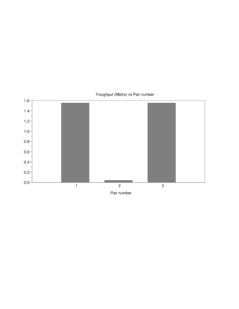
Figure 3: Fairness problem with three pairs.

To explain these results, one can remark that the central pair has to compete with two neighbors to access the channel, and then a smaller throughput than the border pairs (which have only to compete with one neighbor) is expected. Moreover, the EIFS mechanism applies as soon as a neighbor is sending, and this happens more frequently for the central pair.

4 Simulation of a chain of senders

In the previous section, we introduced the chain of senders scenario, which includes the three pairs fairness problem studied in [1, 14]. In such a scenario, the central pair has many difficulties to gain access to the channel compared to its two neighbors. But if those neighbors have more than one competitors, this could help the central pairs. In the following we study by simulation the impact of the number of pairs on the fairness in the chain of senders. This scenario combines both the EIFS mechanism and the border effect of the chain (some nodes have a single neighbor while some others have two), which is expected to be less and less important when the minimal distance to a border pair increases.

4.1 Configuration and parameters

Our simulations have been done using Network Simulator v2.28 [18], with parameters described previously and corresponding to a Lucent Orinoco 802.11b device (see Section 2 and Figure 2). Without loss of generality, we assume a single receiver per sender, leading to a chain of senders-receivers pairs. These pairs are arranged as shown in Figure 4. Similar results should be obtained with a less regular pattern (Figure 1), provided that the condition described in the chain of senders scenario introduced in Section 3 are fulfilled.

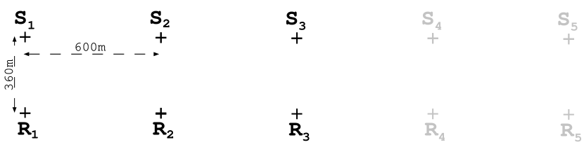
Figure 4: Chain of sender-receiver used for the simulations.

The data rate has been fixed to 2 Mbits/s, which corresponds to the Figures 2 and 4. Each sender always tries to send some UDP packets corresponding to a 1500 bytes MAC frame (see Section 2), using the RTS/CTS mechanism. Note that we did not notice a significant influence of RTS/CTS mechanism. The propagation model is the two-ray ground, corresponding to an outdoor environment with a single reflection on the ground. Others parameters are: transmission power (15 dBm), antenna height (0.9 m), receiving threshold (-91dBm), carrier sense threshold (-100dBm) [16]. The next sections show some results when the number of pairs is varying.

4.2 Fairness in a chain of four pairs

Figure 5 displays simulation results for a chain of four pairs. We observe a different behavior than with three pairs (Figure 3). The external pairs have a throughput around 1.06 Mbits/s, whereas the two central ones reach only 0.53 Mbits/s. As previously said, this difference is explained by the number of competitors: a single for the border pairs, and two for the central ones.

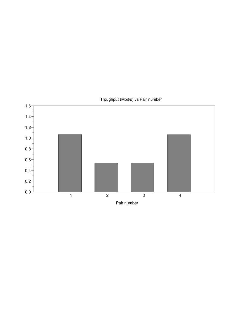
Figure 5: Fairness problem with four pairs.

Fairness is better than with three pairs because when the pair 1 acquires the channel, pair 2 is waiting and then pairs 3 and 4 have both a single competitor. By comparison with the three pairs chain, when the pair 1 acquires the channel, the other border pair always gains access to the channel. Hence, with four pairs, the central pairs can have a more frequent access to the channel than the central pair in a chain of three pairs.

Note however that when the pair 2 gains access to the channel, pairs 1 and 3 are waiting and then pair 4 acquires the channel without difficulties. This explains the difference between central pairs and border pairs.

4.3 Fairness in a chain of five pairs

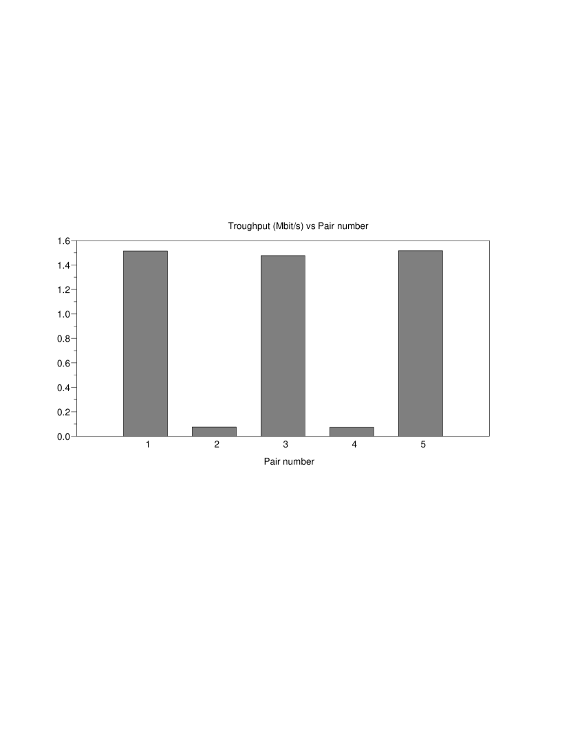
Figure 6: Fairness problem with five pairs.

Simulation results for five pairs are given in Figure 6. As we can see, pairs 1, 3 and 5 have throughputs close to the maximum, whereas pairs 1 and 2 have very low throughputs. Indeed, when the pair 1 gains access to the channel, the pair two is waiting and the pairs 3, 4 and 5 have a similar behavior than a three pair chain.

We observed a similar phenomenon with 7, 9 and 11 pairs.

4.4 Fairness in a chain of six pairs

Simulation results for six pairs are given in Figure 7. They are not so far than results for four pairs, except that pairs 2 and 5 have less bandwidth than central pairs 3 and 4, and that central pairs in the chain of four pairs. Here, even if the border pair 6 acquires the channel, pair 2 could have more than one competitor, which is not the case in a chain of four pairs. Note that the pattern can also be seen as two neighbors chains of three pairs.

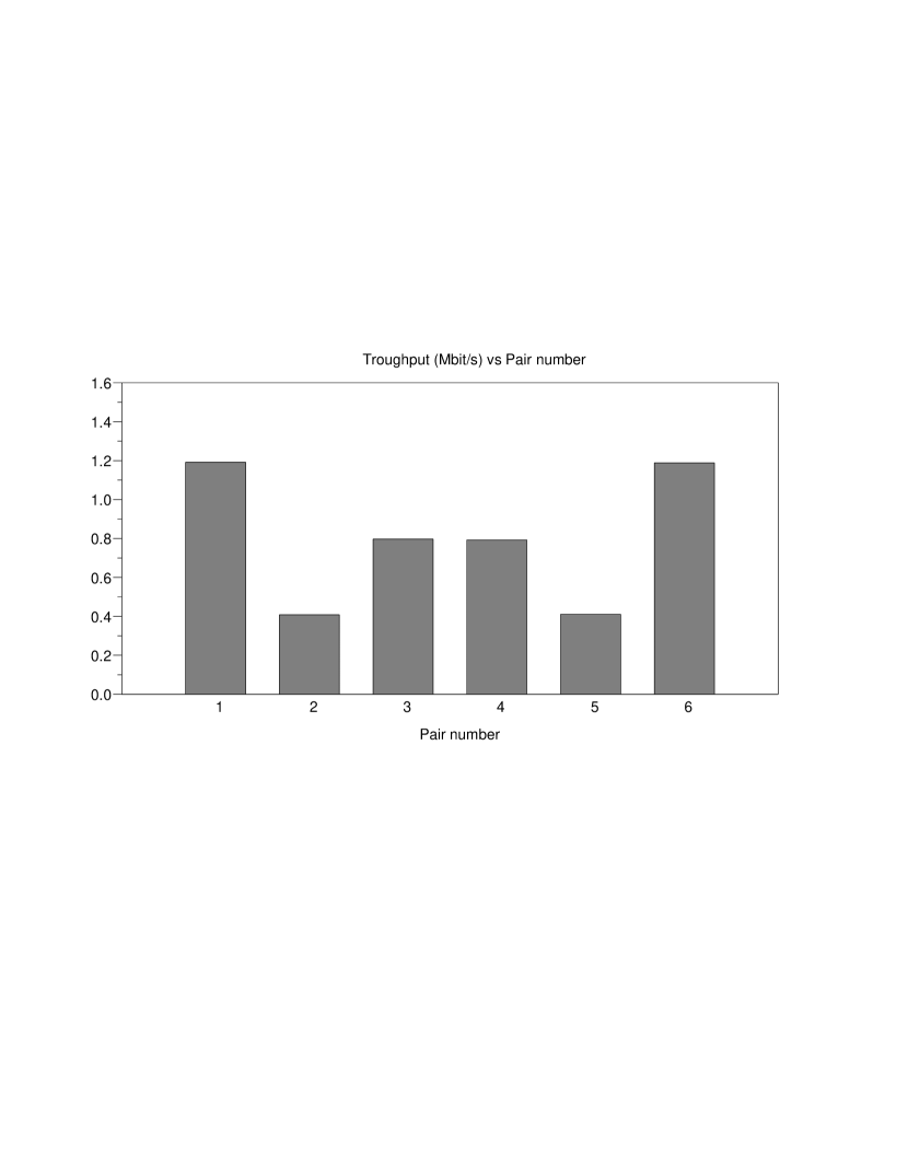
Figure 7: Fairness problem with six pairs.

We observed some similar behaviors for the chains with a larger even number of pairs, as seen in Figure 8 with eight pairs.

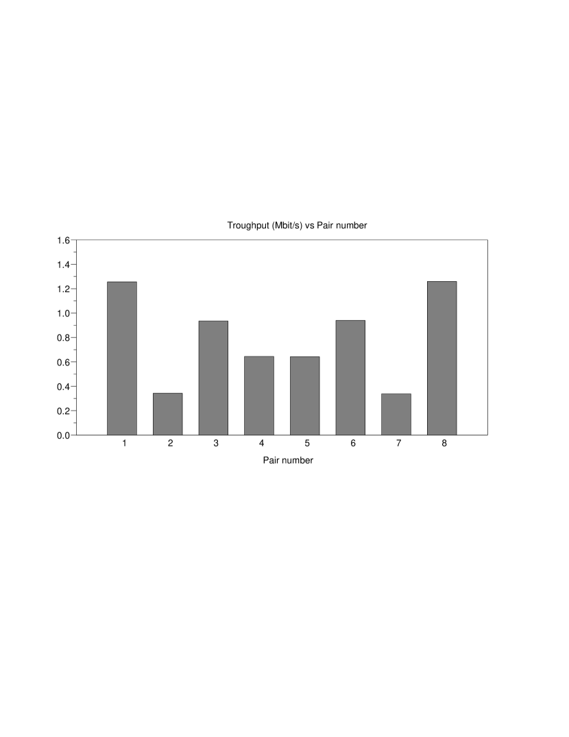
Figure 8: Fairness problem with eight pairs

4.5 Fairness in a chain of one hundred pairs

As explained below, the fairness pattern in a chain of $n$ pairs depends on the parity of $n$, which is an interesting phenomenon. When $n$ is odd, the fairness is bad (Figures 3 and 6). When $n$ is even, some more complex patterns appear with better fairness (Figures 7 and 8).

However we also observed some evolutions of these patterns when $n$ increases. We then simulated a very large chain, in order to have an idea of the asymptotic behavior.

Figure 9 displays the simulation results for a chain of one hundred of pairs. We observed that the same result is obtained with a chain of 101 pairs, which confirms that the influence of the parity of $n$ tends to decrease when $n$ increases. Moreover, for a chain of 101 pairs, one can see that the closer is an even pair from the middle, the larger is its throughput. This is explained by the fact that the influence of the border pairs is less important. As a consequence, the closer is an even pair from a border, the smaller is its throughput.

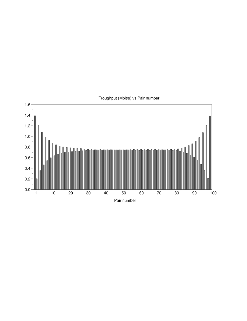
Figure 9: Fairness problem with one hundred pairs.

In this chain, the throughput of external pairs (1.39 Mbits/s) is very close to the maximum (1.59 Mbits/s), measured in a single pair in the same conditions. In the central flat area, the throughput of the pairs is close to 0.75 Mbits/s (about half of the throughput of the external pairs). As a consequence of the existence of this flat area, the insertion of a new pair has less influence on the throughput of other pairs when $n$ is large, and when the new pair is inserted near the middle of the chain.

5 Mathematical modeling

In the previous section, we have shown that a chain of senders presents some interesting phenomena, depending on the number $n$ of pairs in the chain, and on the parity of $n$. The three pairs fairness problem introduced in [1] appear as a sub-case of the chain of senders scenario presented in Section 3.

In this section, in order to study this phenomena and to improve the fairness, we propose a simple modeling of such a phenomenon, before comparing the model with the simulations.

5.1 Modeling with a non-linear system of equations

In [14], a mathematical modeling has been proposed for the three pairs configuration, by means of discrete time Markov chains. Such a modeling gives numerical results close to the simulations obtained with the ns-2 network simulator, and not so far from real experiments of [1]. Moreover, it allows to study the influence of some parameters variations on the fairness. However, it is not easily generalizable when the number of pairs increases. Indeed, a state of the Markov chain needs to capture the relative remaining backoff delays of the pairs, which leads to many states. Moreover, transitions are more complex when the number of pairs (and then interactions) increases.

We propose a new modeling, based on a non-linear systems of $n$ equations whose solution gives the probabilities of emission of each pair. It allows an analytical study both for small and large values of the number $n$ of pairs.

Let us consider a chain of $n$ pairs numbered from $1$ to $n$. For the purpose of the modeling, we admit that there are two border pairs (pair $0$ and $n+1$), which never send data.

We consider the random process $y_{i}(t)$ taking value $1$ if the $i^{\mathrm{th}}$ pair is sending data at time $t$ and 0 if the pair is idle. In fact for any $t$, the random variable $y_{i}(t)$ follows a Bernouilli’s law. We now make a simple analysis of the communication mechanism in order to obtain some relationships between the variables $y_{i}(t)$, for $i=1\dots n$.

Some data can be sent in a given pair $i$ only if its neighbor pairs are idle. Thus we have the implication

$$y_{i}(t)=1\Longrightarrow y_{i-1}(t)=y_{i+1}(t)=0.$$ (1)

But before emitting, the sender first waits after delays and CTS frames, so the converse of (1) is not true. To take this into account, we introduce a new random process $z_{i}(t)$ such that

$$P\left(z_{i}(t)=1\left|y_{i-1}(t)=y_{i+1}(t)=0\right.\right)=\alpha,$$

where $0<\alpha<1$ and we consider that data can be sent in pair $i$ at time $t$ if neighbor pairs are idle and $z_{i}(t)=1$. Thus we can write the algebraic relationship

$$y_{i}(t)=z_{i}(t)\left(1-y_{i-1}(t)\right)\left(1-y_{i+1}(t)\right),~{}i=1\dots n.$$ (2)

Since we want to describe some average behavior, we consider the rate of emission as the limit when $T\rightarrow\infty$ of the time elapsed in the emitting state between $t=0$ and $t=T$ divided by $T$

$$x_{i}=\lim_{T\rightarrow\infty}\frac{1}{T}\int_{0}^{T}y_{i}(t)\,dt.$$

In virtue of the Limit Central Theorem we have $x_{i}=E[y_{i}(t)]$, where $E[.]$ denotes the mathematical expectation, and we have of course

$$E[y_{i}(t)]=P(i\mbox{ is emitting at time }t),$$

since $y_{i}(t)$ follows a Bernouilli’s law. Hence, we can take the mathematical expectation on both sides of (2), and we obtain, by neglecting the correlation between pairs $i-1$ and $i+1$

$$x_{i}=\alpha(1-x_{i-1})(1-x_{i+1}),~{}i=1\dots n.$$ (3)

5.2 Analytical results

The modeling introduced above allows to obtain, by substitution of unknowns and by using symmetry relationships, a closed form of probabilities of emission, at least for small values of $n$. For instance, for $n=3$, we have:

$$x_{1}=\frac{2\alpha^{2}-1+\sqrt{(1-2\alpha^{2})^{2}-4\alpha^{3}(\alpha-1)}}{2\alpha^{2}}$$

For $n=4$, we have:

$$x_{1}=\frac{1+\alpha-\sqrt{(1-\alpha)(1+3\alpha)}}{2\alpha}$$

Similar expressions can be found for other pairs, but for $n>8$, there is no analytical formula because using the substitution technique leads to a polynomial with degree greater or equal than $5$, and the solution of (3) has to be computed with numerical techniques.

5.3 Validation with ns-2 results

In order to compare these results with those given by the ns-2 network simulator, we normalize both results by the value of the first external pair. Indeed, during a period of $t$ seconds, the $i^{\mathrm{th}}$ pair can send data during $t_{i}=x_{i}\times T$ seconds. Let $r_{i}$ be the sending rate of the $i^{\mathrm{th}}$ pair determined by ns-2, in bits/seconds. We have $r_{i}\times T=r_{max}\times t_{i}$ where $r_{max}$ represents the maximal sending rate depending on the configuration and $t_{i}$ the total time during which the $i^{\mathrm{th}}$ pair has sent data. Thus $r_{i}/t_{i}$ is a constant equal to $r_{max}/T$, and we have $r_{i}/t_{i}=r_{1}/t_{1}$ and then $r_{i}/r_{1}=t_{i}/t_{1}=x_{i}/x_{1}$. We then compare the throughputs of each pair divided by the throughput of the first one ($r_{i}/r_{1}$) with the probability of emission of each pair divided by the probability of emission of the first one ($x_{i}/x_{1}$).

We have done a least squares fitting with respect to $\alpha$ to approximate the ns-2 results. For instance, for $n=3$, $n=5$ and $n=7$, we obtain values of $\alpha$ respectively equal to $0.862$ and $0.838$ and $0.812$. These values of $\alpha$ lead to numerical results very close to those obtained with ns-2 network simulator, as seen in Figure 10 (a discussion of these values is given in Section 7). The slightly differences are insignificant compared to the unavoidable approximations of the network simulator. Nevertheless, this first observation is only a rough validation of our modeling, and a precise analysis of the model itself is necessary.

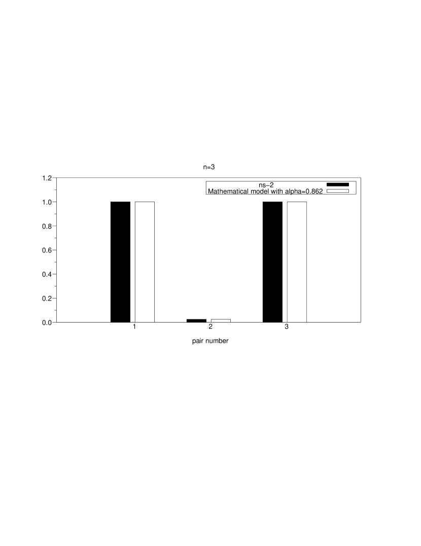
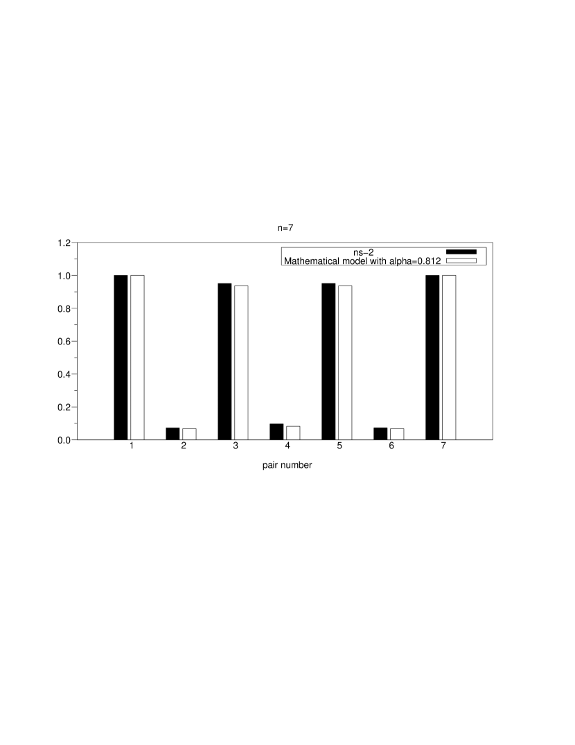
Figure 10: Comparison of $ns-2$ results and mathematical modeling for $n=3$, $5$ and $7$.

6 Analysis of the model

Our simple modeling of the chain of senders scenario fits very well with the simulations results for some given values of $\alpha$ (that we discuss in Section 7). In this section, we use this modeling to determine the asymptotic behavior of the chain, as well as to establish the relationship between $\alpha$ and the fairness.

6.1 Proving the existence of a solution

Let us consider the $n$ values $x^{k}_{1}\ldots x^{k}_{n}$ as the components of the vector $x^{(k)}\in\mathbb{R}^{n}$, and the iterative process by means of a function $F_{\alpha}$ defined on vectors:

$$x^{(k+1)}=F_{\alpha}(x^{(k)}).$$ (4)

We have:

$$F_{\alpha}(x)=\alpha\left(\begin{array}[]{c}1-x_{2}\\ (1-x_{1})(1-x_{3})\\ \vdots\\ (1-x_{n-2})(1-x_{n})\\ (1-x_{n-1})\end{array}\right).$$ (5)

The algorithm (4) is nothing but the so-called successive approximation method to determine iteratively a solution of the equation $x=F_{\alpha}(x)$. The convergence toward a unique solution $\hat{x}\in E$ is guaranteed provided the application $F_{\alpha}:E\rightarrow E$ is a contraction in some domain $E\subset\mathbb{R}^{n}$ (this is the well-known ”contraction mapping theorem”, see [19]). To show that $F_{\alpha}$ is a contraction we can use, since $F_{\alpha}$ is differentiable, the derivative $F_{\alpha}^{\prime}$ given by the matrix

$$F_{\alpha}^{\prime}(x)=\alpha\left(\begin{array}[]{ccccc}0&-1&0&0&0\\ x_{3}-1&0&x_{1}-1&0&0\\ &\ddots&\ddots&\ddots&\\ &&1-x_{n}&0&1-x_{n-2}\\ 0&0&0&-1&0\end{array}\right).$$

If we take the supremum norm, i.e. $\|x\|=\max_{1\leq i\leq n}|x_{i}|$, we can show that $\|F_{\alpha}^{\prime}(x)\|<1$, provided that $|x_{k}-1|<\frac{1}{2\alpha},\;1\leq k\leq n$, i.e. $F_{\alpha}$ is a contraction on the subspace $E$ defined by $E=\{x\in\mathbb{R}^{n},\;\|x-\mathbf{1}\|<\frac{1}{2\alpha}$, where $\mathbf{1}=(1,\dots,1)$.

A direct application of this result is that the algorithm (4) converges to the unique solution of $x=F_{\alpha}(x)$ e.g. by taking $x^{(0)}=(1,\dots,1)$.

6.2 Asymptotic behavior

As for the simulations, we observe the convergence to an asymptotic behavior. And the different behaviors between odd and even values of $n$ tend to disappear when $n$ increases. Figure 11 shows the probability of emission of pairs $k=1$ to $8$ for $n=31$ and $n=32$, for $\alpha=0.75$. For much greater values of $n$, the difference between the rates of the first $n/2$ pairs for $n$ (even) and $n+1$ pairs is negligible (typically less that $10^{-5}$ for $n=100$). Thus, without loss of generality, we will continue our study by considering only even values of $n$ in the simulations.

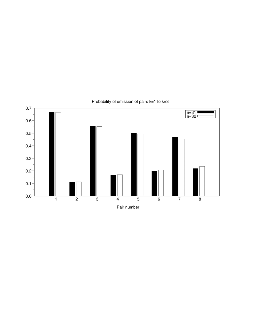
Figure 11: Simulation of probabilities of emission of pairs $k=1$ to $8$ for $n=31$ and $n=32$ ($\alpha=0.75$)

6.3 Maximization of fairness with respect to $\alpha$

Among other possible criteria (see [20] and [21]), one way of maximizing the fairness between all pairs is to maximize the entropy (see [15]) of the distribution of probability of emission $\{x_{i}\}_{i=1\dots n}$, i.e. the function

$$E(x)=-\sum_{k=1}^{n}x_{i}\log x_{i}.$$

Hence, we consider the function $J(\alpha)=\frac{1}{n}E(x(\alpha))$ where $x(\alpha)$ is the unique solution of the equation $x=F_{\alpha}(x)$ and the factor $\frac{1}{n}$ is used to allow some comparisons of results between different values of $n$.

We search for the value $\hat{\alpha}$ such that

$$J(\hat{\alpha})\geq J(\alpha),\;\forall\alpha\in[0,1].$$ (6)

The Figure 12 represents $J(\alpha)$ with respect to $\alpha$ for $n=10,20,100$ and $500$. For these values of $n$ we have respectively $\hat{\alpha}=0.5536,0.5977,0.6826,0.7309$.

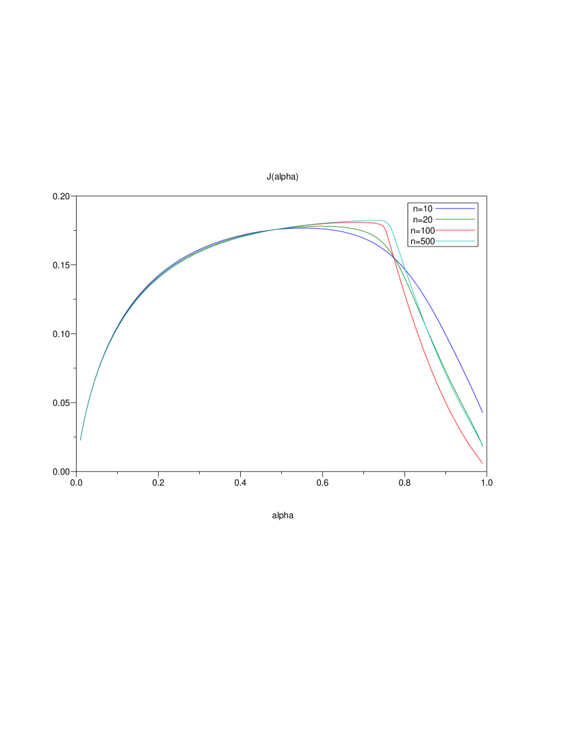
Figure 12: $J(\alpha)$ with respect to $\alpha$ for $n=10,20,100$ and $500$

The derivative of $J(\alpha)$ with respect to $\alpha$ is computed by using the classical adjoint state method, i.e. we consider the Lagrangian

$$L(\alpha,x,\lambda)=\frac{1}{n}E(x)+\lambda^{\top}(x-F_{\alpha}(x)),$$

where $\lambda$ is a vector of $\mathbb{R}^{n}$ and $\top$ denotes the transposition. The function $F_{\alpha}$ has been defined in Equation (5). We have, of course, $J(\alpha)=L(\alpha,x(\alpha),\lambda)$ for any $\lambda$. We choose $\lambda=\lambda(\alpha)$ such that

$$\frac{\partial L}{\partial x}(\alpha,x(\alpha),\lambda(\alpha))=0,$$

which leads to $\lambda(\alpha)=\frac{1}{n}[F_{\alpha}^{\prime}(\alpha)-I]^{-1}\nabla E(x(\alpha))$, where $\nabla E$ is the gradient of $E(x)$ with respect to $x$. We have finally

$$J^{\prime}(\alpha) = -\lambda(\alpha)^{\top}\left(\frac{\partial L}{\partial\alpha}F_{\alpha}(x(\alpha))\right),$$ (7)

$$= -\frac{1}{\alpha}\lambda(\alpha)^{\top}F_{\alpha}(x(\alpha)).$$ (8)

The computation of $x(\alpha)$ is done with a Newton type method, much faster than the simple fixed point method suggested by Equation (4), and the optimization is performed by the Quasi Newton BFGS method available in Scilab (see [22]).

7 Discussion

In the previous section, the chain of senders scenario has been analyzed on the basis of the modeling introduced in Section 5. Note that as far as the mathematical model is concerned, the non-linear systems of equations (3) is obtained by assuming that the emission states of pairs $i$ and $i+1$ are independent from a probabilistic point of view. While this assumption (also assumed in [23]) may be questionable, it is relevant because our modeling considers the stationary behavior of the chain.

In this section, we discuss the asymptotic values obtained in the analysis before interpreting $\alpha$ in a practical point of view.

7.1 Asymptotic flat area

If we study the asymptotic behavior of results, we see that for large values of $n$ and the optimal value $\alpha=\hat{\alpha}$, the optimal probabilities of emission (see Figure 13) exhibit a large flat area with a value very close to $\frac{1}{3}$ (the $\frac{1}{3}$ value will be discussed below). This flat area ensures that the insertion of a new pair will not disturb the rate for close neighbors.

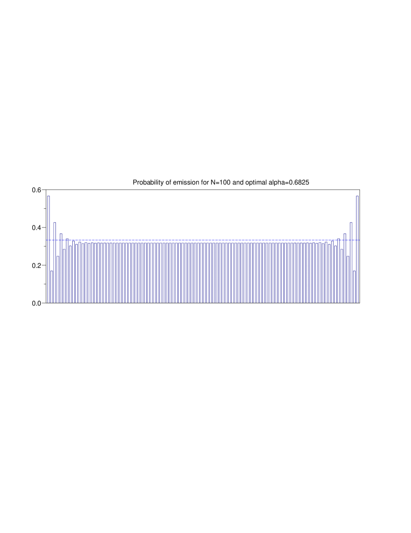
Figure 13: Probabilities of emission for $n=100$ and optimal $\alpha$. The dotted line is at probability $1/3$.

Moreover, for $n=100,500,1000$ and $2000$ the value of the optimal probability corresponding to this flat area is respectively equal to $0.3177$, $0.3290$, $0.3313$ and $0.3325$.

To understand the convergence of this value to $1/3$, we must consider the idealized situation where there is an infinite number of pairs, or equivalently, the situation where the number of pairs is large enough to allow to form a circle, where the last pair numbered $k=n$ has the pairs $k=n-1$ and $k=1$ as neighbors. Hence, there is no border effect since all pairs have two neighbor pairs.

So let us consider the $i^{\mathrm{th}}$ pair and its neighbors pairs numbered $i-1$ an $i+1$, and a very simple model of channel acquirement: each sender of each pair generates a realization of a random variable $u_{i}$ (uniformly distributed in the interval $[a,b]$). We consider that the $i^{\mathrm{th}}$ pair will acquire the channel if $u_{i}<u_{i+1}$ and $u_{i}<u_{i-1}$. The probability of this event can be calculated as follows:

$$P(u_{i}<u_{i+1},u_{i}<u_{i-1}) = \int_{a}^{b}\int_{a}^{u_{i}}\int_{a}^{u_{i}}\,\frac{d_{u_{i+1}}d_{u_{i-1}}d_{u_{i}}}{(b-a)^{3}},$$

$$= \frac{1}{(b-a)^{3}}\int_{a}^{b}(u_{i}-a)^{2}\,d_{u_{i}},$$

$$= \frac{1}{3}.$$

Hence, the value $\frac{1}{3}$ can be understood as a limiting value exhibiting the maximum fairness that can be obtained. This value of $\frac{1}{3}$ is asymptotically obtained in our model, by maximizing the entropy of the distribution of probabilities: this is a very interesting behavior.

7.2 Asymptotic optimal alpha

Another interesting phenomenon is the apparent convergence of the optimal value $\hat{\alpha}$ to $0.75$ when $n$ tends to the infinity, as it can be seen on Figure 14.

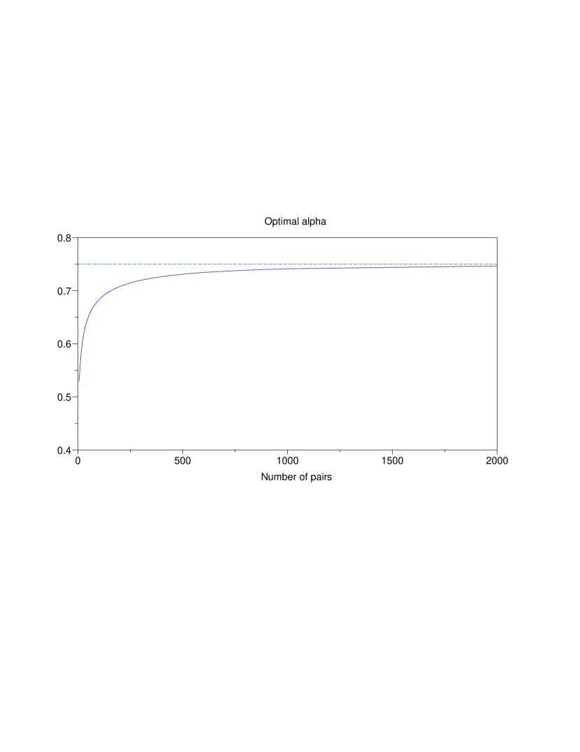
Figure 14: Optimal $\alpha$ with respect to $n$.

This is not so surprising, as we will show it in the following analysis. Consider the same idealized situation as before, where the pairs are arranged to form a circle: the probabilities of emission $\{x_{k}\}_{k=1\dots n}$ are necessarily invariant with respect to a shift of indices, since all pairs will always have two neighbors. Hence we have $x_{k}=x_{1}$, $\forall k$, and the system of $n$ equations $x=F_{\alpha}(x)$ giving the probabilities is equivalent to the scalar equation $x_{1}=\alpha(1-x_{1})^{2}$. In this case the entropy is already maximized since all values are equal. Then, if we are looking for the value of $\alpha$ giving the maximum probability of emission in such a configuration, i.e. $x_{1}=\frac{1}{3}$, we obtain $\alpha=\frac{x_{1}}{(1-x_{1})^{2}}=0.75$. This value is in fact completely determined by the topology of the neighborhood.

7.3 Asymptotic comparison of modeling and simulation

We have compared the normalized rates obtained via ns-2 and via the mathematical model for $n=100$ pairs (the rates and probabilities are normalized with respect to the pair exhibiting the maximum value, as explained in Section 5.3). On Figure 15 we can see that the mathematical model with $\alpha=0.6825$, corresponding to the maximum entropy, gives an excellent approximation of ns-2 results.

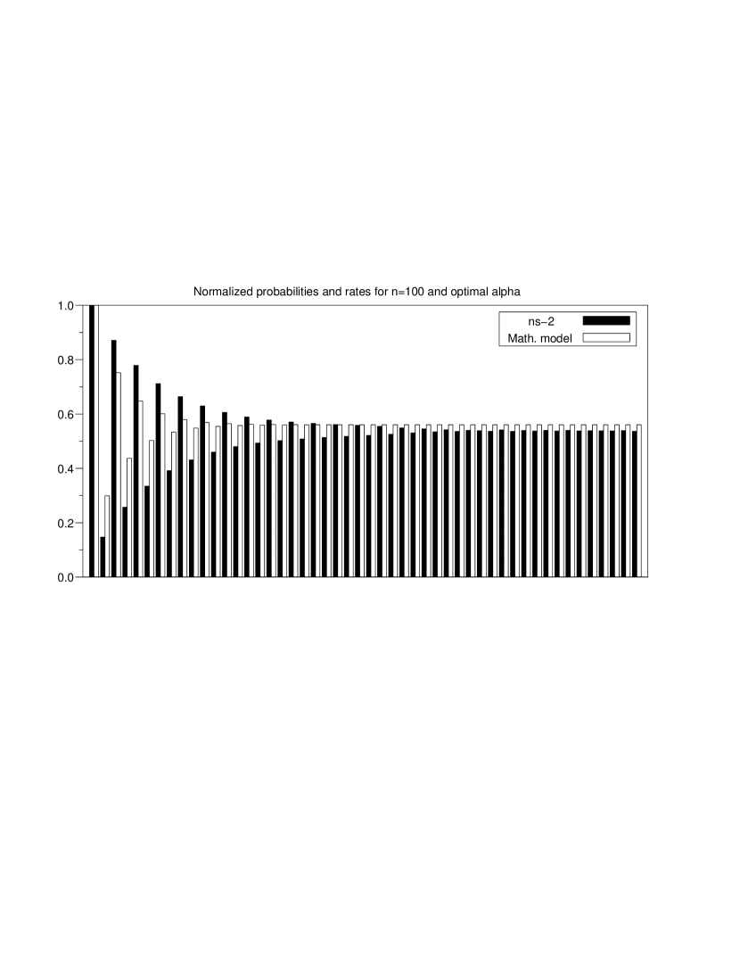
Figure 15: Probability of emission of the first $50$ pairs of 100 obtained by ns-2 and mathematical model for optimal $\alpha=0.6825$.

Hence, it appears that the asymptotic behavior of the chain of $n$ IEEE 802.11 senders-receivers (as defined in Section 4) tends to the maximum entropy when $n$ tends to the infinity. This is a surprising result.

7.4 Interpretation of the $\alpha$ coefficient

We defined $\alpha$ as the probability of sending for a given pair when its neighbors are not sending. Interpreting $\alpha$ implies to determine whether a pair is sending or not when its neighbors are not sending. This in fact depends on what is able to hear a neighbor sender, and then on what area it is on Figure 2. As for previous simulations, we suppose that the neighbors senders are in the area $B$, and that a sender can only hear transmission of a neighbor sender, and not of a neighbor receiver. A neighbor pair is then considering as sending only when the sender (and not the receiver) is sending, and waiting in other cases.

Before any transmission, a sender has to wait for a delay, and in many cases this is an EIFS delay instead of a DIFS one. During this delay, chances are large that its neighbors are sending. This means that this delay is not part of the time wasting by a pair while it could send because its neighbors are not sending. To the contrary, neighbor senders are not sending during the backoff delay.

Figure 16 summarizes a complete transmission of a $s$ bytes MAC frame between a sender $S_{i}$ and a receiver $R_{i}$ using numerical values given in Section 2 ($d$ denotes the sending rate, and 0.5 represents the mathematical expectation of a random variable on $[0,1]$).

sender $S_{i}$ receiver $R_{i}$ DIFS or EIFS 50 or 364 $\mu$s aSlotTime $\times$ CW $\times 0.5$ 310$\mu$s RTS 304 $\mu$s SIFS 10 $\mu$s CTS 352 $\mu$s SIFS 10 $\mu$s header and preamble (PHY) 192 $\mu$s $s$ data bytes (MAC) $8\times s/d$ $\mu$s SIFS 10 $\mu$s ACK 304 $\mu$s

Figure 16: Complete transmission of a $s$ bytes MAC data frame at $d$Mbits/s.

We suppose that CW = 31, leading to an average backoff time of 310 $\mu$s (we indeed rarely observed a contention window larger than 31 in our simulations, see discussions concerning the areas in Section 3). Based on the previous considerations, the waiting time $T_{w}$ while the neighbors are waiting corresponds to the backoff (310 $\mu$s), the SIFS delays ($3\times 10$ $\mu$s), the CTS (352 $\mu$s) and ACK (304 $\mu$s) frames sent by the receiver: $T_{w}=996$. The sending time $T_{s}$ while the neighbors are waiting corresponds to the RTS (304 $\mu$s) and data frame (192 + $8s/d$ $\mu$s): $T_{s}=496+8s/d$. Since $T_{s}=\alpha(T_{s}+T_{w})$, we have

$$\alpha=\frac{496+\frac{8s}{d}}{1492+\frac{8s}{d}}$$

In our simulations, the sending rate has been fixed to 2Mbits/s ($d=2$) and a data MAC frame is equal to 1500 bytes ($s=1500$). We then find $\alpha=0.867$. This value is very close to those found in Section 5.3.

7.5 Obtaining the maximal fairness

The previous equation shows a relationship between $\alpha$ and the frame size $s$. We then simulated a three pairs chain while varying the packet size. The throughput of each pair has been normalized by the reference throughput of a single pair ($1.59$ Mbits/s in our configuration) in order to compute the entropy.

Results are displayed in Figure 17. We can show that the maximum entropy is reached for a packet size of 250 bytes. This corresponds to $\alpha=0.6$, which is close to the optimal $\hat{\alpha}=0.655$.

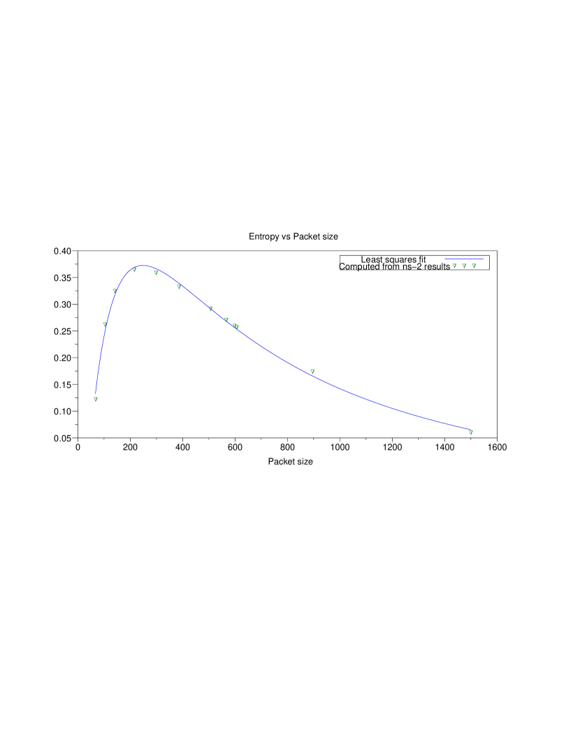
Figure 17: Entropy versus packet size.

8 Conclusion

In this paper, we developed a scenario for ad hoc networks relying on IEEE 802.11 wireless communications composed of a chain of senders, such that each of them is in the carrier sense area of its neighbors. This scenario combines the EIFS mechanism with the asymmetry of a chain, where two nodes have only one neighbor while the others have two. This scenario includes the three pairs fairness problem [1].

We show that interesting patterns appear when the number $n$ of sender-receiver pairs in the chain increases. These phenomena depend on the parity of $n$. For small values of $n$, the fairness is better if $n$ is even than if $n$ is odd. We also point out an asymptotic behavior when $n$ increases, with a large central flat area. By means of a simple modeling, we provide an analytical study of this scenario, which explains the phenomena observed by simulation. Moreover, this modeling clearly highlights a link between the fairness and the packet size.

Besides the curious fairness phenomena we pointed out in the chain of senders, it is interesting to notice that this simple modeling relying on a single coefficient $\alpha$ is able to render the complex situation of concurrent transmissions using the IEEE 802.11 standard. Previous modeling were based on Markov chains and were not really adapted for $n$ larger than 3. This coefficient expresses the probability for a sender to transmit a frame while its neighbors are waiting. Indeed, a sender does not fully use the channel, even when its neighbors are waiting.

Another interesting contribution is the asymptotic results. When the number of pairs is large, the probability of emission for a sender near the middle of the chain is very close to the optimal value (1/3). This optimal probability corresponds to $\alpha=3/4$. Moreover this value gives also the maximal fairness (expressed by means of entropy) when $n$ tends to infinity. The consequence is that, to reach the optimal case, a sender should waste 1/4 of the time it is granted for sending. We should also notice that when $n$ increases, the chain of IEEE 802.11 senders-receivers tends to this ideal case.

This ideal value of $\alpha$ is correct for very large values of $n$, which does not correspond to real cases. However, for a given $n$, the modeling is able to give the optimal $\alpha$, allowing to deduce the (approximative) optimal packet size. When applying this method on the chain of three pairs, we found an ideal MAC frame of 250 bytes. Simulation results with such a frame size lead to results very close to the optimal fairness.

Among possible further works, we would like to point out other uses of such a simple modeling, for more complex scenario.

References

- [1] D. Dhoutaut and I. Guérin-Lassous, “Impact of heavy traffic beyond communication range in multi-hops ad hoc networks,” in International Network Conference, Plymouth, July 2002.
- [2] LAN MAN Standards Comittee of the IEEE Computer Society, “Part 11: Wireless LAN medium access control (MAC) and physical layer (PHY) specifications,” The IEEE, Tech. Rep., June 1999, (reaffirmed 12 June 2003 by IEEE-SA Standard Board).
- [3] ——, “Part 11: Wireless LAN medium access control (MAC) and physical layer (phy) specifications: Higher-speed physical layer extension in the 2.4 ghz band,” The IEEE, Tech. Rep., June 1999, (reaffirmed 12 June 2003 by IEEE-SA Standard Board).
- [4] ——, “Part 11: Wireless LAN medium access control (MAC) and physical layer (phy) specifications: Higher-speed physical layer in the 5 ghz band,” The IEEE, Tech. Rep., June 1999, (reaffirmed 12 June 2003 by IEEE-SA Standard Board).
- [5] F. Cali, M. Conti, and E. Gregori, “IEEE 802.11 wireless LAN: Capacity analysis and protocol enhancement,” in IEEE Infocom, San Francisco, March 1998.
- [6] G. Bianci, “Performance analysis of the IEEE 802.11 distributed coordination function,” IEEE Journal on Selected Areas in Communications, vol. 18, no. 3, pp. 535–547, March 2000.
- [7] A. Heindl and R. German, “Performance modeling of IEEE 802.11 wireless LANs with stochastic Petri nets,” Perform. Eval., vol. 44, no. 1-4, pp. 139–164, 2001.
- [8] V. Vishnevsky and A. Lyakhov, “802.11 LANs: Saturation throughput in the presence of noise,” in IFIP-TC6 Networking Conference, Pisa, 2002.
- [9] ——, “IEEE 802.11 wireless LAN: Saturation throughput analysis with seizing effect consideration,” Cluster Computing, vol. 5, no. 2, April 2002.
- [10] V. Bharghavan, A. Demers, S. Shenker, and L. Zhang, “MACAW: a media access protocol for wireless LANs,” in ACM Sigcomm, London, August 1994.
- [11] Z. Li, S. Enandi, and A. Gupta, “Improving MAC performance in wireless ad hoc networks using enhanced carrier sensing (ECS),” in IFIP-TC6 Networking Conference, Athena, May 2004.
- [12] T. Nandagopal, T.-E. Kim, X. Gao, and V. Bharghavan, “Achieving MAC layer fairness in wireless packet networks,” in ACM Mobicom, Massachusets, August 2000.
- [13] C. Chaudet, D. Dhoutaut, and I. Guŕin Lassous, “Experiments of some performance issues with IEEE 802.11b in ad hoc networks,” in Proc. of WONS, St Moritz, January 2005.
- [14] C. Chaudet, I. Guérin-Lassous, E. Thierry, and B. Gaujal, “Study of the impact of asymmetry and carrier sense mechanism in IEEE 802.11 multi-hops networks through a basic case,” in PE-WASUN, Venice, September 2004.
- [15] E. T. Jaynes, “Information theory and statistical mechanics,” Phys. Rev., vol. 106, no. 4, pp. 620–630, 1957.
- [16] K. Xu, M. Gerla, and B. Sang, “How effective is the IEEE 802.11 RTS/CTS handshake in ad hoc networks?” in Proc. of IEEE Globecom 2002, Tapei, Taiwan, R.O.C., November 2002.
- [17] L. Kleinrock and F. Tobagi, “Packet switching in radio channels: Part I – carrier sense multiple-access characteristics,” IEEE Transactions on Communications, vol. 23, no. 12, pp. 1400–1416, 1975.
- [18] “Network simulator 2: http://www.isi.edu/nsnam/ns/.”
- [19] W. Rudin, Principles of Mathematical Analysis. New York: McGraw Hill, 1964.
- [20] C. Koksal, H. Kassab, and H. Balakrishnan, “An analysis of short-term fairness in wireless media access protocols,” in Proceeding of ACM Sigmetrics, 2000.
- [21] T. Bonald and L. Massoulié, “Impact of fairness on Internet performance,” in Proc. of Sigmetrics Performance, Cambridge, USA, 2001.
- [22] C. Bunks, J. Chancelier, F. Delebecque, C. Gomeza, M. Goursat, R. Nikoukhah, and S. Steer, Engineering and Scientific Computing with SCILAB. Birkhäuser, 1999.
- [23] C. Wang, B. Li, and L. Li, “A new collision resolution mechanism to enhance the performance of IEEE 802.11 DCF,” IEEE Transactions on Vehicular Technology, vol. 53, no. 4, pp. 1235–1246, July 2004.