Parametric instability of a magnetic junction under modulated spin-polarized current

Abstract

The stability is analyzed of the magnetic junction collinear configurations against small fluctuations under amplitude-modulated current with CPP mode. High spin injection is assumed. Under parametric resonance conditions, with the modulation frequency twice the precession frequency, instability is possible of one, or another, or both the collinear configurations. When the dc component of the current density exceeds the instability threshold of the antiparallel configuration, the parametric instability is suppressed by nonparametric one which is induced by the dc current. The parametric instability manifests itself as lowering the threshold of the dc current density in presence of the high-frequency current, such an effect has been observed in experiments repeatedly.

Studying the magnetic junctions under spin-polarized current showed a number of interesting phenomena, such as the switching of magnetic configuration [1], spin-wave generation [2], etc. Such effects may appear in nanoscale level, because the corresponding characteristic lengths, namely, the exchange length and the spin diffusion length, are of order of 10 nm [3]. This allows using the effect for high-density information recording by electric current, which is unattainable for switching magnetic elements by magnetic field alone.

The current-driven switching magnetic junctions is accompanied often with the magnetization oscillation and the other high-frequency effects (see, e.g., [2, 4, 5, 6]). In this connection, an interesting problem occurs, namely, the influence of spin-polarized high-frequency current on magnetic junctions.

The microwave effect on the switching magnetic structures by spin-polarized current was studied in Refs. [7, 8, 9, 10, 11]. Lowering threshold value of dc current density was found in presence of a high-frequency current. Nowadays, interpretation of this effect is restricted mainly with qualitative arguments and numerical simulations without developing any consistent theory. Without having pretensions to constructing a comprehensive theory, we should like to pay attention to a possible mechanism of the effect related with occurring instability of the magnetic junction configuration under parametric resonance conditions.

Let us consider a magnetic junction consisting of a pinned ferromagnetic layer 1, free ferromagnetic layer 2, and nonmagnetic layer 3 closing the electric circuit. Amplitude-modulated electric current with density

$$j(t)=\overline{j}+\widetilde{j}\cos\Omega t$$ (1)

flows perpendicular to the layers.

We assume $\widetilde{j}\leq\overline{j}$, so that the total current flows always in the same direction, corresponding to the conduction electron flux in the $1\to 2\to 3$ direction. We take, also, $\Omega\tau\ll 1$, $\tau$ being the electron spin relaxation time, that allows describing the alternative current effect by the same equations as the direct current one with changing constant current density by time-dependent one, $j(t)$.

We take a coordinate system with $x$ axis perpendicular to the layers, $yz$ plane parallel to layers, and $x$ coordinate counting off the interface between 1 and 2 layers (Fig. 1). The pinned layer magnetization vector $\mathbf{M}_{1}$ is directed along $z$ axis. The free layer magnetization vector $\mathbf{M}$ originally (without current) is collinear (parallel or antiparallel) to the pinned layer magnetization vector $\mathbf{M}_{1}=\{0,\,0,\,M_{1}\}$. We are to investigate stability of such a state in presence of the current.

Figure 1: Scheme of the magnetic junction.

The free layer thickness $L$ is assumed to be small compared to the spin diffusion length in that layer and the domain wall thickness. In such a case, the macrospin approximation is valid, in which the free layer magnetization is taken as spatially uniform, while the presence of the current is taken into account by means of additional terms proportional to the current in the equations of the motion for the lattice magnetization (see Refs. [12, 13] for detail).

In the linear approximation on small deviations of the $\mathbf{M}$ vector from the collinear position, the Landau-Lifshitz equations take the form

$$\frac{d\hat{M}_{x}}{dt}+\kappa\overline{\hat{M}}_{z}\frac{d\hat{M}_{y}}{dt}+\gamma\left(H_{z}+H_{a}\overline{\hat{M}}_{z}\right)\hat{M}_{y}$$

$$+P(t)\hat{M}_{y}+K(t)\overline{\hat{M}}_{z}\hat{M}_{x}=0,$$ (2)

$$\frac{d\hat{M}_{y}}{dt}-\kappa\overline{\hat{M}}_{z}\frac{d\hat{M}_{x}}{dt}-\gamma\left(H_{z}+H_{a}\overline{\hat{M}}_{z}+4\pi M\overline{\hat{M}}_{z}\right)\hat{M}_{x}$$

$$-P(t)\hat{M}_{x}+K(t)\overline{\hat{M}}_{z}\hat{M}_{y}=0.$$ (3)

Here $\hat{\mathbf{M}}=\mathbf{M}/|\mathbf{M}|$ is the unit vector along the free layer magnetization, $\overline{\hat{M}}_{z}=\pm 1$ is the original stationary collinear position of the vector, $\hat{M}_{x,\,y}$ are the small deviations from that position, $\mathbf{H}$ is the external magnetic field, $H_{a}$ is the anisotropy field of the free layer, $\kappa$ is the Gilbert damping constant ($\kappa\ll 1$ is assumed), $\gamma$ is the gyromagnetic ratio. We assume $|H_{z}|<H_{a}$ that excludes possibility of switching the junction by magnetic field without current.

The functions $K(t)$ and $P(t)$ describe the spin-polarized current effect for two different interaction mechanisms between the conduction electrons and magnetic lattice, namely, spin transfer torque [14, 15] and appearance of a region in the free layer with nonequilibrium electron spin polarization [16, 17]; for brevity, we name these mechanisms as torque and injection ones, respectively. Note that the contribution of the injection mechanism in the Eqs. (Parametric instability of a magnetic junction under modulated spin-polarized current) and (Parametric instability of a magnetic junction under modulated spin-polarized current) has the same form as the magnetic field, so that one may say about some effective magnetic field $H_{\rm eff}=H_{z}+P(t)/\gamma$. Note, however, that unlike the similar effect of the parametric instability under longitudinal pumping by high-frequency magnetic field [18], the spin-polarized current effect, as mentioned above, is of local nature with characteristic scale of order of the spin diffusion length $l\sim 10\div 100$ nm.

Further we consider the case of high injection when the following inequalities fulfill:

$$Z_{2}/Z_{1},\,Z_{2}/Z_{3}\ll\lambda\ll 1,$$ (4)

where

$$Z_{i}=\frac{l_{i}}{\sigma_{i}\left(1-Q_{i}^{2}\right)}\quad(i=1,\,2,\,3),$$ (5)

$l_{i}$ is the spin diffusion length for $i$th layer, $Q_{i}=(\sigma_{i\uparrow}-\sigma_{i\downarrow})/\sigma_{i}$ is the conduction spin polarization, $\sigma_{i\uparrow},\,\sigma_{i\downarrow}$ are the partial conductivities of the spin-up and spin-down electrons in $i$th layer, $\sigma_{i}=\sigma_{i\uparrow}+\sigma_{i\downarrow}$ is the total conductivity of the layer (see [19] for detail). With these assumptions, the functions $K(t)$ and $P(t)$ take the form

$$P(t)=\gamma H_{a}\frac{j(t)}{j_{0}}\equiv P_{0}+P_{1}\cos\Omega t,$$ (6)

$$K(t)=\frac{P(t)}{\alpha\tau\gamma M}\equiv K_{0}+K_{1}\cos\Omega t,$$ (7)

where $\alpha$ is the dimensionless constant of the sd exchange interaction,

$$j_{0}=\frac{eH_{a}L}{\mu_{B}\alpha\tau Q_{1}},$$ (8)

$\mu_{B}$ is the Bohr magneton, $j_{0}$ has the meaning of the threshold direct current density, which corresponds to occurring instability of the antiparallel configuration of the magnetic junction under dominating injection mechanism without external magnetic field.

Let us make the following substitution in Eqs. (Parametric instability of a magnetic junction under modulated spin-polarized current), (Parametric instability of a magnetic junction under modulated spin-polarized current):

$$\hat{M}_{x}(t)=X(t)\exp\left\{-\frac{K_{1}\overline{\hat{M}}_{z}}{\Omega}\sin\Omega t\right\},$$

$$\hat{M}_{y}(t)=Y(t)\exp\left\{-\frac{K_{1}\overline{\hat{M}}_{z}}{\Omega}\sin\Omega t\right\}.$$ (9)

The following equations are obtained for functions $X(t),\,Y(t)$:

$$\frac{dX}{dt}+\kappa\overline{\hat{M}}_{z}\frac{dY}{dt}+\left[\gamma\left(H_{z}+H_{a}\overline{\hat{M}}_{z}\right)+P_{0}\right]Y$$

$$+K_{0}\overline{\hat{M}}_{z}X=-(P_{1}-\kappa K_{1})Y\cos\Omega t,$$ (10)

$$\frac{dY}{dt}-\kappa\overline{\hat{M}}_{z}\frac{dX}{dt}-\left[\gamma\left(H_{z}+H_{a}\overline{\hat{M}}_{z}+4\pi M\overline{\hat{M}}_{z}\right)+P_{0}\right]X$$ (11)

$$+K_{0}\overline{\hat{M}}_{z}Y=+(P_{1}-\kappa K_{1})X\cos\Omega t,$$

The exponent in Eq. (Parametric instability of a magnetic junction under modulated spin-polarized current) varies within finite limits from $\exp\left\{-K_{1}\overline{\hat{M}}_{z}/\Omega\right\}$ to $\exp\left\{+K_{1}\overline{\hat{M}}_{z}/\Omega\right\}$, so that stability conditions of the zero solutions for $X(t),\,Y(t)$ coincide with those for $\hat{M}_{x},\,\hat{M}_{y}$ in the linear approximation used here.

It is seen from Eqs. (Parametric instability of a magnetic junction under modulated spin-polarized current), (11) that the torque mechanism contribution to the effects related with the alternative component of the current ($K_{1}$) appears with the small factor $\kappa$ and is absent when the damping is neglected.

Let us make the Fourier transformation in Eqs. (Parametric instability of a magnetic junction under modulated spin-polarized current), (11). The equations for the Fourier components with $\omega$ frequency take the form

$$-i\omega X(\omega)+\left[\gamma\left(H_{z}+H_{a}\overline{\hat{M}}_{z}\right)+P_{0}-i\kappa\omega\right]Y(\omega)$$

$$+K_{0}\overline{\hat{M}}_{z}X(\omega)=-\epsilon\left[Y(\omega+\Omega)+Y(\omega-\Omega)\right],$$ (12)

$$-i\omega Y(\omega)+\left[\gamma\left(H_{z}+H_{a}\overline{\hat{M}}_{z}+4\pi M\overline{\hat{M}}_{z}\right)+P_{0}-i\kappa\omega\right]X(\omega)$$

$$+K_{0}\overline{\hat{M}}_{z}Y(\omega)=+\epsilon\left[X(\omega+\Omega)+X(\omega-\Omega)\right],$$ (13)

where

$$\epsilon=\frac{1}{2}(P_{1}-\kappa K_{1}).$$ (14)

There are “shifted” Fourier components with $\omega\pm\Omega$ frequencies in the right-hand side of Eqs. (Parametric instability of a magnetic junction under modulated spin-polarized current), (Parametric instability of a magnetic junction under modulated spin-polarized current). If one writes the equations similar to (Parametric instability of a magnetic junction under modulated spin-polarized current), (11) for such components, then components with $\omega$ and $\omega\pm 2\Omega$ frequencies appear in the right-hand side of the equations. Continuing this process leads to an infinite set of equations coupled via $\epsilon$ parameter of frequency dimension. We assume this frequency to be low compared to the other characteristic frequencies of the problem, namely, the modulation frequency $\Omega$ and the system natural frequency defined below. Therefore, only the component with $\omega$ frequency may be kept in the right-hand side of the equations for the $\omega\pm\Omega$ components, so that closed set of equations is obtained.

In absence of the alternative component of the current ($\epsilon=0$), the frequency $\omega$ is determined by the zero determinant condition for the homogeneous set of equations

$$\Delta(\omega)\equiv-(1+\kappa^{2})\omega^{2}-2i\beta\omega+\omega_{0}^{2}=0,$$ (15)

where

$$\omega_{0}^{2}=\left(\Omega_{x}+P_{0}\overline{\hat{M}}_{z}\right)\left(\Omega_{y}+P_{0}\overline{\hat{M}}_{z}\right)+K_{0}^{2},$$ (16)

$$\beta=\kappa\left[\frac{\Omega_{x}+\Omega_{y}}{2}+\left(P_{0}+\frac{K_{0}}{\kappa}\right)\overline{\hat{M}}_{z}\right],$$ (17)

$$\Omega_{x}=\gamma\left(H_{z}\overline{\hat{M}}_{z}+H_{a}+4\pi M\right),\quad\Omega_{y}=\gamma\left(H_{z}\overline{\hat{M}}_{z}+H_{a}\right)$$

(usually $\Omega_{x}\gg\Omega_{y}$).

The fluctuations with frequency determined by Eq. (15) become unstable even if one of the following conditions fulfils:

$$\omega_{0}^{2}<0,\quad\beta<0.$$ (18)

In presence of the torque mechanism only ($P_{0}=0$), only the second of conditions (18) can be fulfilled at $K_{0}>\displaystyle\frac{\kappa}{2}(\Omega_{x}+\Omega_{y})$, $\overline{\hat{M}}_{z}=-1$ (the antiparallel configuration). In presence of the injection mechanism only ($K_{0}=0$), the first condition fulfils at $P_{0}>\Omega_{y}$, $\overline{\hat{M}}_{z}=-1$. By choosing the external magnetic field close enough (in magnitude) to the anisotropy field ($0<H_{a}-H_{z}\ll H_{a}$), the injection mechanism instability threshold can be lowered significantly. Such a field does not influence practically the torque mechanism threshold because of $\Omega_{x}\gg\Omega_{y}$. Under such conditions the torque mechanism may be neglecting, so that $K_{0}=0$ may be laid in Eqs. (16), (17).

We seek solution of the dispersion equation in presence of the high-frequency component in the form $\omega=\omega_{0}+\nu,\,|\nu|\ll|\omega_{0}|$. We are interesting below in stability of the solution under fulfilling the parametric resonance condition $\Omega=2\omega_{0}$.

By virtue of small $\epsilon$ parameter, we may neglect the terms in the dispersion equation where that parameter is multiplied by small quantities $\kappa$ and $\nu$.

Under actual conditions, $4\pi M\gg H_{a},\,H,\,P_{0}$ inequalities fulfill usually. With these inequalities taking into account, the following parametric resonance equation is obtained:

$$\Delta(\omega)\Delta(\omega-\Omega)=(4\pi\gamma M\epsilon)^{2}.$$ (19)

We obtain from Eq. (19)

$$\omega=\omega_{0}-2\pi i\kappa\gamma M\pm\frac{2i\pi\gamma M\epsilon}{\omega_{0}},$$ (20)

$$\omega_{0}=\sqrt{\left(\Omega_{x}+P_{0}\overline{\hat{M}}_{z}\right)\left(\Omega_{y}+P_{0}\overline{\hat{M}}_{z}\right)}$$

$$\approx\sqrt{4\pi\gamma M\left[\gamma\left(H_{z}\overline{\hat{M}}_{z}+H_{a}\right)+P_{0}\overline{\hat{M}}_{z}\right]}.$$ (21)

The following condition of the parametric instability is obtained from Eq. (20):

$$\epsilon>\kappa\omega_{0},\quad\omega_{0}^{2}>0.$$ (22)

It follows from Eqs. (18) and (22) that two instability mechanisms, namely, a nonparametric one (which is due to the spin polarized direct current in absence of modulation) and parametric one due to modulation, compete each other, so that only one of them is realized for given configuration (parallel or antiparallel). However, a situation is possible when instability of the antiparallel configuration is created by the nonparametric mechanism, while the instability of the parallel configuration is created by the parametric one. It is possible, also, that both the collinear configurations become unstable due to the parametric instability in absence of the nonparametric one. It is necessary to compare the corresponding instability thresholds to know what of the variants realizes.

The frequency $\omega_{0}$ takes different values for the parallel ($\overline{\hat{M}}_{z}=+1$) and antiparallel ($\overline{\hat{M}}_{z}=-1$) relative orientation of the pinned and free layers, these values are denoted below as $\omega_{0}^{(\pm)}$. At $|H_{z}|<H_{a}$ we have $\left(\omega_{0}^{(+)}\right)^{2}>0$. It means stability of the parallel configuration in absence of the current modulation and possibility of its instability under high enough amplitude of the high-frequency component.

From Eq. (Parametric instability of a magnetic junction under modulated spin-polarized current) with Eqs. (6), (8) and (14) taking into account, we obtain the threshold value of the alternative component amplitude $\widetilde{j}$ corresponding to occurring parametric instability

$$\widetilde{j}_{\rm th}^{(\pm)}=\frac{2e\kappa L\omega_{0}^{(\pm)}}{\mu_{B}\gamma\alpha\tau Q_{1}}.$$ (23)

At typical parameter values $\alpha\sim 10^{4}$, $\tau\sim 10^{-12}$ s, $\kappa\sim 10^{-2}$, $Q_{1}\sim 10^{-1}$, $L\sim 10^{-7}$ cm, $\omega_{0}^{(\pm)}\sim 10^{10}$ s^-1 we have $\widetilde{j}_{\rm th}^{(\pm)}\sim 10^{4}\div 10^{5}$ A/cm².

The threshold direct current density

$$\overline{j}_{\rm th}^{(\pm)}=j_{0}(1\pm H_{z}/H_{a})$$ (24)

may be both larger and smaller than $\widetilde{j}_{\rm th}^{(\pm)}$; this depends, in the first place, on the damping constant $\kappa$ and the external magnetic field. Therefore, under the mentioned condition $\widetilde{j}\leq\overline{j}$ a situation is possible when the parametric instability threshold is exceeded, while the nonparametric instability threshold still does not reached.

Note that the threshold density of the high-frequency component $\widetilde{j}_{\rm th}^{(-)}$ for the antiparallel configuration may be both smaller and larger than similar quantity $\widetilde{j}_{\rm th}^{(+)}$ for the parallel configuration; the latter situation takes place at $H_{z}<0$, $\overline{j}/j_{0}<|H_{z}|/H_{a}$.

Let us consider the case $\widetilde{j}_{\rm th}^{(-)}<\widetilde{j}_{\rm th}^{(+)}$. At $\overline{j}<\overline{j}_{\rm th}^{(-)}$, $\widetilde{j}_{\rm th}^{(-)}<\widetilde{j}<\widetilde{j}_{\rm th}^{(+)}$ the parametric instability of the antiparallel configuration takes place with stability of the parallel one; in such a case the initial antiparallel configuration switches to parallel one. At $\overline{j}<\overline{j}_{\rm th}^{(-)}$, $\widetilde{j}>\widetilde{j}_{\rm th}^{(+)}$ parametric instability of both collinear configurations occurs, so that an oscillation regime takes place. In the opposite case, $\widetilde{j}_{\rm th}^{(-)}>\widetilde{j}_{\rm th}^{(+)}$, the parametric instability of the parallel configuration takes place at $\overline{j}<\overline{j}_{\rm th}^{(-)}$, $\widetilde{j}_{\rm th}^{(+)}<\widetilde{j}<\widetilde{j}_{\rm th}^{(-)}$ and both collinear configurations at $\overline{j}<\overline{j}_{\rm th}^{(-)}$, $\widetilde{j}>\widetilde{j}_{\rm th}^{(-)}$.

At $\overline{j}>\overline{j}_{\rm th}^{(-)}$ the nonparametric instability of the antiparallel configuration occurs (because $\left(\omega_{0}^{(-)}\right)^{2}<0$); in this case, as mentioned above, parametric instability of this configuration is suppressed. However, at $\widetilde{j}>\widetilde{j}_{\rm th}^{(\pm)}$ the parametric instability of the parallel configuration takes place.

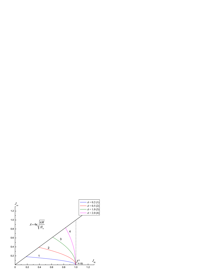
Figure 2: Phase diagram for the antiparallel configuration (see explanation in the text).

In Fig. 2 a phase diagram in $\left(\overline{j},\,\widetilde{j}\right)$ coordinates (with dimensionless variables $J_{dc}=\overline{j}/j_{0},\,J_{ac}=\widetilde{j}/j_{0}$) is shown for the antiparallel configuration at $H=0$ and various values of the parameter $A=4\kappa(\pi M/H_{a})^{1/2}$. The straight line bounds the range of the high-frequency current density values according with the condition $\widetilde{j}\leq\overline{j}$. On the right of the dashed line $J_{dc}=J_{dc\,(\rm th)}^{(-)}\equiv\overline{j}_{\rm th}^{(-)}/j_{0}$ the range is placed of the nonparametric instability of the antiparallel configuration where $\left(\omega_{0}^{(-)}\right)^{2}<0$. The parametric instability of this configuration at given value of the $A$ parameter takes place in the range between that line and the curve corresponding to that value of $A$.

Thus, instability of any of two collinear configurations, as well as both the configurations can be created under amplitude modulation of the spin-polarized current. This opens possibility of the switching any of two configurations to another (with the same direction of the total current), as well creating an oscillatory regime when both collinear configurations are unstable.

The experimentally observed lowering the threshold of switching by direct current in presence of a high-frequency component may be related with appearance of the parametric instability creating by that component under direct current density lower then the threshold mentioned.

References

- [1] J.A. Katine, F.J. Albert, R.A. Buhrman, E.B. Myers, D.C. Ralph, Phys. Rev. Lett. 84, 3149 (2000).
- [2] M. Tsoi, A.G.M. Jansen, J. Bass, W.-C. Chiang, M. Seck, V. Tsoi, P. Wyder, Phys. Rev. Lett. 80, 4281 (1999).
- [3] J. Bass, W.R. Pratt, Jr., J. Phys.: Condens. Matter 19, 183201 (2007).
- [4] I.N. Krivorotov, N.C. Emley, J.C. Sankey, S.I. Kiselev, D.C. Ralph, R.A. Buhrman, Science 307, 228 (2005).
- [5] D.C. Ralph, M.D. Stiles, J. Magn. Magn. Mater. 320, 1190 (2008).
- [6] Z.H. Xiao, X.Q. Ma, P.P. Wu, J.X. Zhang, L.Q. Chen, S.Q. Shi, J. Appl. Phys. 102, 093907 (2007).
- [7] K. Rivkin, J.B. Ketterson, Appl. Phys. Lett. 88, 192515 (2006).
- [8] Y.-T. Cui, J.C. Sankey, C. Wang, K.V. Thadani, Z.-P. Li, R.A. Buhrman, D.C. Ralph, Phys. Rev. B 77, 214440 (2008).
- [9] S.H. Florez, J.A. Katine, M. Carey, L. Folks, B.D. Terris, J. Appl. Phys. 103, 07A708 (2008).
- [10] S.H. Florez, J.A. Katine, M. Carey, L. Folks, O. Ozatay, B.D. Terris, Phys. Rev. B 78, 184403 (2008).
- [11] N. Biziere, E. Muré, J.-Ph. Ansermet, J. Magn. Magn. Mater. 322, 3320 (2010).
- [12] Yu.V. Gulyaev, P.E. Zilberman, A.I. Krikunov, A.I. Panas, E.M. Epshtein, JETP Lett. 86 328 (2007).
- [13] Yu.V. Gulyaev, P.E. Zilberman, A.I. Panas, E.M. Epshtein, J. Exp. Theor. Phys. 107, 1027 (2008).
- [14] J.C. Slonczewski, J. Magn. Magn. Mater. 159, L1 (1996).
- [15] L. Berger. Phys. Rev. B 54, 9353 (1996).
- [16] C. Heide, P.E. Zilberman, R.J. Elliott. Phys. Rev. B 63, 064424 (2001).
- [17] Yu.V. Gulyaev, P.E. Zilberman, E.M. Epshtein, R.J. Elliott, JETP Lett. 76, 155 (2002).
- [18] A.G. Gurevich, G.A. Melkov. Magnetizsation Oscillations and Waves (CRC Press, Boca Raton, FL, 1996).
- [19] E.M. Epshtein, Yu.V. Gulyaev, P.E. Zilberman, J. Magn. Magn. Mater. 312, 200 (2007).