Transformation of the angular power spectrum of the Cosmic Microwave Background (CMB) radiation into reciprocal spaces and consequences of this approach

A formalism of solid state physics has been applied to provide an additional tool for the research of cosmological problems. It is demonstrated how this new approach could be useful in the analysis of the Cosmic Microwave Background (CMB) data. After a transformation of the anisotropy spectrum of relict radiation into a special two-fold reciprocal space it was possible to propose a simple and general description of the interaction of relict photons with the matter by a “relict radiation factor”. This factor enabled us to process the transformed CMB anisotropy spectrum by a Fourier transform and thus arrive to a radial electron density distribution function (RDF) in a reciprocal space. As a consequence it was possible to estimate distances between Objects of the order $\sim$10² [m] and the density of the ordinary matter $\sim$10^-22 [kg.m^-3]. Another analysis based on a direct calculation of the CMB radiation spectrum after its transformation into a simple reciprocal space and combined with appropriate structure modelling confirmed the cluster structure. The internal structure of Objects may be formed by Clusters distant 12 [cm], whereas the internal structure of a Cluster consisted of particles distant $\sim$0.3 [nm]. This work points unequivocally to clustering processes and to a cluster-like structure of the matter and thus contributes to the understanding of the structure of density fluctuations. Simultaneously it sheds more light on the structure of the universe in the moment when the universe became transparent for photons. Clustering may be at the same time a new physical effect which has not been taken fully into consideration in the past. On the basis of our quantitative considerations it was possible to estimate the number of particles (protons, helium nuclei, electrons and other particles) in Objects and Clusters and the number of Clusters in an Object.

1 Introduction

The angular power spectrum (anisotropy spectrum) of the Cosmic Microwave Background (CMB) radiation (Sievers 2003; Hinshaw 2003) shows incredible similarity with X-ray or neutron scattering measured on non-crystalline materials (Červinka 1998, Červinka et al. 2005), see Figs. 1 and 2. Astronomers ascribe to various peaks of the anisotropy spectrum of the CMB radiation different processes (Hu 1995): It is the Sachs-Wolf effect, Doppler effect, Silk damping, Rees-Sciama effect, Sunyaev-Zeldovich effect, etc. In this connection it should be stated that all theoretical predictions of the standard cosmological model are in very good agreement with the course of the anisotropy spectrum of CMB radiation. However, the formal similarity in the form of both figures initiates the tempting idea if an analysis of the anisotropy spectrum of relict radiation using an analogous approach as is common in solid state physics, i.e. in the structural analysis of disordered materials, would bring more information on the structure of the early universe.

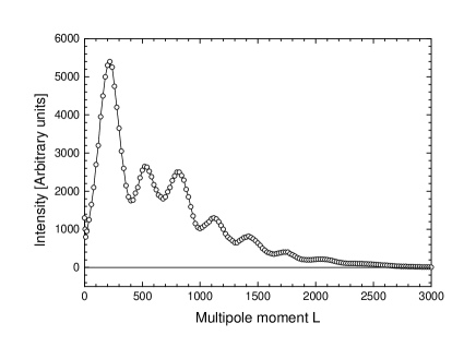
Figure 1: Anisotropy spectrum of the CMB radiation (Sievers 2003). The figure describes the dependence of the magnitude of the intensity of microwave background on the multipole moment $L=180^{\circ}/\alpha$, where $\alpha$ is the angle between two points in which the temperature fluctuations are compared to an overall medium temperature. The description of the Y-axis is for simplicity described in [Arbitrary units]. The original description was given as $L(L+1)C_{L}/2\pi$ in [$\mu$K²] units, where $L$ is the multipole moment, $C_{L}$ is a function reflecting the width of the window measuring the temperature fluctuations.

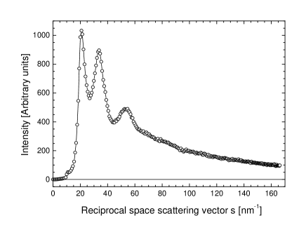
Figure 2: X-ray scattering diagram taken on a sample of a chalcogenide glass of a composition (Ge_0.19Ag_0.25Se_0.50) using the MoK_α radiation, see Červinka et al. (2005) for detail. The reciprocal space scattering vector $s$ is defined in equation (A.5).

The inspiration for this approach we found further in the nowadays situation: Although the individual disciplines in physics are highly specialized, nevertheless their methods and results are shared in areas that at the first sight may seem to be far apart. An example of this is the already established use of elementary particle physics in cosmology.

Similarly, we hope that it may be time now to apply the formalism of solid state physics to some special cosmological problems and in this way to provide an additional tool for their research. First of all our new approach may be useful in the analysis of the CMB data. We will show how after a transformation of the anisotropy spectrum of relict radiation into a special two-fold reciprocal space we will be able to process the transformed CMB anisotropy spectrum by a Fourier transform and thus calculate a radial distribution function (RDF) of Objects in a reciprocal space. Because the CMB radiation reflects the fluctuations in the density of the matter, we hope that in this way our study will be able to contribute to the understanding of the structure of these density fluctuations (Sect. 3).

Moreover this work points quite unequivocally to clustering processes and to a cluster-like structure of the matter, hence it sheds more light on the structure of the universe in the moment when the universe became transparent for photons (Sect. 4).

Clustering may be at the same time a new physical effect which has not been taken fully into consideration in the past. On the basis of our quantitative considerations it will be possible to derive the number of particles (protons, helium nuclei, electrons) in Objects and Clusters and of Clusters in an Object. This point will be demonstrated in Sect. 4.2. and discussed in Sect. 5.1.

Another analysis based on a calculation of the CMB radiation spectrum after its transformation into a simple reciprocal space, combined with appropriate modelling experiments, will confirm the cluster structure and indicate the differences between Objects and Clusters, see Sects. 4.1. and 4.2.

Moreover, we will propose on the basis of this new formalism a general description of the interaction of relict radiation with the matter. In contrast to the atomic (coherent) and Compton (incoherent) scattering factors calculated theoretically for all kinds of atoms in solid state physics, in this special case we have generated a “relict radiation factor” unifying all possible processes realized during the interaction of relict radiation with various kinds of particles, see Sects. 2.2.4. and 5.2.

2 Construction of the Classic and Relict reciprocal space

In solid state physics the principal mathematical method during the structure analysis of the matter is the Fourier transform of the intensity e.g. of X-rays or neutrons scattered by atoms building the material. The experimental data are collected in the reciprocal space and their Fourier transform brings the required information on the distribution of atoms in the real space. Now we will try to apply this approach to the CMB spectrum (see Fig. 1) and simultaneously point out the complications we have to overcome in this direction.

The necessary basic mathematical apparatus is summarized in the Appendix, the most important basic equations for the analysis of “scattered” radiation and leading to the radial density distribution function (RDF) are equations (A.1) and (A.2). The essential difference in the use of terms “scattering” and “interaction” of photons will be elucidated in the next Sect. 2.1.1.

2.1 Discussion of parameters necessary for the calculation of a radial electron density distribution

2.1.1 The relict radiation factor

During a conventional structure analysis with X-rays or neutrons, the X-ray or neutron atomic scattering factors are a precise picture of the interaction of radiation with the matter and are known precisely (Wilson & Price 1999). They enter into the calculation of the RDF in correspondence with the composition of the studied material; see equations (A.6), (A.7) and (A.10). Generally, for coherent scattering, the atomic scattering factor $f$ is the ratio of the amplitude of X-rays scattered by a given atom $E_{a}$ and that scattered according to the classical theory by one single electron $E_{e}$, i.e. $f=E_{a}/E_{e}$ ($f\leq Z$), where $Z$ is the number of electrons in the atom.

Moreover, there are scattering factors not only for the coherent but also for the incoherent (Compton) type of scattering, see e.g. later on Fig. 7.

In our study, however, the basic obstacle is that with CMB photons we have not a classic scattering process of photons on atoms; i.e. a process described in equations of the Appendix. There are not atoms, there are particles only (e.g. baryons, electrons, etc.), which participate in the formation of the structure of density fluctuations. Therefore we will speak throughout this article about an “interaction” instead of “scattering” in all cases when instead of the classic “atomic scattering factor” the new “relict radiation factor” will be used.

It is true that a part of the interaction of photons with electrons before the recombination may be realised as Thomson scattering (elastic scattering of electromagnetic radiation by a free charged particle, as described by classical electromagnetism) , but the physical background as well as the complex picture of physical processes describing the interaction of relict photons with the non uniform matter composed of various particles (electrons, ions, etc.) is not known precisely.

It is therefore evident that it will not be possible to use the conventional atomic scattering factors and that a new special factor reflecting the complexity of interaction processes of photons with the primordial matter has to be constructed. We only point out that the description of these interactions is possible only in a special two-fold reciprocal space into which the CMB spectrum is transformed. This new factor will be called the relict radiation factor and substitutes all complicated processes which participate in the formation of the angular power spectrum of CMB radiation.

In this way this approach and-or formalism may also shed some new light on the (well-known) physical processes taking place in the primordial plasma.

In order to construct the relict radiation factor we will use a basic mathematical criterion which serves well also in the classic case (see also later on Sect. 2.2.4.): Only when the atomic coherent and incoherent scattering factors (for X-rays or neutrons) are included into the calculation correctly, then the Fourier transform of the quantity $i(s)$ according equation (A.2) presents data without or with minimal parasitic fluctuations. Similarly also in this case this criterion should help us during the construction of the relict radiation factor: The relict radiation factor has to be constructed in such a way that after its insertion into the calculation of the RDF (see equations (A.1) and (A.6), where the relict radiation factor is then labelled $f_{m}$, possible parasitic fluctuations on the RDF $\rho(r)$ should be again minimized to the greatest possible extent.

The construction of the relict radiation factor is presented in Sect. 2.2.4.

2.1.2 The wavelength of radiation

The wavelength of radiation is a quantity of highest importance, too. It follows from equation (A.5), that the greater the wavelength the smaller is the maximal possible value $s_{\mathrm{max}}$ of the reciprocal space vector. At the same time the upper limit of the integral in equation (A.2) strongly influences the quality of the Fourier transform.

Although there is a broad distribution of wavelengths of photons (see later on the discussion in Sect. 5.3.) the calculation will be undertaken for the wavelength corresponding to the maximum of the wavelength distribution, i.e. for the wavelength $\lambda$ = 1.9 [mm] corresponding to the temperature 2.725 [K] of the Universe today.

That this wavelength is rational is based on three arguments. First of all photons with this wavelength bring us today the information on their last several interactions with particles, in the second place the CMB radiation spectrum is the same for all wavelengths and in the third place the wavelength corresponding to the maximum of the wavelength distribution secures the highest probability of the interaction process of photons with the matter.

2.1.3 The macroscopic density

The macroscopic density is a parameter which contributes to the calculation of the first expression on the right side of equation (A.2), i.e. it characterises “the slope” of the total disorder, see e.g. Fig.8. The calculation only of the second member of equation (A.2) may help in an estimate of this quantity, because it is highly improbable that oscillations on a properly calculated RDF should be negative. This fact has been used when estimating the density of the matter, see Sect. 3.2. It is important that the basic features of a RDF (positions of coordination spheres) are already determined by the calculation only of the second member in equation (A.2).

2.2 Preparatory calculations

2.2.1 The Classic reciprocal space

During a classic scattering experiment we measure the intensity of the scattered radiation (e.g. X-rays) as a function of the scattering angle $\theta_{\mathrm{Classic}}$. This scattering angle describes in real space the angle between the incident and scattered radiation. Its relation with the scattering vector in reciprocal space was described in equation (A.5).

On the other hand the angle $\alpha$ in the anisotropy spectrum of relict radiation (see already Fig. 1) is not a scattering angle. It is an angle characterizing a distance between an arbitrary point to another - in those different points the temperature fluctuation is measured and compared with the overall medium one.

In order to overcome the incomparableness between the angles $\theta$ and $\alpha$ we will construct an angle dependent reciprocal space to the angle $\alpha$. The basic quantity determining this reciprocal space will be the scattering angle $\theta_{\mathrm{Classic}}$.

We will suppose that the maximum possible value of the classic scattering angle $\theta^{\mathrm{max}}_{\mathrm{Classic}}=90^{\circ}$  corresponds to the maximum value of the multipole moment $L^{\mathrm{max}}$=3000.

As a consequence we receive a transformation coefficient $Q$

$$\theta^{\mathrm{max}}_{\mathrm{Classic}}=Q\,L^{\mathrm{max}}$$ (1)

(its value in this case is $Q$ = 0.03). We are then able to calculate the whole set of $\theta_{\mathrm{Classic}}$ angles

$$\theta_{\mathrm{Classic}}\,=\,L\,Q\,=\,L\>(\theta^{\mathrm{max}}_{\mathrm{Classic}}/L^{\mathrm{max}})$$ (2)

and because $L$ = 180/$\alpha$, then

$$\theta_{\mathrm{Classic}}=\frac{1}{\alpha}\,180\>(\theta^{\mathrm{max}}_{\mathrm{Classic}}/L^{\mathrm{max}})\;\;,$$ (3)

i.e.

$$\theta_{\mathrm{Classic}}=\frac{1}{\alpha}\,P_{\mathrm{Classic}}$$ (4)

where

$$P_{\mathrm{Classic}}=180\>Q\>[\mbox{deg}^{2}]$$ (5)

is a coefficient enabling the transition between space $\alpha$ and the space $\theta_{\mathrm{Classic}}$ and where the angular space $\theta_{\mathrm{Classic}}$ is reciprocal to the angular space $\alpha$ .

According equation (A.5) we are now able to construct the whole set of scattering vectors $s_{\mathrm{Classic}}$

$$s_{\mathrm{Classic}}=4\pi\,\frac{\sin\theta_{\mathrm{Classic}}}{\lambda}\;\;,$$ (6)

where $\lambda$ is the wavelength of the relict radiation. It should be noted that the quantities $s_{\mathrm{Classic}}$ and $\alpha$ are in an indirect relation. The space of the vector $s_{\mathrm{Classic}}$ will be further on called a “classic reciprocal space”.

It should be pointed out that in this construction (see equation (6)) the scattering vector $s_{\mathrm{Classic}}$ is defined in the reciprocal space (1/$\lambda$) and that this space is now dipped into the reciprocal space (1/$\alpha$), see equations (2), (4) and (6). For this “dipping” we will use further on the expression that the space $s_{\mathrm{Classic}}$ is a 2-fold reciprocal space to the space $\alpha$.

The recalculation of the original data presented in Fig. 1 using equations (4) and (6) is shown in Fig. 3. This new intensity dependence is labelled $I_{\mathrm{Classic}}(s_{\mathrm{Classic}})$.

Figure 3: Anisotropy spectrum of the relict radiation shown in Fig. 1 is recalculated as a function of $s_{\mathrm{Classic}}$, i.e. after a rescaling of the angular moment $L$ into the dependence $I_{\mathrm{Classic}}(s_{\mathrm{Classic}})$. The rescaling of the angular moment $L$ is realized on the basis of equations (2), (4) and (6) and using the MoK_α radiation wavelength $\lambda$=0.071609 [nm].

2.2.2 The Relict reciprocal space

There is a possibility to construct another reciprocal space which will be based directly on the angle $\alpha$. For a better comparison and lucidity we will use now for the angle $\alpha$ the labelling $\theta_{\mathrm{Relict}}$ i.e.

$$\alpha=\theta_{\mathrm{Relict}}\;,$$ (7)

hence

$$L=180^{\circ}/\alpha=180^{\circ}/\theta_{\mathrm{Relict}}.$$ (8)

In close analogy with equation (A.5) we now transform the anisotropy spectrum of CMB (relict) radiation into a reciprocal space (1/$\lambda$) described by the parameter $S_{\mathrm{Relict}}$

$$S_{\mathrm{Relict}}=4\pi\,\frac{\sin\theta_{\mathrm{Relict}}}{\lambda}$$ (9)

where $\lambda$ is the wavelength of the relict radiation. The space of the vector $S_{\mathrm{Relict}}$ will be further on called the “Relict reciprocal space”.

It should be noted that quantities $S_{\mathrm{Relict}}$ and $\theta_{\mathrm{Relict}}$ = $\alpha$ are in a direct relation. The anisotropy spectrum of the CMB radiation rescaled on the basis of equation (9) is here labelled $I_{\mathrm{Relict}}(S_{\mathrm{Relict}})$ and is shown in Fig. 4.

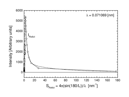
Figure 4: Anisotropy spectrum of the relict radiation shown in Fig. 1 is after a rescaling of the angular moment $L$, recalculated as a function of the Relict reciprocal space vector $S_{\mathrm{Relict}}$, into the dependence $I_{\mathrm{Relict}}(S_{\mathrm{Relict}})$. The rescaling of the angular moment $L$ is realized on the basis of equations (8), (9) and (11) using the MoK_α radiation wavelength $\lambda$ = 0.071609 [nm]. The dashed line represents a smoothed curve.

2.2.3 Relation between the Classic and Relict reciprocal space

The Classic reciprocal space was defined in equation (6), which can be rewritten, using equation (2) into an $L$-dependent form

$$s_{\mathrm{Classic}}=4\pi\,\frac{\sin(LQ)}{\lambda}$$ (10)

Similarly the Relict reciprocal space was defined in equation (9), which can be rewritten using equation (8) also into an $L$-dependent form

$$S_{\mathrm{Relict}}=4\pi\,\frac{\sin(180^{\circ}/L)}{\lambda}$$ (11)

In Fig. 5 we show the dependencies $s_{\mathrm{Classic}}(L)$ and $S_{\mathrm{Relict}}(L)$ simultaneously with the function 1/$S_{\mathrm{Relict}}(L)$.

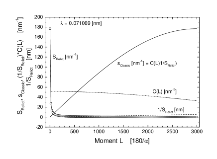
Figure 5: Mutual behaviour of reciprocal space vectors $S_{\mathrm{Relict}}$ (empty circles - equation (11)) and $s_{\mathrm{Classic}}$ (full line - equation (10)) is shown. The dependence of 1/$S_{\mathrm{Relict}}$ (dashed line) on $L$ is linear. Multiplication of 1/$S_{\mathrm{Relict}}$ by the coefficient $C(L)$, see equation (12), produces a curve lying precisely on the line $s_{\mathrm{Classic}}$. All calculations are done for the wavelength $\lambda$ = 0.071069 [nm]. See text for detail.

Now it is possible to find an $L$-dependent transformation coefficient $C(L)$ for which

$$s_{\mathrm{Classic}}\,=\,C(L)\,\frac{1}{S_{\mathrm{Relict}}}\;\;,$$ (12)

where e.g. for the wavelength $\lambda$ = 0.071069 [nm] the coefficient $C(L)$ (dimensionality [nm^-2]) has the course visualised in Fig. 5. In reality the coefficient $C$ is not only a function of $L$ but simultaneously a function of $\lambda$, i.e. precisely it should be written as $C(L,\lambda)$.

Equation (12) is important, because it enables the mutual comparison of the Classic reciprocal space (represented by vector $s_{\mathrm{Classic}}$) with the Relict reciprocal space (represented by vector $S_{\mathrm{Relict}}$) and vice versa. To summarize: the mutual relationship between the Classic reciprocal space and the Relict reciprocal space is reciprocal.

2.2.4 Construction of the relict radiation factor

Generally, a correct scattering factor has to fulfil three criterions:

(A) the $I_{\mathrm{norm}}(s)$ curve should oscillate along the $I_{\mathrm{gas}}(s)$ curve and as a consequence according equation (A.9)

(B) the curve $I_{\mathrm{distr}}(s)$ should oscillate along the zero value of the intensity axis;

(C) the resulting RDF must not be contaminated by parasitic fluctuations due to bad scaling (see Sect. A2.) as a consequence of a bad course of the scattering factor.

The mutual relation between quantities $I_{\mathrm{norm}}(s)$, $I_{\mathrm{gas}}(s)$ and $I_{\mathrm{distr}}(s)$ is explained in the Appendix, see equations (A.9), (A.10) and (B.1) with (B.2).

Figure 6: Calculation of quantities $I_{\mathrm{norm}}(s)$ - full line, $I_{\mathrm{gas}}(s)$ - dashed line (see equation (14)) and of $I_{\mathrm{distr}}(s)$ - dashed dotted line, according equations (A.9),(A.10),(B.1) and (B.2) using the “artificial” relict radiation factor $f_{\mathrm{Relict}}$ for the wavelength $\lambda$ = 0.071069 [nm]. Oscillations of the curve $I_{\mathrm{distr}}(s)$ are along the x-axis; hence all the criterions set at the beginning of this section are fulfilled. See text for details.

In Fig. 6 the calculation of the crucial curve $I_{\mathrm{gas}}$ is undertaken for the relict radiation factor $f_{\mathrm{Relict}}$. The form of this factor was determined by the trial and error method and is shown in Fig. 7. In this figure is the factor $f_{\mathrm{Relict}}$ compared with the coherent ($f^{\mathrm{X}}_{\mathrm{coh}}$) and incoherent ($f^{\mathrm{X}}_{\mathrm{incoh}}$) atomic scattering factors for X-rays corresponding to the Hydrogen atom (Wilson & Price 1999).

Similarly as for X-rays we have set the relict radiation factor $f_{\mathrm{Relict}}$

$$f_{\mathrm{Relict}}=1\quad\mbox{for}\quad s=0.$$ (13)

and further, we have set in equation (A.7) $Z$ = 1 and $m$ = 1, hence in equation (A.6) is $K_{m}$ = 1. From this point of view our construction of the relict radiation factor $f_{\mathrm{Relict}}$ should formally correspond to a “hydrogen-like” particle.

Further we have to point out that in connection with the presentation of the quantity $I_{\mathrm{gas}}(s)$ in equation (A.10) its course in Fig. 6 is given now by the relation

$$I_{\mathrm{gas}}(s)=\sum_{m}a_{m}f^{2}_{\mathrm{Relict}}\;\;.$$ (14)

In Fig. 6 we see that the function $I_{\mathrm{norm}}(s)$ is properly oscillating along the function $I_{\mathrm{gas}}(s)$ and therefore the function $I_{\mathrm{distr}}(s)$ is properly oscillating along the zero line. The consequence is that we will obtain a “proper” radial distribution function, i.e. without any parasitic maxima, see Sect. 3.1.

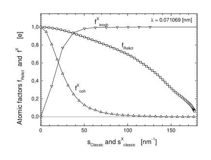
Figure 7: Behaviour of the relict radiation factor $f_{\mathrm{Relict}}$ is shown. For comparison the courses of the classic coherent and incoherent X-ray atomic scattering factors $f^{\mathrm{X}_{\mathrm{coh}}}$ and $f^{\mathrm{X}_{\mathrm{incoh}}}$ for Hydrogen are included. The parameter $s_{\mathrm{Classic}}$ is defined in equation (6), the parameter $s^{X}_{\mathrm{Classic}}$ is described in equation (A.5). Data for $f^{\mathrm{X}_{\mathrm{coh}}}$ and $f^{\mathrm{X}_{\mathrm{incoh}}}$ are taken from Wilson & Price 1999. The calculation is demonstrated for the wavelength $\lambda$ = 0.071069 [nm].

2.2.5 Relation between the Classic and Relict distribution of distances

We rewrite now the basic equation (A.2) using the scattering vector in the Classic reciprocal space $s_{\mathrm{Classic}}$, see equation (6)

$$\rho(r[\mathrm{nm}^{*}])=\rho_{\mathrm{0}}^{\mathrm{Medium}}(r)\,+\,\rho^{\mathrm{Fourier}}(r,I(s_{\mathrm{Classic}}))\;\;,$$ (15)

where $\rho_{0}^{\mathrm{Medium}}(r)$ is the member which is not Fourier-dependent and describes the structure-less total disorder depending on the density of the matter.

The parameter $r$ is measured in [nm*] in order to emphasize that the calculation of the RDF $\rho(r)$ is realized on the basis of the parameter $s_{\mathrm{Classic}}$, which is dipped in a 2-fold reciprocal space (see Sect. 2.2.1.). In other words: the calculation of the RDF $\rho(r)$ is realized in the reciprocal space of classic distances, which have the dimension [nm*]. Here we again point out the fact, that classic distances are distances between Objects calculated on the basis of the function $I_{\mathrm{Classic}}(s_{\mathrm{Classic}})$, see Fig. 3, which we analyze using equation (15).

In order to receive now the information in the real space of classic distances (characterized by the parameter $R$) we must calculate the reciprocal value of the parameter $r$ , hence the relation between $r$ and $R$ is

$$\frac{1}{r[\mathrm{nm}^{*}]}=R\,[\mathrm{nm}]\;\;.$$ (16)

It would be now possible to rewrite quite formally equation (A.2) using the scattering vector in the Relict reciprocal space $S_{\mathrm{Relict}}$, see equation (9). Similarly as for equation (15) we would receive

$$\rho(R)=\rho_{0}^{\mathrm{Medium}}(R)\,+\,\rho^{\mathrm{Fourier}}(R,I(S_{\mathrm{Relict}}))\;\;.$$ (17)

Quite hypothetically the RDF $\rho(r)$ would then bring us information on the real space of relict distances, which have the dimension [nm]. Actually, however, a RDF will not be calculated in this case, because the distribution $I(S_{\mathrm{Relict}})$, see Fig. 4, is not convenient for a Fourier transform. The calculation of relict distances in the real space, i.e. of distances between complex Objects (big clusters) will be done on the basis of a theoretical calculation of the function $I(S_{\mathrm{Relict}})$ using the Debye formula (18) calculated for appropriate models, see later on Sect. 4.

3 Calculations in the Classic reciprocal space

3.1 Calculation of RDFs

In our first example we calculate in Fig. 8 the RDF of Objects corresponding to the Fourier transform of intensities $\rho^{\mathrm{Fourier}}(r,I(s_{\mathrm{Classic}}))$ for the wavelength $\lambda$ = 0.071069 [nm], see equation (15). The scaling of intensities has been already demonstrated in Fig. 6 on the basis of the relict radiation factor $f_{\mathrm{Relict}}$ constructed in Fig. 7.

The calculated RDF shows a form typical for RDFs obtained for disordered materials. It turns out that in the region from 0.1 to 0.4 [nm*] most essential are the maxima ${}^{1}r$ and ${}^{2}r$ separated by a minimum ${}^{min}r$ , which are followed by a structure-less course. Such behaviour indicates the existence of ordering in the matter. In other words, there is a distinctive separation of the matter ending its ordering by the sphere at 0.312 [nm*] from the residual structure-less ordering starting with a plain peak at 0.395 [nm*]. The small maximum ${}^{0}r$ located at 0.172 [nm*] we consider for the present as irrelevant.

In the same way we calculated RDFs for four more wavelengths, i.e. 0.110674 [nm] ($\lambda_{\mathrm{SeK\alpha}}$), 0.154178 [nm] ($\lambda_{\mathrm{CuK\alpha}}$), 0.250466 [nm] ($\lambda_{\mathrm{VK\alpha}}$) and 0.537334 [nm] ($\lambda_{\mathrm{SK\alpha}}$). From these calculations it follows that, as expected, the dependence of the magnitude of corresponding coordination spheres on the wavelength $\lambda$ is linear, see Fig. 9, moreover, all RDFs have the same appearance.

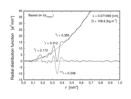
Figure 8: Calculation of the radial distribution function (RDF) according equation (15) for the wavelength $\lambda$ = 0.071069 [nm]. The dashed-dotted line corresponds to the second member in equation (15), the dashed line is the first member in this equation (dependent on density) and the full line is the sum of both components, see text for details. Value of the density $D$ necessary to shift the minimum at 0.348 [nm*] to positive values of the RDF is indicated in the upper right corner.

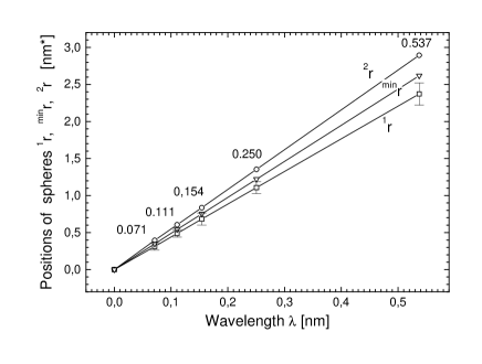
Figure 9: Dependences of most important Object distances, i.e. of coordination spheres ${}^{1}r$ (squares), ${}^{2}r$ (circles) separated by the minimum ${}^{\mathrm{min}}r$ (down triangles) on the wavelength $\lambda$ in the reciprocal space [nm*] according Fig. 8 and from analogical calculations for wavelengths 0.110674, 0.154178, 0.250466 and 0.537334 [nm]. For an easier survey error bars are inserted only for the sphere ${}^{1}r$ .

In this connection we have to point out, that the distances are measured in reciprocal space distances [nm*] and that, with respect to equation (16), these distances have to be recalculated to “real space” distances, e.g. in [km]. This recalculation is realized in Table 1, where we review the results from all wavelengths (Fig. 9) and simultaneously extrapolate the distances to the wavelength of relict radiation photons $\lambda$=1.9 [mm].

Real space distances between Objects calculated in Table 1 are visualized in Fig. 10. The extrapolation to the wavelength of relict photons 1.9 [mm] indicates that for this wavelength the shortest Object distances are in the range between 100 to 120 meters. In all further considerations, however, we will use as the most distinctive number characterizing the distance between Objects the value ${}^{2}R$ describing the start of the structure-less region, i.e. the distance ${}^{2}R$ = 98$\pm$2 [m].

Table 1: Review of most important nearest neighbour distances between Objects (${}^{1}r$ and ${}^{2}r$) separated by the minimum ${}^{\mathrm{min}}r$ on the wavelength $\lambda$ (see Fig. 8). Recalculation to real space distances $R$ is included. Simultaneously an extrapolation of distances corresponding to the wavelength of relict radiation photons 1.9 [mm] is computed together with an estimate of final errors.

Review of reciprocal space distances in [nm*] on				Recalculation of reciprocal space distances [nm*]
the basis of results presented in Figs. 7, 8 and 9				between Objects into the real space distances [km]
$\lambda$ [nm]	${}^{1}r$ [nm*]	${}^{\mathrm{min}}r$ [nm*]	${}^{2}r$ [nm*]	${}^{1}R$ [km]	${}^{\mathrm{min}}R$ [km]	${}^{2}R$ [km]
				= 1/${}^{1}r$ [nm∗-1]	= 1/${}^{\mathrm{min}}r$ [nm∗-1]	= 1/${}^{2}r$ [nm∗-1]
0.071069	0.312	0.348	0.395	3 205 128	2 873 563	2 538 071
0.110674	0.488	0.542	0.605	2 049 180	1 845 018	1 652 893
0.154178	0.682	0.752	0.836	1 466 276	1 329 787	1 136 172
0.250466	1.107	1.221	1.353	903 342	819 001	739 098
0.537334	2.372	2.618	2.895	421 585	381 971	345 423
Extrapolation to higher wavelengths $\lambda$
1	4.42	4.87	5.39	226 072	205 231	185 694
10	44	49	54	22 607	20 523	18 569
100	442	487	539	2 261	2 052	1 857
500	2 212	2 436	2 693	452	410	371
1 000	4 423	4 873	5 385	226	205	186
1 000 000	4 423 376	4 872 561	5 385 196	0.226	0.205	0.185
1 900 000	8 404 414	9 257 865	10 231 872	0.119	0.108	0.098
= 1.9	= 8.4$\pm$0.1	= 9.3$\pm$0.1	= 10.2$\pm$0.1	= 119$\pm$2	= 108$\pm$2	= 98$\pm$2
[mm]	[mm∗]	[mm∗]	[mm∗]	[m]	[m]	[m]

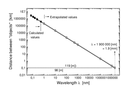
Figure 10: Dependence of real space distances between Objects, i.e. ${}^{1}R$ and ${}^{2}R$ (full squares and circles) separated by the minimum ${}^{\mathrm{min}}R$ (full up triangles) on the wavelength $\lambda$ (see Table 1 for details). Simultaneously an extrapolation to distances corresponding to the wavelength of CMB (relict) photons $\lambda$ = 1.9 [mm] is visualized (empty squares, circles and up triangles, respectively).

3.2 Calculation of the density

The calculation presented in Fig. 8 and repeated for four additional wavelengths enabled us to estimate the density of the matter, i.e. the important parameter effecting the first member $\rho^{\mathrm{Medium}}_{0}(r)$ in equation (15). We simply supposed that the fluctuations of the RDF should not be negative. In order to shift in Fig. 8 the minimum at ${}^{\mathrm{min}}r$ = 0.348 [nm*] to positive values we had to set the density to a value $D$ = 108.60 [kg.m^-3]. In the same way we have determined densities for the remaining four wavelengths.

The results are summarized in Fig. 11 and Table 2. In the log-scale is the dependence of density on the wavelength nearly linear and therefore enables again an extrapolation to higher wavelengths. This extrapolation is presented in Table 2 and visualized in Fig. 12.

It follows from Table 2 and Fig. 12 that the most probable medium density of density fluctuations of the matter with which CMB (relict) photons realized their last interaction is $D$=9$\times$10^-23 [kg.m^-3]. Taking in account the limits of our calculation then the density can be formally written as $D\sim 10^{-22}\pm 10^{-3}$ [kg.m^-3]. see also Fig. 12 and Table 2.

Figure 11: Dependence of macroscopic densities on short wavelengths. In the log-scale this dependence is nearly linear. Numerical values are given in Table 2. Numbers indicate wavelengths, for which the corresponding RDF was calculated,

Table 2: Review of numerical values of densities according Fig. 10. Extrapolation of the sequence of densities to higher wavelengths, especially to the wavelength of relict radiation photons $\lambda$=1.9 [mm] is shown. First five densities $D$ were calculated following the description in Section 3.2. Possible final error of the density $D$ is estimated and the value of the critical density $D_{\mathrm{critical}}$ according Smoot & Davidson (1977) and Silk (1977) is given.

Wavelength	Macroscopic density
$\lambda$ [nm]	$D$ [kg.m-3]
0.071069	108.6
0.110674	40.84
0.154178	17.18
0.250466	4.39
0.537334	0.46
Extrapolation to higher wavelengths $\lambda$
1	9.0 E-02
10	6.0 E-05
100	4.0 E-08
1 000	2.0 E-11
1 000 000	1.0 E-21
1 900 000
= 1.9 [mm]	9.0 E-23$\pm$E-3
Critical density:
$D_{\mathrm{critical}}$=5.0 to 7.0 E-27 [kg.m-3]

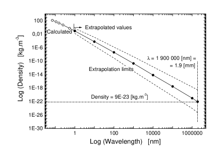
Figure 12: Extrapolation of the dependence of densities on wavelengths to the wavelength of relict (CMB) photons $\lambda$ = 1.9 [mm]. Empty circles represent values shown already in Fig. 11. Full circles are extrapolated values. Dashed lines show the limits of possible extrapolations.

4 Calculations in the Relict reciprocal space

4.1 Modelling according the Debye formula

In the case when Fig. 4 should be an X-ray scattering picture of a disordered material (e.g. of a glass) then such record would represent a picture typical for a material with well developed clusters. Their mutual distance should then characterize the position of the “first” massive peak. It follows from theory and experience that it is not possible to get from this peak information on the internal structure of Clusters, only on their magnitude and mutual distance.

The method which has to be used for an analysis of this type of scattering is a direct calculation of scattered radiation on the basis of the Debye formula

$$I(S_{\mathrm{Relict}})=\sum_{i=1}^{n}\sum_{j=1}^{n}f_{i}\,f_{j}\,\frac{\sin(d_{ij}S_{\mathrm{Relict}})}{d_{ij}S_{\mathrm{Relict}}}$$ (18)

Here $f_{i}$ and $f_{j}$ are the scattering factors of $n$ input particles and $d_{ij}$ are the distances in real space between all available particles in the model and $S_{\mathrm{Relict}}$ is the scattering vector in the Relict reciprocal space defined in equation (9). It should be pointed out that as scattering factors $f_{i}$ and $f_{j}$ we have used now the relict radiation factor $f_{\mathrm{Relict}}$ found in Sect. 2.2.4. The summation is over all $n$ particles in the model. This formula gives the average scattered intensity for an array of particles (or atoms in solid state physics) with a completely random orientation in space to the incident radiation.

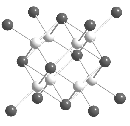
Figure 13: The basic skeleton (and-or a part of a Cluster structure) consists of 22 “positions” formed by 8 edge-bound tetrahedrons. All positions are identical, for a better graphic representation are the centres of tetrahedrons drawn white. The picture has been constructed using programs by by Petříček (2006) and Brandenburg (1999).

Our model was quite simple: For the wavelength $\lambda$ = 0.071069 [nm] the Cluster was a tetrahedron (5 particles) with an inter-particle distance 0.263 [nm] i.e. located in a cube with an edge 0.607 [nm]. In order to find the best fit with the scattering curve according equation (18), the distance between Clusters (tetrahedrons) had to be $d$ = 3 [nm], i.e. the tetrahedrons were located in positions of the basic skeleton characterized now by a side $a$ = 6.93 [nm]. This model had 22$\times$5 particles, i.e. a total of 110 particles. This calculation is shown in Fig. 14.

For all other wavelengths ($\lambda\geq$ 0.110674 [nm]) we had to increase the dimensions of the Cluster. The Cluster had then the form of the skeleton shown in Fig. 13 with an edge 0.607 [nm] and consisted of 22 particles (again with an inter-particle distance 0.263 [nm]) embedded in 8 edge-bound tetrahedrons. Only this Cluster occupied the “positions” of the cubic skeleton shown in Fig. 13 forming now an Object. (A more instructive schematic presentation of an Object is shown in Fig. 18 where Clusters are presented as small darker circles filled with “particles”.) When changing the dimension of this skeleton, we simultaneously changed again the distance $d$ between Clusters. In order to reach for $\lambda$ = 0.110674 [nm] the correct position of the massive peak at 1.6 [nm^-1] an inter-Cluster distance $d$ = 4.65 [nm] had to be used, i.e. the dimension of the skeleton was characterized by the side $a$ = 10.74 [nm]. This model had then 22$\times$22 particles, i.e. a total of 484 particles and simulated a part of the Object structure. The calculation is shown in Fig. 15.

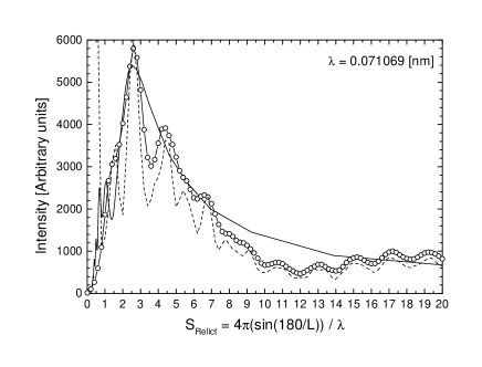
Figure 14: Calculation of the profile of the recalculated anisotropy spectrum for $\lambda$ = 0.071069 [nm] based on a set of 22 Clusters with a mutual distance $d$=3 [nm]. The Cluster was formed by a tetrahedron (5 particles); hence there were 110 particles in a model, see text for details. Full line - experiment, empty circles - calculated scaled and smoothed curve, dashed line - calculated scaled scattering.

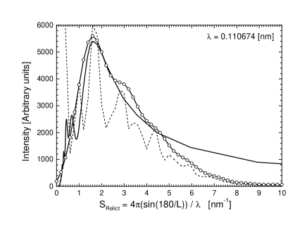
Figure 15: Calculation of the profile of the recalculated anisotropy spectrum for $\lambda$ = 0.110674 [nm] and for a set of 22 Clusters with a mutual distance of $d$=4.65 [nm]. The Cluster consisted of 22 particles, hence there were 484 particles in the model, see text for details. Full line - experiment, empty circles - calculated scaled and smoothed curve, dashed line - calculated scaled scattering.

Figure 16: Dependence of distances between Clusters on the wavelength (numerical values are shown). With exception of the “0.071 case” models consisted of 22 Clusters with 22 particles in each Cluster, i.e. a model included 484 particles. Inter-Cluster distances characterize the position of the massive peak, see Figs. 14 and 15 and the text for details.

Table 3: Extrapolation of distances between Clusters to the wavelength of relict photons 1.9 [nm]. These distances influence the position of the massive peak, see Figs. 14 and 15. The estimate of the final error is based on errors given in Fig. 16

Wavelength	Distance between Clusters
$\lambda$ [nm]	$d$ [nm]
0.071069	3.00 $\pm$ 1.50
0.110674	4.65 $\pm$ 1.00
0.154178	7.20 $\pm$ 1.00
0.250466	13.00 $\pm$ 1.00
0.537334	30.00 $\pm$ 1.00
Extrapolation to higher wavelengths $\lambda$
1	60.8
10	608
100	6 081
500	30 404
1 000	60 808
1 000 000	60 807 919
1 900 000	115 535 046
= 1.9 [mm]	$d_{\mathrm{Relict}}$=12$\pm$1 [cm]

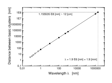
Figure 17: Extrapolation of distances between Clusters to the wavelength 1.9 [nm] - full squares; calculated values - empty squares (see Fig. 16 and Table 3).

Calculations of Cluster distances for additional wavelengths (0.154178, 0.250466 and 0.537334 [nm]) have shown (see Fig. 16) that the dependence of Cluster distances on the corresponding wavelength is linear. This fact enabled an extrapolation of the Cluster distance $d$ to the wavelength of relict photons $\lambda$=1.9 [nm], see Table 3. This extrapolated distance is $d_{\mathrm{Relict}}$= (12$\pm$1)[cm]. The extrapolation is visualized in Fig. 17.

It should be noted that the recalculated anisotropy spectrum depends in this case directly on the angle $\theta_{\mathrm{Relict}}$ which is equal to the angle $\alpha$ (see equation (8)) and therefore a recalculation of the inter-Cluster distance $d$ into a real space distance is not necessary because the Debye formula analyzes the Relict reciprocal space represented by the vector $S_{\mathrm{Relict}}$ directly in real space distances, see the quantity $d_{ij}$ in equation (18).

4.2 Quantitative relations between Objects, Clusters and particles

4.2.1 Estimates from the Object distances

We have found that the nearest distance between Objects (big clusters) is $\sim 98$ [m], see Table 1. In this moment we suppose a relatively simple organization of Objects, i.e. a “cubic body-centred” arrangement, in which an Object in the centre has 8 nearest neighbour Objects distant $b_{O}$ = 98 [m], where $b_{O}$ is the half of the body diagonal in a cube with a side

$$a_{O}=(2b_{O})/\sqrt{3}=(2\times 98\mathrm{[m]})/1.732=113.164\mathrm{[m]}.$$ (19)

The volume $V_{O}$ of this cube is therefore

$$V_{O}=1449188\mathrm{[m^{3}]}=1.449\times 10^{6}\mathrm{[m^{3}]}.$$ (20)

Using now our result on the density of the matter, see Table 2,

$$D=9\times 10^{-23}\mathrm{[kg.m^{-3}]}=m_{2O}/V_{O}$$ (21)

we are able to calculate in this model the mass $m_{2O}$ of Objects embedded in a cube with the volume $V_{O}$.

$$m_{2O} = D\times V_{O}=9\times 10^{-23}\mathrm{[kg.m^{-3}]}\times 1.449\times 10^{6}\mathrm{[m^{3}]}$$ (22)

$$= 13.04\times 10^{-17}\mathrm{[kg]}.$$

At the same time, however, we have to take in account that, as a matter of fact, there are two Objects in the space of the cube (in each cube corner there is only 1/8 of the second Object). Hence the mass $m_{O}$ embedded in one Object is

$$m_{O}=6.52\times 10^{-17}\mathrm{[kg]}.$$ (23)

A) The mass is formed by a 1:1:1 mixture of protons, helium nuclei and electrons

We may suppose now that the universe (in the time when the microwave background radiation began propagating) consisted of baryons (protons, helium nuclei, etc) and electrons, neutrinos, photons and dark matter particles. Supposing now that we have a mixture consisting of protons, helium nuclei and electrons in a relation 1:1:1, then the medium mass of a “particle” $m_{\mathrm{part}}^{1:1:1}$ in this mixture is

$$m_{\mathrm{part}}^{1:1:1} = \{(1.67\times 10^{-27}\mathrm{[kg]})+(6.64\times 10^{-27}\mathrm{[kg]})$$

$$+(0.00091\times 10^{-27}\mathrm{[kg]})\}/3,\quad\mbox{i.e.}$$

$$m_{\mathrm{part}}^{1:1:1} = (8.311/3)\times 10^{-27}\mathrm{[kg]}=2.77\times 10^{-27}\mathrm{[kg]}$$ (24)

and the number of particles $N_{\mathrm{partO}}^{1:1:1}$ in one Object is in this case

$$N_{\mathrm{partO}}^{1:1:1} = m_{O}/m_{\mathrm{part}}^{1:1:1}$$

$$= (6.52\times 10^{-17}\mathrm{[kg]})/(2.77\times 10^{-27}\mathrm{[kg]}),\quad\mbox{i.e.}$$

$$N_{\mathrm{partO}}^{1:1:1} = 2.35\times 10^{10}\quad\mbox{particles}$$ (25)

B) The mass is formed by a 1:1:10 mixture of protons, helium nuclei and electrons

Supposing now a mixture consisting of protons, helium nuclei and electrons in a relation 1:1:10, then the medium mass of a “particle” $m_{\mathrm{part}}^{1:1:10}$ in this system is

$$m_{\mathrm{part}}^{1:1:10} = \{(1.67\times 10^{-27}\mathrm{[kg]})+(6.64\times 10^{-27}\mathrm{[kg]})+$$

$$10\times(0.00091\times 10^{-27}\mathrm{[kg]})\}/12,\quad\mbox{i.e.}$$

$$m_{\mathrm{part}}^{1:1:10} = (8.319/12)\times 10^{-27}\mathrm{[kg]}=0.69\times 10^{-27}\mathrm{[kg]}$$ (26)

and the number of particles $N_{\mathrm{partO}}^{1:1:10}$ in one Object is then

$$N_{\mathrm{partO}}^{1:1:10} = m_{O}/m_{\mathrm{part}}^{1:1:10}$$

$$= (6.52\times 10^{-17}\mathrm{[kg]})/(0.69\times 10^{-27}\mathrm{[kg]}),\quad\mbox{i.e.}$$

$$N_{\mathrm{partO}}^{1:1:10} = 9.44\times 10^{10}\quad\mbox{particles}.$$ (27)

This section may be summarized by the statement that there are

$$N_{\mathrm{partO}}\approx 10^{11}\quad\mbox{particles in one Object}.$$ (28)

4.2.2 Estimates from Cluster distances

According our calculations the distance between Clusters is $\sim$12 [cm] = $1.2\times 10^{-1}$ [m], see Table 3 and Fig. 18. Similarly as in the previous case we suppose again a relatively simple organization of Clusters, i.e. a cubic body-centred arrangement in which a Cluster in the centre has 8 “nearest neighbour” Clusters distant $b_{C}=1.2\times 10^{-1}$ [m], where $b_{C}$ is the half of the body diagonal in a cube with a side

$$a_{C}=(2b_{C})/√3=(2.4\times 10^{-1}\mathrm{[m]})/1.732=1.386\times 10^{-1}\mathrm{[m]}.$$ (29)

The volume $V_{C}$ of this cube is therefore

$$V_{C}=2.66\times 10^{-3}\mathrm{[m^{3}]}.$$ (30)

Using now our result on the density of the matter, see already equation (21)

$$D=9\times 10^{-23}\mathrm{[kg.m^{-3}]}=m_{2C}/V_{C},$$

we are able to calculate for this model the mass $m_{2C}$ of Clusters embedded in a cube having the volume $V_{C}$,

$$m_{2C} = D\times V_{C}=9\times 10^{-23}\mathrm{[kg.m^{-3}]}\times 2.66\times 10^{-3}\mathrm{[m^{3}]}$$ (31)

$$= 23.94\times 10^{-26}\mathrm{[kg]}.$$

Here again we have to take in account that there are two Clusters in the space of the cube (in each corner there is only 1/8 of the second Cluster). Hence the mass $m_{C}$ embedded in one Cluster is

$$m_{C}=1.20\times 10^{-25}\mathrm{[kg]}.$$ (32)

A) The mass is formed by a 1:1:1 mixture of protons, helium nuclei and electrons

Similarly as in the preceding Sect. 4.2.1. we suppose again a mixture of protons, helium nuclei and electrons in a relation 1:1:1, respectively. The medium mass of a “particle” $m_{\mathrm{part}}^{1:1:1}$ in this mixture is (see equation (24))

$$m_{\mathrm{part}}^{1:1:1}=2.77\times 10^{-27}\mathrm{[kg]}$$

and the number of particles $N_{\mathrm{partC}}^{1:1:1}$ in one Cluster is then

$$N_{\mathrm{partC}}^{1:1:1} = m_{C}/m_{\mathrm{part}}^{1:1:1}$$

$$= (1.20\times 10^{-25}\mathrm{[kg]})/(2.77\times 10^{-27}\mathrm{[kg]}),\quad\mbox{i.e.}$$

$$N_{\mathrm{partC}}^{1:1:1} = 0.43\times 10^{2}\quad\mbox{particles}.$$ (33)

B) The mass is formed by a 1:1:10 mixture of protons, helium nuclei and electrons

Identically as in the preceding Sect. 4.2.1. the medium mass of a “particle” is in this case, see equation (26),

$$m_{\mathrm{part}}^{1:1:10}=0.69\times 10^{-27}\mathrm{[kg]}$$

and the number of particles $N_{\mathrm{partC}}^{1:1:10}$ in one Cluster is then

$$N_{\mathrm{partC}}^{1:1:10} = m_{C}/m_{\mathrm{part}}^{1:1:10}$$

$$= (1.20\times 10^{-25}\mathrm{[kg]})/(0.69\times 10^{-27}\mathrm{[kg]}),\quad\mbox{i.e.}$$

$$N_{\mathrm{partC}}^{1:1:10} = 1.74\times 10^{2}\quad\mbox{particles}.$$ (34)

This section can be summarized by the statement that there are

$$N_{\mathrm{partC}}\approx 10^{2}\quad\mbox{particles in one Cluster}.$$ (35)

4.2.3 Consequences of previous calculations

We are now able to calculate easily the number of Clusters in one Object. Because an Object consists of $N_{\mathrm{partO}}\approx 10^{11}$ particles in one Object (equation (28)) and there are $N_{partC}\approx 10^{2}$ particles in one Cluster, it follows that an Object should be composed from $N_{C}$ Clusters, where

$$N_{C}=(N_{\mathrm{partO}}/N_{partC})\approx 10^{11}/10^{2}\approx 10^{9}\quad\mbox{Clusters}.$$ (36)

Supposing that densities in the Object and in the Cluster are equal then this value is independent on the value of the density and on the mass of the particle (e.g. $m_{\mathrm{part}}^{1:1:1}$) and depends only on the relation of the volumes $V_{O}/V_{C}$, because

$$N_{C} = (N_{\mathrm{partO}}/N_{partC})=V_{O}/V_{C}$$ (37)

$$= 1.449\times 10^{6}\mathrm{[m^{3}]}/2.66\times 10^{-3}\mathrm{[m^{3}]}$$

$$\approx 10^{9}\quad\mbox{Clusters}.$$

5 Discussion

In the following discussion we will concentrate on several important ideas which may arise when reading this paper.

First of all this contribution should demonstrate how the formalism imported from solid state physics could be useful in solving specific cosmological problems: It may shed some new light on the physical processes taking place in the primordial plasma.

For example, this work points quite unequivocally to clustering processes and to a cluster-like structure of the matter in the moment when the universe became transparent for photons (see Sect. 5.1.).

Further, the new formalism enabled us a simple and general description of the interaction of relict radiation with the matter and may help in an improvement of the theoretical predictions of the CMB pattern (see Sect. 5.2.).

Finally this new approach may be useful in the analysis of the CMB data. We have shown that the transformation of the anisotropy spectrum of relict radiation into a special two-fold reciprocal space and into a simple reciprocal space was able to bring quantitative data in real space. Problems with the transformation into reciprocal spaces, mainly with the use of the proper wavelength of relict photons will be discussed in Sect. 5.3.

5.1 The cluster-like structure of the primordial matter

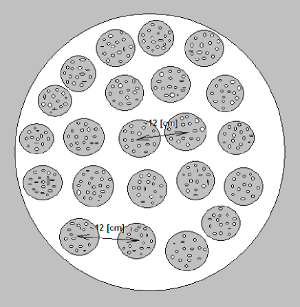
Figure 18: A schematic arrangement of Clusters (darker regions) with particles (small white points) in an Object (white region). Distance between Objects is $\sim$98 [m], see Table 1. Detailed structure of a Cluster and of an Object in our model is presented in Fig. 13. The most probable model distance between Clusters is 12 [cm], see Table 3. Distance between particles is 0.26 [nm]. There are $\sim$10¹¹ particles in one Object, $\sim$10² particles in one Cluster (see Sect. 4.2.) and $\sim$10⁹ Clusters in one Object, see Sect. 4.2.

We have already mentioned that the process of forming the primordial matter by particle clustering may be a new physical effect which has not been fully taken into consideration in the past. Now we present a model of the cluster-like structure

Concerning our results on the distances between Objects and Clusters, we have arrived to three numbers, which we interpret in a following way: The first one, which is 98 [m], (Table 1) indicates the distance between Objects (big clusters), the second one, which is 12 [cm], (Table 3) indicates the distance between smaller Clusters, while the internal structure of a single Cluster is formed by 22 particles and is characterized by a medium particle distance 0.26 [nm], see Sect. 4.1.

In Fig.18 we show a schematic picture of the cluster model. The big circle represents an Object. An Object is a clump of Clusters, where only a part of this clump was simulated in our model by 22 Clusters each having 22 particles, i.e. by a total of 484 particles in an Object.

Although this model gave a sufficiently well agreement with the width of the massive peak, as demonstrated in Fig. 15, our estimates (Sect. 4.2.) show that the number of Clusters as well as the number of particles in one Cluster is greater., i.e. that there may be as far as 10¹¹ particles in one Object and 10² particles in one Cluster. That the density plays an important role in these calculations will be discussed in Sect. 5.4.

It is important to note that the distance between Objects (${}^{2}R$=98[m], see Table 1) is not identical with the dimension of the Object as defined in Sect. 4.1. There the dimension of an Object was determined by the inter-Cluster distance $d_{\mathrm{Cluster}}$ = 0.12 [m] (see Table 3). This distance is a quarter of the body diagonal in the cube-like skeleton (with an edge $a_{\mathrm{Object}}$ = 0.28 [m]) simulating the Object according Fig. 13. The dimension of an Object is then determined by the diameter of a sphere surrounding Clusters located in the skeleton “positions”. The value of this diameter is 2$R_{\mathrm{Object}}$ = 0.48 [m], i.e. much smaller than ${}^{2}R$=98[m].

We have already mentioned (see Sect. 4.1.) that in principle it is not possible to solve on the basis of the massive peak (located e.g. at $S_{\mathrm{Relict}}$ = 1.62 [nm^-1] for $\lambda$ = 0.1107 [nm], see Fig. 15) the internal structure of a Cluster. It is possible to reach only information on the Cluster magnitude and on the distance between Clusters.

Just this information we have derived from our model calculations: The magnitude of a Cluster was based on the particle distance 0.263 [nm] and was defined by a cube with an edge $a_{\mathrm{Cluster}}$ = 0.607 [nm] (see Fig. 13), which may be surrounded by a sphere with a radius $R_{\mathrm{Cluster}}$ = 0.53 [nm], hence a diameter of a Cluster has the value 2$R_{\mathrm{Cluster}}$ = 1.05 [nm]. It is important to note that this diameter, similarly as for Objects, is not identical with the distance between Clusters (12 [cm]), see Fig. 18. However, it is this distance, which influences the position of the peak, while its intensity depends on the number of particles in the Cluster and their “mass” represented by their “scattering” power (i.e. by their relict radiation factor).

Interesting may be the effect of changing the inter-Cluster distance: A decrease of the inter-Cluster distance from 12 cm to e.g. 10 cm would bring for the 1:1:1 mixture of particles (see Sect. 4.2.2.) a value of 25 particles in one Cluster and for the 1:1:10 mixture of particles a value of 100 particles in a Cluster, i.e. numbers which roughly correspond to our model numbers in Sect. 4.1. Similarly a greater proportion of heavier particles should decrease the number of particles, thus again corresponding to the model number.

Even when the cluster model gave a good profile of the massive peak at e.g. 1.62 [nm], than such a model cannot be a unique one, because the calculation of the profile is not sensitive to the internal cluster structure, however, the cluster-like character of the modelling process has to be maintained.

How it was possible to estimate on the basis of inter-Cluster and inter-Object distances the number of particles (protons, helium nuclei, electrons) in Objects and Clusters and of Clusters in an Object was demonstrated in Sects. 4.2. and 4.3., however how these numbers are influenced by the density will be discussed in Sect. 5.4.

5.2 The relict radiation factor

We have already pointed out in Sect. 2.1.1. why during the analysis of the CMB spectrum it has not been possible to apply conventional atomic scattering factors used in solid state physics and why a new special factor reflecting the complexity of interaction processes of photons with the primordial matter has to be constructed. It is important to have in mind that the description of these interactions is possible only in a special two-fold reciprocal space into which the CMB spectrum was transformed. We have called this new factor the relict radiation factor and it had to substitute all complicated processes which participate in the formation of the angular power spectrum of CMB radiation, see Sect. 2.2.

Because relict photons realize their interaction with various kinds of particles and we have generated only one radiation factor, this factor represents, as a matter of fact, a medium from all possible individual relict radiation factors. In this way this new formalism offers a general description of the interaction of relict radiation with the matter and simultaneously reflects the complexity of processes which influence the anisotropy spectrum of CMB radiation from the cosmological point of view (Hu et al. 1995).

During our study we have concentrated on three important facts which may justify the attempt to interpret the anisotropy spectrum of CMB radiation as a consequence of the interaction of photons with density fluctuations characterizing the distribution of particles before the recombination process.

The first fact is that temperature fluctuations in the CMB spectrum are related to fluctuations in the density of matter in the early universe and thus carry information about the initial conditions for the formation of cosmic structures such as galaxies, clusters or voids (Wright 1994).

Secondly, it is the fact that the information on these density fluctuations in the distribution of particles (electrons, ions, etc.) has been brought by photons. Photons which we observe from the microwave background have traveled freely since the matter was highly ionized and they realized their last Thomson scattering (see already Sect. 2.1.1.). If there has been no significant early heat input from galaxy formation then this happened when the Universe became cool enough for the protons to capture electrons, i.e. when the recombination process started (White 1994).

The third fact is that the anisotropy spectrum is angular dependent, see Fig. 1.

Although we know that the anisotropy spectrum of CMB radiation, as presented in Fig. 1, has no direct connection with a scattering process of photons, it was the transformation of the CMB spectrum into a two-fold reciprocal space, which enabled us to interpret the anisotropy spectrum of CMB radiation as a result of an interaction process of photons with density fluctuations of the matter represented by electrons, ions or other particles. This approach enabled us to reach an advantageous approximation of this process.

The process consisted of two steps: First of all we have constructed in Sect. 2.2.1. an angular reciprocal space characterized by the “scattering” angle $\theta_{\mathrm{Classic}}$, see equations (2) and (4). This space is reciprocal to the space characterized by the angle $\alpha$ ($\alpha$ is the angle between two points in which temperature fluctuations of CMB radiation are compared to an overall medium temperature).

Then, we have constructed an additional “classic” reciprocal space (1/$\lambda$) into which the first one (the $\theta_{\mathrm{Classic}}$, space) was dipped, by defining in this new “two-fold” reciprocal space the classic scattering vector $s_{\mathrm{Classic}}$, see equation (6). Only after these transformations we treated in this new Classic reciprocal space the transformed anisotropy CMB spectrum as a scattering picture of relict photons.

It was only this space in which we simulated (in Sect. 2.2.4.) the interaction of CMB (relict) photons with density fluctuations by the relict radiation factor $f_{\mathrm{Relict}}$.

The criterion for the trial and error construction of the relict radiation factor $f_{\mathrm{Relict}}$ has been that this factor had to fulfill the three requirements set at the beginning of Sect. 2.2.4. Only then it was secured that after the Fourier transform, according equations (A.2) and-or (15), there will not be any (or at least small) parasitic fluctuations on the curve $\rho(r)$ and-or $\rho^{\mathrm{Fourier}}(r)$. That we have achieved these demands is documented in Fig. 8 where we do not see any parasitic fluctuations on the curve $\rho^{\mathrm{Fourier}}(r)$ and as a consequence on the curve $\rho(r)$.

To summarize: It is true that in our formal analogy between scattering of e.g. short-wave radiation on disordered matter (Fig. 2) and “scattering” of CMB photons on electrons, ions and other particles (Fig. 1) is an essential difference, because the physical processes are completely different, e.g. the scattering process itself, length scales involved, etc., however, the difference between physical processes is reflected and simultaneously eliminated by the special relict radiation factor $f_{\mathrm{Relict}}$ (Sect. 2.2.4.), which we have included into all calculations based on the classic two-fold reciprocal space (see Sect. 2.1.). Moreover, additional calculations in the Relict reciprocal space (see Sect. 4.) based on the relict radiation factor were done directly for the transformed angular power spectrum of relict radiation (see $I_{\mathrm{Relict}}(S_{\mathrm{Relict}})$ in Fig. 4) and thus present an information on distance relations between Clusters (formed by particles) in real space.

5.3 The wavelength problem

The problem is to which wavelength of relict photons we have to relate our calculations. One possibility may be to refer this wavelength to that time when 379.000 years after the Big Bang the Universe cooled down to 3000 K and the ionization of atoms decreased already only to 1%. Then according Wien’s law

$$\lambda_{\mathrm{max}}=\frac{b}{T}$$ (38)

where $\lambda_{\mathrm{max}}$ is the peak wavelength, $T$ is the absolute temperature of the blackbody, and $b$ is a constant of proportionality called Wien’s displacement constant, $b$ = 2.8978$\times$10^-3 [mK], we obtain for the temperature 3000 K a wavelength value $\lambda_{\mathrm{max}}$ = 966 [nm] (Šmída 2010).

However, simultaneously we must be aware of the fact that we are analyzing CMB photons now when the temperature of the universe, due to its expansion, is 2.725 K. Then the wavelength of photons according the Wien’s law should be $\sim$1 [mm].

On the other hand the COsmic Background Explorer (COBE) measured with the Far Infrared Absolute Spectrophotometer (FIRAS) the frequency spectrum of the CMB, which is very close to a blackbody with a temperature 2.725 K (Mather et al. 1994; Wright et al. 1994). The results are shown in Fig. 19 in units of intensity (see the text to Fig. 19). It follows that the wavelength corresponding to the maximum is 1.9 [mm].

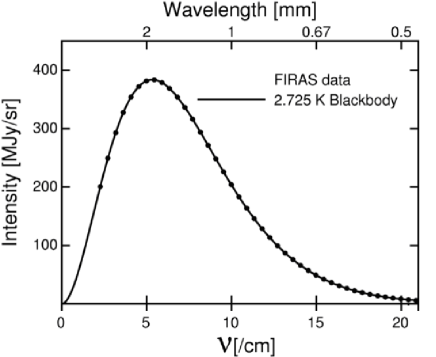
Figure 19: Dependence of the intensity of the CMB radiation on frequency as measured by the COBE Far InfraRed Absolute Spectrophotometer (FIRAS) (Mather et al. 1994; Wright et al. 1994). The thick curve is the experimental result; the points are theoretically calculated for an absolute black body with a temperature of 2.725 [K]. The x axis variable is the frequency $\nu$ in [cm^-1]. The y-axis variable is the power per unit area per unit frequency per unit solid angle in MegaJanskies per steradian (1 [Jansky] is a unit of measurement of flux density used in radioastronomy, abbreviated “Jy” (1 [Jansky] is 10^-26 [W.m^-2.Hz^-1]).

After all we have decided to relate our results to the wavelength of CMB photons 1.9 [mm] which corresponds to the maximum of the intensity distribution. Because the distribution of the spectrum covers a relatively broad interval of wavelengths, see Fig. 19, calculations based on the wavelength 1.9 [mm] should then represent the most probable calculation and estimate presented in this study. Moreover, this consideration is supported by the fact that the angular distribution of CMB radiation is the same for all wavelengths.

However, on the basis of graphs in Figs. 10, 12 and 16 an easy recalculation of distances and-or of the density would be possible when another CMB photons wavelength would be considered as more appropriate.

5.4 The density of the mass and distances between Objects, Clusters and particles

The way how we arrived to numbers characterizing the density of the matter was described in Sect. 3.2. In a conventional X-ray analysis the density is the macroscopic density of the material under study. Therefore we suppose that also in this case the density which influences the parabolic shape of the curve of total disorder (see the first member on the right side of equation (A.2) and-or (15) and Fig.8) should be understood as a real medium density of density fluctuations.

The dependence of the density on the wavelength as demonstrated in Figs. 11 and 12 is not perfectly linear; therefore we have marked in Fig. 12 the extent of possible linear dependences. This result can be formally written as

$$D=10^{-22}\pm 10^{-3}\mathrm{[kg.m^{-3}]}.$$ (39)

It follows that this medium value is about 10⁵ times higher than the “critical density” $D_{\mathrm{critical}}$ = (5 to 7)$\times$10^-27 [kg.m^-3] (Smoot & Davidson (1977), Silk (1977)), see Table 2.

In this connection a remark should be added on the influence of the density on the calculated numbers of particles in Objects and Clusters (see Sects. 4.2.1. and 4.2.2.). Having in mind the value of the density (expression (39)) and repeating the calculations in these sections for the upper and lower density limit, we will receive the number of particles in an Object in the range from 10⁸ to 10¹⁴ and the number of particles in a Cluster in the range from 0 to 10⁵ particles. Because a Cluster cannot be “empty”, the latter numbers indicate that the lower density limit should be higher and could reach a more probable value of $\sim 10^{-23}$ [kg.m^-3]. Hence the value of the density may be then formally written as $D$=10${}^{-22}\pm 10^{-1}$ [kg.m^-3].

Further, we should have in mind that the local density in a Cluster or in an Object has to be greater. We are able to document this fact on the basis of our Cluster model. Based on particle distances $d_{particles}$ = 0.263 [nm], we have simulated a part of the Cluster structure by a cube with an edge $a_{\mathrm{Cluster}}$ = 0.607 [nm]. There were 22 particles in this cube which can be closed in a sphere with a radius $R_{\mathrm{Cluster}}$ = 2$d_{particles}$ = 0.53 [nm]. The volume of this sphere is $V_{\mathrm{Cluster}}$ = 0.62 [nm³] = 0.62$\times$10^-27[m³]. Supposing that particles are represented according expression (24) by their medium mass $m_{\mathrm{part}}^{1:1:1}$ = 2.77$\times$10^-27 [kg], we obtain for the density of the Cluster the value

$$D_{\mathrm{Cluster}} = (22\times m_{\mathrm{part}}^{1:1:1})/V_{\mathrm{Cluster}}=60.94/0.62$$ (40)

$$= 98\mathrm{[kg.m^{-3}]},$$

i.e. a value approaching density values known from solid state physics (i.e. values lying between the densities of gases and liquids).

In a similar way it is possible to calculate the density in an Object. In our model, according Table 3, the distance between Clusters describing a part of the Object structure (corresponding the wavelength $\lambda$=1.9 [nm]) was $d_{\mathrm{Cluster}}$=0.12 [m]. The skeleton simulating the Object had an edge $a_{\mathrm{Object}}$=0.28 [m] and could be surrounded by a sphere with a diameter $R$ = 2$d_{\mathrm{Cluster}}$ = 0.24 [m] and a volume $V_{\mathrm{Object}}$ = 0.058 [m³]. Using again the medium mass of particles according expression (24) $m_{\mathrm{part}}^{1:1:1}$ = 2.77$\times$10^-27 [kg] and taking in account that there are according expression (25) $N_{\mathrm{partO}}^{1:1:1}$ = 2.35$\times$10¹⁰ particles in the Object, then the total mass in the Object is 6.51$\times$10^-7 [kg] and we obtain for the density of an Object the value

$$D_{\mathrm{Object}} = (N_{\mathrm{partO}}^{1:1:1}\times m_{\mathrm{part}}^{1:1:1})/V_{\mathrm{Object}}$$

$$= (6.51\times 10^{-7}\mathrm{[kg]})/0.058\mathrm{[m^{3}]},\quad\mbox{i.e.}$$

$$D_{\mathrm{Object}} = 2.24\times 10^{-5}\mathrm{[kg.m^{-3}]},$$ (41)

i.e. a value of density by an order $\sim$10¹⁸ greater than the value of the medium density of the matter $D$ = 9$\times$10^-23 [kg.m^-3] as found from the RDF analysis (see Table 2). This is a reasonable result because there has to be a non zero value of density in the inter-Object space.

At the same time we have to take in account that the estimates concerning the density of matter are really complicated. The microwave light seen by the Wilkinson Microwave Anisotropy Probe (WMAP), suggests that fully 72% of the matter density in the universe appears to be in the form of dark energy (Wheeler 2007) and 23% is dark matter. Only 4.6% is ordinary matter. So less than 1 part in 20 is made out of matter we have observed experimentally or described in the standard model of particle physics. Of the other 96%, apart from the properties just mentioned, we know “absolutely nothing” (Smolin 2007)]. In this connection we consider the density value we have received (9$\times$10^-23 [kg.m^-3]) as the density of the ordinary matter.

Last remark should be given to the probability of Object interactions in the case of their apparently large mutual distances ($\sim$10² [m]). It follows from the Maxwell speed distribution that the root mean square particle velocity $\nu$ corresponding to the temperature $T$ = 3000 [K], is

$$\nu=\sqrt{\frac{3kT}{m}}$$ (42)

where $k$ is the Boltzmann constant ($k$ = 5.4$\times$10^-23 [Joule.K^-1]) and $m$ is the mass of the particle, which may be here the already mentioned mass of the proton ($m$ = 1.67$\times$10^-27 [kg]). Then we obtain $\nu$ = $\sqrt{(3\times 1.38\times 10^{-23}\times 3\times 10^{3})/(1.67\times 10^{-27})}$ = $\sqrt{(12.42\times 10^{-20}/1.67\times 10^{-27}}$ = 8.6$\times$10³ [m.s^-1]. This is already a velocity, which should make possible an intensive interaction of Objects formed by Clusters consisting of particles.

6 Conclusions

A formalism of solid state physics has been applied to provide an additional tool for the research of cosmological problems. It was demonstrated how this new approach could be useful in the analysis of the CMB data. After a transformation of the anisotropy spectrum of relict radiation into a special two-fold reciprocal space it was possible to propose a simple and general description of the interaction of relict photons with the matter 380.000 years after the Big-Bang by a “relict radiation factor”. This factor, which may help in an improvement of the theoretical predictions of the CMB pattern, enabled us to process the transformed CMB anisotropy spectrum by a Fourier transform and thus arrive to a radial electron density distribution function (RDF) in a reciprocal space.

As a consequence it was possible to estimate distances between Objects of the order of $\sim$100 [m] and the density of the ordinary matter $\sim$10^-22 [kg.m^-3]. Another analysis based on a direct calculation of the CMB radiation spectrum after its transformation into a simple reciprocal space and combined with appropriate structure modelling confirmed the cluster structure. It indicated that the internal structure of Objects may be formed by Clusters distant $\sim$10 [cm], whereas the internal structure of a Cluster consisted of particles distant $\sim$0.3 [nm].

In this way the work points quite unequivocally to clustering processes and to a cluster-like structure of the matter and thus contributes to the understanding of the structure of density fluctuations and simultaneously sheds more light on the structure of the universe in the moment when the universe became transparent for photons. Clustering may be at the same time a new physical effect which has not been taken fully into consideration in the past. On the basis of our quantitative considerations it was possible to derive the number of particles (protons, helium nuclei, electrons and other particles) in Objects and Clusters and the number of Clusters in an Object.

Appendix A Basic equations

Generally the intensity of radiation scattered4 on a matter (solid, liquid) offers us information on the structure of a material of any kind in the reciprocal space. The relation between the reciprocal and real space is mediated by the Fourier transform of the radiation intensity scattered by a disordered material.

The basic formula transforming the reciprocal space information into the real space one is in the case of non-crystalline (non-periodic) materials (Steeb 1968)

$$\rho(r)=4\pi r^{2}\sum_{m}a_{m}K_{m}\rho_{m}^{el}(r)\;\;.$$ (43)

In a more detailed description the quantity $\rho(r)$ is then expressed as

$$\rho(r) = 4\pi r^{2}\sum_{m}a_{m}K_{m}\rho_{0}^{el}$$ (44)

$$+\>\frac{2r}{\pi}\int^{S^{\mathrm{max}}}_{0}\!\!s\,i(s)\,\sin(rs)\,\exp(\tau s^{2})\,ds$$

and describes the radial electron density distribution function (RDF) in real space in the case when the atomic scattering factor $f_{m}$ (see equation (A.6)) is given in electrons [e]. The parameter $r$ is the distance of an arbitrary atom from the origin in real space units.

In equation (A.2) $a_{m}$ are the concentrations of elements composing the matter ($\sum_{m}a_{m}=1$), $\rho_{m}^{el}(r)$ are the elemental contributions of electron density to the overall electron density, i.e. it is the electron density around an atom of kind $m$, the factor $\exp(\tau s^{2})$ is an artificial temperature factor in which usually $\tau$=-0.010, $\rho_{0}^{el}$ is the mean electron density in a totally disordered material, which can be deduced from the macroscopic density via the Avogadro number $L$

$$\rho_{0}^{el}=\frac{L}{M}D\times 10^{-21}\times\sum_{m}a_{m}Z_{m}$$ (45)

where $Z_{m}$ is the atomic number of kind m, $D$ is the macroscopic density in [g.cm^-3] and $M$ is the molecular weight

$$M=\sum_{m}a_{m}W_{m}$$ (46)

$W_{m}$ are corresponding atomic weights. The factor 10^-21 in equation (A.3) is a consequence of the fact that the parameter $r$ is in [nm].

The parameter $s$ is in equation (A.2) related with the wavelength of scattered radiation $\lambda$ by the formula

$$s=4\pi\frac{\sin\theta}{\lambda}$$ (47)

Here is $s=\mathbf{s}-\mathbf{s_{0}}$, where $\mathbf{s_{0}}$ is the vector of the incident and $\mathbf{s}$ the vector of the scattered radiation in the reciprocal space.

Further, $\theta$ is the angle between the incident and scattered radiation (X-rays or neutrons) and $\lambda$ is the wavelength of this radiation and $K_{m}$ is the effective number of electrons in an atom of kind m

$$K_{m}=f_{m}/f_{e}$$ (48)

where $f_{m}$ is the atomic scattering factor for X-rays for an atom of the kind m (see already Sect. 2.1.1.) and and $f_{e}$ is the atomic scattering power of an electron for X-rays

$$f_{e}=\frac{\sum_{m}a_{m}f_{m}}{\sum_{m}a_{m}Z_{m}}$$ (49)

During a conventional experiment (e.g. see Fig. 2), i.e. using MoK_α radiation, we have $\lambda^{\mathrm{Mo}}_{\mathrm{Classic}}$ = 0.071069 [nm] and the maximum possible value of $s^{\mathrm{max}}_{\mathrm{Classic}}$ , corresponding to $\theta=90^{\circ}$ is then according equation (A.5)

$$s^{\mathrm{max}}_{\mathrm{Classic}}=\frac{4\pi}{\lambda^{\mathrm{Mo}}_{\mathrm{Classic}}}=176.819[\mathrm{nm}^{-1}]$$ (50)

Here we are starting to use the subscript “Classic”, which should point out that the scattering vector in the reciprocal space $s_{\mathrm{Classic}}$ will be considered in the same way as in the “classic” conventional non-crystalline case.

In equation (A.2) is $i(s)$ the experimentally obtained scattered intensity of radiation, $I_{\mathrm{corr}}$ is this intensity corrected for various factors and properly scaled for the absolute value of scattering, hence

$$i(s)=I_{\mathrm{distr}}=\left(I_{\mathrm{corr}}(s)-I_{\mathrm{gas}}(s)\right)/f^{2}_{e}\;\;,$$ (51)

the parameter $f^{2}_{e}$ is acting here as a sharpening function.

The general formula for the scattering on gas $I_{\mathrm{gas}}(s)$ is

$$I_{\mathrm{gas}}(s)=\left(\sum_{m}a_{m}f^{2}_{m}+\sum_{m}a_{m}f_{m}^{\mathrm{incoh}}\right)\;\;,$$ (52)

where $f_{m}^{\mathrm{incoh}}$ are the scattering factors for the incoherent (Compton) scattering, see Fig. 7.

The labelling $I_{\mathrm{distr}}$ for $i(s)$ will be used in the Appendix B, where the scaling methods, important for a correct Fourier transform, are discussed.

Appendix B The scaling problem

In equation (A.9) we have already introduced the quantity $I_{\mathrm{corr}}(s)$, i.e. the corrected experimental scattered intensity. However, in order to arrive to a correct RDF, $I_{\mathrm{corr}}(s)$ must be scaled to the $I_{\mathrm{gas}}(s)$ function in the absolute scale of atomic scattering, see equation (A.10).

In the simplest scaling method we suppose that for high ${s}$-values (HSV) there are not any scattering effects on the corrected experimental curve $I_{\mathrm{corr}}(s)$ and therefore the $I_{\mathrm{corr}}(s)$ and the $I_{\mathrm{gas}}(s)$ curves should be equal. Then the scaling parameter $a_{\mathrm{HSV}}$ is for $s\rightarrow s_{\mathrm{max}}$ easily calculated as

$$a_{\mathrm{HSV}}=\frac{I_{\mathrm{gas}}(s)}{I_{\mathrm{corr}}(s)}$$ (53)

As a consequence we obtain in the whole interval of $s$-values a scaled scattered intensity $I_{\mathrm{norm}}^{\mathrm{HSV}}(s)$ represented by the equation

$$I_{\mathrm{norm}}^{\mathrm{HSV}}(s)=a_{\mathrm{HSV}}\,I_{\mathrm{corr}}(s)$$ (54)

The function $I^{\mathrm{HSV}}_{\mathrm{norm}}(s)$ oscillates around the $I_{\mathrm{gas}}(s)$ curve. Following equation (A.9), we subtract the scattering on gas and obtain the most important function $I_{\mathrm{distr}}$, see Fig. 6.

There are several other scaling methods. An integral method according to Hultgren et al. (1935) is characterized by a scaling factor $a_{\mathrm{HGW}}$ and supposes that the areas under the experimental scattering curve $I_{\mathrm{corr}}(s)$ and the structureless $I_{\mathrm{gas}}(s)$ curve should be equal. Similarly there is a quadratic integral method according to Krog Moe (1956) characterized by a scaling parameter $a_{\mathrm{KRM}}$.

Our long experience in the research of disordered materials documents that the better was the experiment and the better has been the application of scattering factors, the smaller was the difference (only several percent) between the scaling coefficients $a_{\mathrm{HSV}}$, $a_{\mathrm{HGW}}$ and $a_{\mathrm{KRM}}$ and the smaller were the parasitic fluctuations on the RDF. In the present work we have used all three scaling methods and have kept the difference between scaling factors in the limit of 4 percent.