Fast Computation of Bispectrum Features with Generalized Slow Roll

Peter Adshead Kavli Institute for Cosmological Physics, Enrico Fermi Institute, University of Chicago, Chicago, Illinois 60637, USA    Wayne Hu Kavli Institute for Cosmological Physics, Enrico Fermi Institute, University of Chicago, Chicago, Illinois 60637, USA Department of Astronomy & Astrophysics, University of Chicago, Chicago, Illinois 60637, USA    Cora Dvorkin Kavli Institute for Cosmological Physics, Enrico Fermi Institute, University of Chicago, Chicago, Illinois 60637, USA Department of Physics, University of Chicago, Chicago Illinois 60637, USA    Hiranya V. Peiris Department of Physics and Astronomy, University College London, London WC1E 6BT, U.K. Institute of Astronomy and Kavli Institute for Cosmology, University of Cambridge, Cambridge CB3 0HA, U.K.
Abstract

We develop a fast technique based on the generalized slow-roll (GSR) approach for computing the curvature bispectrum of inflationary models with features. We show that all triangle configurations can be expressed in terms of three simple integrals over the inflationary background with typical accuracy of better than 20%similar-toabsentpercent20\sim 20\%. With a first order GSR approach the typical accuracy can be improved to better than the 5%similar-toabsentpercent5\sim 5\% level. We illustrate this technique with the step potential model that has been invoked to explain the WMAP temperature power spectrum glitches at 2040similar-to2040\ell\sim 20-40 and show that the maximum likelihood model falls short of observability by more than a factor of 100 in amplitude. We also explicitly demonstrate that the bispectrum consistency relation with the local slope of the power spectrum is satisfied for these models. In the GSR approach, the bispectrum arises from integrals of nearly the same function of the background slow-roll parameters as the power spectrum but with a stronger weight to the epoch before horizon crossing. Hence this technique enables reverse engineering of models with large bispectrum but small power spectrum features.

I Introduction

In this paper, we develop the generalized slow-roll (GSR) approach to obtain the bispectrum of curvature fluctuations produced by features in the inflaton potential. Bispectra for these kinds of models have been previously considered by a computationally intensive direct integration of the curvature fluctuations for each configuration Chen et al. (2007, 2008). The GSR approach provides a computationally efficient method that involves only a single function of the inflationary background.

The GSR approximation was originally introduced to allow for accurate solutions of the power spectrum for models where the slow-roll parameters are small but not necessarily constant Stewart (2002). This method was subsequently extended for cases in which the potential can have large features and the slow-roll parameters are not small Dvorkin and Hu (2010).

Violations of slow roll arise when the inflaton traverses a feature, such as a step or a bump, in its potential. As the inflaton rolls across the feature, some of its potential energy is converted into kinetic energy or vice versa. By keeping the amplitude of the feature small, one is able to ensure that inflation is not interrupted; however, by arranging for the feature to be sharp, the inflaton undergoes a sharp transient acceleration which temporarily violates slow roll.

The possibility of sharp features in the inflationary potential has a long history. Starobinsky first discussed the spectrum of adiabatic fluctuations for a potential with sharp features Starobinsky (1992). In particular, sudden downward step features can arise naturally in models of inflation derived from supergravity Adams et al. (1997). Detailed numerical analysis showed that these features in the potential lead to oscillating features in the spectrum of curvature fluctuations Adams et al. (2001) and consequently, such models have been invoked to explain glitches observed in the temperature power spectrum at scales around 2040similar-to2040\ell\sim 20-40 Peiris et al. (2003); Covi et al. (2006); Hamann et al. (2007); Mortonson et al. (2009). Although the bispectrum for such models has been previously studied Chen et al. (2007, 2008), the intensive computation required has prevented a full assessment of its observability. The authors in Chen et al. (2007, 2008) wrote down an approximate analytic form for the bispectrum produced by a step but did not pursue it further. Consequently we use this step model to illustrate the GSR bispectrum technique. While we find that the bispectrum produced by a step with the parameters chosen to best fit the glitch at =20402040\ell=20-40 is unobservable, by abandoning this prior an adjusting the width and height of the step, larger bispectra can be produced Chen et al. (2007).

Features have also been shown to arise from other phenomenological processes: duality cascades Hailu and Tye (2007); Bean et al. (2008), waterfall transitions Abolhasani et al. (2010), the imprints of heavy physics on the inflaton Achucarro et al. (2011), fast phase transitions Joy et al. (2008), and multiple field scenarios Hotchkiss and Sarkar (2010). Sudden changes in the sound velocity in more general inflationary models have also been shown to give rise to such features Nakashima et al. (2010). The techniques we develop here apply only to cases where inflation is being driven by a single effective degree of freedom. The crucial assumption is that there is only one “clock.” We work with canonical kinetic terms but expect the generalization to other forms to be straightforward.

The outline of this paper is as follows. In §II we review the formalism for computing the bispectrum in the literature. We derive the GSR approximation for the bispectrum in Appendix A and apply it to the step model in §III. In Appendix B, we test our calculations against results in the literature. We use the fast GSR approximation in §IV to estimate the observability of the bispectrum step features for a model that fits the WMAP power spectrum glitches. Throughout we work in units where the reduced Planck mass MPl=(8πG)1/2=1subscript𝑀Plsuperscript8𝜋𝐺121M_{\rm Pl}=(8\pi G)^{-1/2}=1.

II Bispectrum Formalism

In this section we begin by briefly outlining the general method used to evaluate the bispectrum employed by Maldacena Maldacena (2003) and extended by Weinberg Weinberg (2005).

We work in comoving gauge, where the time slicing is chosen so that the scalar fluctuations are in the metric, and make use of the interaction picture, where these curvature fluctuations \mathcal{R} evolve according to the equations of motion derived from the quadratic action

S2=12𝑑td3xa32ϵH[˙2()2a2].subscript𝑆212differential-d𝑡superscript𝑑3𝑥superscript𝑎32subscriptitalic-ϵ𝐻delimited-[]superscript˙2superscript2superscript𝑎2\displaystyle S_{2}=\frac{1}{2}\int dtd^{3}x\,a^{3}2\epsilon_{H}\left[\mathcal{\dot{R}}^{2}-\frac{(\partial\mathcal{R})^{2}}{a^{2}}\right]. (1)

In this picture, the three-point function arises from interaction terms defined to leading order by the cubic action Maldacena (2003)

S3=subscript𝑆3absent\displaystyle S_{3}= dtd3x[a3ϵH2˙2+aϵH2()22aϵH˙χ\displaystyle\int dtd^{3}x\bigg{[}a^{3}\epsilon_{H}^{2}\mathcal{R}\dot{\mathcal{R}}^{2}+a\epsilon_{H}^{2}\mathcal{R}(\partial\mathcal{R})^{2}-2a\epsilon_{H}\dot{\mathcal{R}}\partial\mathcal{R}\partial\chi
+a3ϵH(ϵ˙Hη˙H)2˙+ϵH2aχ2χsuperscript𝑎3subscriptitalic-ϵ𝐻subscript˙italic-ϵ𝐻subscript˙𝜂𝐻superscript2˙subscriptitalic-ϵ𝐻2𝑎𝜒superscript2𝜒\displaystyle+a^{3}\epsilon_{H}(\dot{\epsilon}_{H}-\dot{\eta}_{H})\mathcal{R}^{2}\dot{\mathcal{R}}+\frac{\epsilon_{H}}{2a}\partial\mathcal{R}\partial\chi\partial^{2}\chi
ddt(a32ϵH˙f())],\displaystyle-\frac{d}{dt}\left(a^{3}2\epsilon_{H}\mathcal{\dot{R}}f(\mathcal{R})\right)\bigg{]}, (2)

which evolve the states. Here

ηH=subscript𝜂𝐻absent\displaystyle\eta_{H}= ϕ¨ϕ˙H,ϵH=ϕ˙22H2,χ=a2ϵH2˙,formulae-sequence¨italic-ϕ˙italic-ϕ𝐻subscriptitalic-ϵ𝐻superscript˙italic-ϕ22superscript𝐻2𝜒superscript𝑎2subscriptitalic-ϵ𝐻superscript2˙\displaystyle-\frac{\ddot{\phi}}{\dot{\phi}H},\quad\epsilon_{H}=\frac{\dot{\phi}^{2}}{2H^{2}},\quad\chi=a^{2}\epsilon_{H}\partial^{-2}\dot{\mathcal{R}},
f()=12(ϵHηH)2+,𝑓12subscriptitalic-ϵ𝐻subscript𝜂𝐻superscript2\displaystyle f(\mathcal{R})=-\frac{1}{2}(\epsilon_{H}-\eta_{H})\mathcal{R}^{2}+\ldots, (3)

overdots are derivatives with respect to cosmic time t𝑡t, isubscript𝑖\partial_{i} refers to the spatial derivative, spatial indices here are contracted with the Kronecker delta, 2=δijijsuperscript2superscript𝛿𝑖𝑗subscript𝑖subscript𝑗\partial^{2}=\delta^{ij}\partial_{i}\partial_{j} , and ‘\ldots’ denotes terms which vanish outside the horizon.

The form of the action in Eq. (II) is slightly different from that originally written down by Maldacena Maldacena (2003). Maldacena omits the total derivative terms, while including terms proportional to the first order equations of motion which are of the form f()δ2/δ𝑓𝛿subscript2𝛿f({\cal R})\delta\mathcal{L}_{2}/\delta\mathcal{R}. However, since these terms are evaluated on-shell, their contribution to any Feynman graph is formally zero. Maldacena removes these terms by performing a field redefinition to a new variable n=f()subscript𝑛𝑓{\cal R}_{n}={\cal R}-f({\cal R}). As described in Adshead et al. , the inclusion of the boundary term in the last line of Eq. (II) accounts for the terms one obtains by performing the field redefinition.

We quantize the theory in the usual way. The translational invariance of the background makes it convenient to expand the field \mathcal{R} in Fourier components,

(𝐱,t)=d3q(2π)3ei𝐪𝐱𝐪(t).𝐱𝑡superscript𝑑3𝑞superscript2𝜋3superscript𝑒𝑖𝐪𝐱subscript𝐪𝑡\displaystyle\mathcal{R}({\bf x},t)=\int\frac{d^{3}q}{(2\pi)^{3}}e^{i{\bf q}\cdot{\bf x}}\mathcal{R}_{{\bf q}}(t). (4)

Rotational invariance and Hermiticity imply that the most general solution takes the form

^𝐪(t)=q(t)a^(𝐪)+q(t)a^(𝐪),subscript^𝐪𝑡subscript𝑞𝑡^𝑎𝐪subscriptsuperscript𝑞𝑡superscript^𝑎𝐪\displaystyle\hat{\mathcal{R}}_{{\bf q}}(t)=\mathcal{R}_{q}(t)\hat{a}({\bf q})+\mathcal{R}^{*}_{q}(t)\hat{a}^{\dagger}(-{\bf q}), (5)

where q=|𝐪|𝑞𝐪q=|{\bf q}| is the magnitude of the comoving momentum and hats denote operators. In the quantum theory, a^(𝐪)^𝑎𝐪\hat{a}({\bf q}) and a^(𝐪)superscript^𝑎𝐪\hat{a}^{\dagger}({\bf q}) can be thought of as creation and annihilation operators satisfying

[a^(𝐪),a^(𝐪)]=(2π)3δ(𝐪𝐪).^𝑎𝐪superscript^𝑎superscript𝐪superscript2𝜋3𝛿𝐪superscript𝐪\displaystyle[\hat{a}({\bf q}),\hat{a}^{\dagger}({\bf q}^{\prime})]=(2\pi)^{3}\delta({\bf q}-{\bf q}^{\prime}). (6)

With these definitions, we can construct the Fock space by applying creation operators to the state annihilated by all of the a^(𝐪)^𝑎𝐪\hat{a}({\bf q}) which we call the vacuum, |0ket0|0\rangle. We can then define the two-point function, or propagator,

^𝐪(t)^𝐪(t)=q(t)q(t)(2π)3δ(𝐪+𝐪),delimited-⟨⟩subscript^𝐪𝑡subscript^superscript𝐪superscript𝑡subscript𝑞𝑡subscriptsuperscriptsuperscript𝑞superscript𝑡superscript2𝜋3𝛿𝐪superscript𝐪\displaystyle\langle\hat{\mathcal{R}}_{\bf q}(t)\hat{\mathcal{R}}_{\bf q^{\prime}}(t^{\prime})\rangle=\mathcal{R}_{q}(t)\mathcal{R}^{*}_{q^{\prime}}(t^{\prime})(2\pi)^{3}\delta({\bf q}+{\bf q}^{\prime}), (7)

which follows by simply normal ordering. The prescription of the “in-in” formalism for the expectation value of a product of field operators O(t)𝑂𝑡O(t) is to evaluate the expression

O(t)=U(t,t0)O(t)U(t,t0),delimited-⟨⟩𝑂𝑡delimited-⟨⟩superscript𝑈𝑡subscript𝑡0𝑂𝑡𝑈𝑡subscript𝑡0\displaystyle\langle O(t)\rangle=\langle U^{\dagger}(t,t_{0})O(t)U(t,t_{0})\rangle, (8)

where U(t,t0)𝑈𝑡subscript𝑡0U(t,t_{0}) is the time evolution operator

U(t,t0)=Texp(it0tHI(t)𝑑t).𝑈𝑡subscript𝑡0𝑇𝑖superscriptsubscriptsubscript𝑡0𝑡subscript𝐻𝐼𝑡differential-d𝑡\displaystyle U(t,t_{0})=T\exp\left(-i\int_{t_{0}}^{t}H_{I}(t)dt\right). (9)

The average in Eq. (8) denoted by delimited-⟨⟩\langle...\rangle is a quantum average with respect to the vacuum state of the free field theory governed by the action in Eq. (1). For the problem at hand, we take the initial time t0subscript𝑡0t_{0} to be in the asymptotic past, t0=(1+iε)subscript𝑡01𝑖𝜀t_{0}=-\infty(1+i\varepsilon), where the iε𝑖𝜀i\varepsilon prescription projects out the Bunch-Davies state initially.

The tree-level bispectrum is then given by expanding Eq. (8) [with O(t)=𝐤𝟏(t)𝐤𝟐(t)𝐤𝟑(t)𝑂𝑡subscriptsubscript𝐤1subscript𝑡subscriptsubscript𝐤2subscript𝑡subscriptsubscript𝐤3subscript𝑡O(t)=\mathcal{R}_{\bf k_{1}}(t_{*})\mathcal{R}_{\bf k_{2}}(t_{*})\mathcal{R}_{\bf k_{3}}(t_{*})] to linear order

^𝐤𝟏(t)^𝐤𝟐(t)^𝐤𝟑(t)=delimited-⟨⟩subscript^subscript𝐤1subscript𝑡subscript^subscript𝐤2subscript𝑡subscript^subscript𝐤3subscript𝑡absent\displaystyle\langle\hat{\mathcal{R}}_{\bf k_{1}}(t_{*})\hat{\mathcal{R}}_{\bf k_{2}}(t_{*})\hat{\mathcal{R}}_{\bf k_{3}}(t_{*})\rangle=
2[it𝑑t^𝐤𝟏(t)^𝐤𝟐(t)^𝐤𝟑(t)HI(t)].2𝑖subscriptsuperscriptsubscript𝑡differential-d𝑡delimited-⟨⟩subscript^subscript𝐤1subscript𝑡subscript^subscript𝐤2subscript𝑡subscript^subscript𝐤3subscript𝑡subscript𝐻𝐼𝑡\displaystyle 2\Re\left[-i\int^{t_{*}}_{-\infty}dt\langle\hat{\mathcal{R}}_{\bf k_{1}}(t_{*})\hat{\mathcal{R}}_{\bf k_{2}}(t_{*})\hat{\mathcal{R}}_{\bf k_{3}}(t_{*})H_{I}(t)\rangle\right]. (10)

In this work we are interested in potentials in which the inflaton undergoes a sharp transient acceleration but inflation is not interrupted. Consequently, ϵH1much-less-thansubscriptitalic-ϵ𝐻1\epsilon_{H}\ll 1 everywhere and the bispectrum is dominated by the term proportional to the derivative of ηHsubscript𝜂𝐻\eta_{H}. To a very good approximation, for the purposes of this paper, the cubic action defined in Eq. (II) reduces to

S3subscript𝑆3absent\displaystyle S_{3}\approx dtd3x[a3ϵH(ϵ˙Hη˙H)2˙\displaystyle\int dtd^{3}x\,\bigg{[}a^{3}\epsilon_{H}(\dot{\epsilon}_{H}-\dot{\eta}_{H})\mathcal{R}^{2}\dot{\mathcal{R}}
ddt(a3ϵH(ϵHηH)2˙)].\displaystyle\qquad-\frac{d}{dt}\left(a^{3}\epsilon_{H}(\epsilon_{H}-\eta_{H})\mathcal{R}^{2}\dot{\mathcal{R}}\right)\bigg{]}. (11)

For this cubic action in Eq. (II), the interaction Hamiltonian is

HI(t)=subscript𝐻𝐼𝑡absent\displaystyle H_{I}(t)= d3x[a3ϵH(ϵ˙Hη˙H)^2^˙\displaystyle-\int d^{3}x\Bigg{[}a^{3}\epsilon_{H}(\dot{\epsilon}_{H}-\dot{\eta}_{H})\hat{\mathcal{R}}^{2}\dot{\hat{\mathcal{R}}}
ddt(a3ϵH(ϵHηH)^2^˙)].\displaystyle-\frac{d}{dt}\left(a^{3}\epsilon_{H}(\epsilon_{H}-\eta_{H})\hat{\mathcal{R}}^{2}\dot{\hat{\mathcal{R}}}\right)\Bigg{]}. (12)

Switching to conformal time, η=ttend𝑑t/a𝜂superscriptsubscript𝑡subscript𝑡enddifferential-dsuperscript𝑡𝑎\eta=\int_{t}^{t_{\rm end}}dt^{\prime}/a (defined to be a positive quantity during inflation) and working in Fourier space, we obtain for the interaction Hamiltonian

HI(η)=subscript𝐻𝐼𝜂\displaystyle H_{I}(\eta)=-\int d3qa(2π)3d3qb(2π)3d3qc(2π)3(2π)3δ3(𝐪a+𝐪b+𝐪c)superscript𝑑3subscript𝑞𝑎superscript2𝜋3superscript𝑑3subscript𝑞𝑏superscript2𝜋3superscript𝑑3subscript𝑞𝑐superscript2𝜋3superscript2𝜋3superscript𝛿3subscript𝐪𝑎subscript𝐪𝑏subscript𝐪𝑐\displaystyle\frac{d^{3}q_{a}}{(2\pi)^{3}}\frac{d^{3}q_{b}}{(2\pi)^{3}}\frac{d^{3}q_{c}}{(2\pi)^{3}}(2\pi)^{3}\delta^{3}({\bf q}_{a}+{\bf q}_{b}+{\bf q}_{c})
×[a2ϵH3η2(ϵHηH)(^𝐪a^𝐪b^𝐪c)\displaystyle\times\Bigg{[}\frac{a^{2}\epsilon_{H}}{3\eta^{2}}(\epsilon_{H}-\eta_{H})^{\prime}\left(\hat{\mathcal{R}}_{{\bf q}_{a}}\hat{\mathcal{R}}_{{\bf q}_{b}}\hat{\mathcal{R}}_{{\bf q}_{c}}\right)^{\prime} (13)
ddη(a2ϵH3η(ϵHηH)(^𝐪a^𝐪b^𝐪c))],\displaystyle-\frac{d}{d\eta}\left(\frac{a^{2}\epsilon_{H}}{3\eta}(\epsilon_{H}-\eta_{H})(\hat{\mathcal{R}}_{{\bf q}_{a}}\hat{\mathcal{R}}_{{\bf q}_{b}}\hat{\mathcal{R}}_{{\bf q}_{c}})^{\prime}\right)\Bigg{]},

where here and throughout d/dlnη{}^{\prime}\equiv d/d\ln\eta. In this expression, the fields \mathcal{R} are interaction picture fields whose time dependence is governed by the Hamiltonian derived from the quadratic action in Eq. (1).

We are only interested in the connected part of the three-point function here, since this is the only part that contributes to the non-Gaussianity. This is evaluated from Eq. (II) using Eq. (7) and Wick’s theorem. Defining the bispectrum through

^𝐤1^𝐤2^𝐤3=(2π)3δ(𝐤1+𝐤2+𝐤3)B(k1,k2,k3),delimited-⟨⟩subscript^subscript𝐤1subscript^subscript𝐤2subscript^subscript𝐤3superscript2𝜋3𝛿subscript𝐤1subscript𝐤2subscript𝐤3subscript𝐵subscript𝑘1subscript𝑘2subscript𝑘3\langle\hat{{\cal R}}_{{\bf k}_{1}}\hat{{\cal R}}_{{\bf k}_{2}}\hat{{\cal R}}_{{\bf k}_{3}}\rangle=(2\pi)^{3}\delta({\bf k}_{1}+{\bf k}_{2}+{\bf k}_{3})B_{{\cal R}}(k_{1},k_{2},k_{3}), (14)

we find

B(k1,k2,k3)=4{ik1(η)k2(η)k3(η)\displaystyle B_{{\cal R}}(k_{1},k_{2},k_{3})=4\Re\Bigg{\{}i\mathcal{R}_{k_{1}}(\eta_{*})\mathcal{R}_{k_{2}}(\eta_{*})\mathcal{R}_{k_{3}}(\eta_{*})
×[ηdηη2a2ϵH(ϵHηH)(k1k2k3)\displaystyle\times\Bigg{[}\int_{\eta_{*}}^{\infty}{d\eta\over\eta^{2}}\,{a^{2}\epsilon_{H}}(\epsilon_{H}-\eta_{H})^{\prime}(\mathcal{R}^{*}_{k_{1}}\mathcal{R}^{*}_{k_{2}}\mathcal{R}^{*}_{k_{3}})^{\prime}
+a2ϵHη(ϵHηH)(k1k2k3)|η=η]}.\displaystyle+{a^{2}\epsilon_{H}\over\eta_{*}}(\epsilon_{H}-\eta_{H})(\mathcal{R}^{*}_{k_{1}}\mathcal{R}^{*}_{k_{2}}\mathcal{R}^{*}_{k_{3}})^{\prime}\Big{|}_{\eta=\eta_{*}}\Bigg{]}\Bigg{\}}. (15)

The bispectrum in Eq. (II) may appear to depend on the final time ηsubscript𝜂\eta_{*}. However, if we consider modes that are well outside the horizon, integrate Eq. (II) by parts and use the equation of motion for \mathcal{R}, we obtain

B(k1,k2,k3)=4{i(k12+k22+k32)k1k2k3\displaystyle B_{{\cal R}}(k_{1},k_{2},k_{3})=4\Re\Bigg{\{}i(k_{1}^{2}+k_{2}^{2}+k_{3}^{2})\mathcal{R}_{k_{1}}\mathcal{R}_{k_{2}}\mathcal{R}_{k_{3}} (16)
×ηdηa2ϵH(ϵHηH)k1k2k3}.\displaystyle\times\int_{\eta_{*}}^{\infty}{d\eta}\,{a^{2}\epsilon_{H}}(\epsilon_{H}-\eta_{H})\mathcal{R}^{*}_{k_{1}}\mathcal{R}^{*}_{k_{2}}\mathcal{R}^{*}_{k_{3}}\Bigg{\}}.

We have also dropped the contributions from terms like

a2(dlnkdlnη)2=𝒪(k4η4)superscript𝑎2superscript𝑑subscript𝑘𝑑𝜂2𝒪superscript𝑘4superscript𝜂4\displaystyle a^{2}\,\left({d\ln{\cal R}_{k}\over d\ln\eta}\right)^{2}=\mathcal{O}(k^{4}\eta^{4}) (17)

since these converge essentially as inverse powers of the scale factor for these modes. Since the modes under consideration are well outside the horizon, they have become constant, and we can pull them out of the integral and write this expression as

B(k1,k2,k3)=subscript𝐵subscript𝑘1subscript𝑘2subscript𝑘3absent\displaystyle B_{{\cal R}}(k_{1},k_{2},k_{3})= 4{i(k12+k22+k32)|k1|2|k2|2|k3|2\displaystyle 4\Re\Bigg{\{}i(k_{1}^{2}+k_{2}^{2}+k_{3}^{2})|\mathcal{R}_{k_{1}}|^{2}|\mathcal{R}_{k_{2}}|^{2}|\mathcal{R}_{k_{3}}|^{2}
×ηdηa2ϵH(ϵHηH)},\displaystyle\quad\times\int_{\eta_{*}}^{\infty}{d\eta}\,{a^{2}\epsilon_{H}}(\epsilon_{H}-\eta_{H})\Bigg{\}}, (18)

which is obviously identically zero, regardless of the time at which we choose its evaluation. The badly divergent integral cannot acquire an imaginary part.

One might worry that this statement holds only at leading order. In writing down Eq. (II) we have neglected the decaying mode which may be amplified by the divergent integrand if it were not decaying fast enough at late times. It is easy to see that this does not occur by examining the asymptotic expansion of the mode functions {\cal R} about the superhorizon limit Weinberg (2005),

k(η)=subscript𝑘𝜂absent\displaystyle{\cal R}_{k}(\eta)= k0(1+k2η0dηa2ϵHη𝑑η′′a2ϵH)subscriptsuperscript0𝑘1superscript𝑘2superscriptsubscript𝜂0𝑑superscript𝜂superscript𝑎2subscriptitalic-ϵ𝐻superscriptsubscriptsuperscript𝜂differential-dsuperscript𝜂′′superscript𝑎2subscriptitalic-ϵ𝐻\displaystyle{\cal R}^{0}_{k}\left(1+k^{2}\int_{\eta}^{0}{d\eta^{\prime}\over a^{2}\epsilon_{H}}\int_{\infty}^{\eta^{\prime}}d\eta^{\prime\prime}\,a^{2}\epsilon_{H}\right)
+𝒜kη0dηa2ϵH(1+k2η0dη′′a2ϵHη′′𝑑η~a2ϵH)subscript𝒜𝑘superscriptsubscript𝜂0𝑑superscript𝜂superscript𝑎2subscriptitalic-ϵ𝐻1superscript𝑘2superscriptsubscriptsuperscript𝜂0𝑑superscript𝜂′′superscript𝑎2subscriptitalic-ϵ𝐻superscriptsubscriptsuperscript𝜂′′differential-d~𝜂superscript𝑎2subscriptitalic-ϵ𝐻\displaystyle+\mathcal{A}_{k}\int_{\eta}^{0}{d\eta^{\prime}\over a^{2}\epsilon_{H}}\left(1+k^{2}\!\int_{\eta^{\prime}}^{0}\!\!{d\eta^{\prime\prime}\over a^{2}\epsilon_{H}}\int_{\infty}^{\eta^{\prime\prime}}d\tilde{\eta}\,a^{2}\epsilon_{H}\!\right)\!\!
+,\displaystyle+\ldots, (19)

where k0subscriptsuperscript0𝑘{\cal R}^{0}_{k} and 𝒜ksubscript𝒜𝑘\mathcal{A}_{k} are complex constants and ‘\ldots’ refers to terms higher order in k𝑘k in the expansion. Thus, the leading order corrections to Eq. (II) are proportional to

[k0𝒜k]η𝑑ηa2ϵH(ϵHηH)η0dηa2ϵH,subscriptsuperscript0𝑘subscript𝒜𝑘superscriptsubscriptsubscript𝜂differential-d𝜂superscript𝑎2subscriptitalic-ϵ𝐻subscriptitalic-ϵ𝐻subscript𝜂𝐻superscriptsubscript𝜂0𝑑superscript𝜂superscript𝑎2subscriptitalic-ϵ𝐻\displaystyle\Im[{\cal R}^{0}_{k}\mathcal{A}_{k}]\int_{\eta_{*}}^{\infty}d\eta\,{a^{2}\epsilon_{H}}(\epsilon_{H}-\eta_{H})\int_{\eta}^{0}{d\eta^{\prime}\over a^{2}\epsilon_{H}}, (20)

which, as long as the slow-roll parameters are well behaved, converges essentially as an inverse power of the scale factor.

Upon examination of Eq. (16), it can be seen that this conclusion is in fact a direct consequence of the general theorem proved by Weinberg Weinberg (2005). Eq. (16) can be thought of as arising from a “dangerous interaction.” That is, an interaction that diverges as a𝑎a at late times, but contains only fields and not time derivatives of fields. Then, due to Weinberg’s theorem the integrals over the time coordinates of the interaction converge exponentially fast in cosmic time at late times. We also point out that the second term in Eq. (II) takes this form, and we are safe in concluding that it does not give large or divergent contributions to correlation functions at late times.

This property shows that the time independence of the three-point function after horizon crossing is enforced by the boundary term regardless of how the slow-roll parameters are evolving.

III Generalized Slow Roll

The generalized slow-roll (GSR) approach introduced by Stewart Stewart (2002) is a technique for predicting the curvature power spectrum in models where the inflation continues uninterrupted but the slow-roll parameters ϵHsubscriptitalic-ϵ𝐻\epsilon_{H} and ηHsubscript𝜂𝐻\eta_{H} evolve rapidly due to the presence of sharp features in the inflaton potential.

Here we extend the GSR approach in two ways. First, we generalize the techniques for the calculation of the bispectrum. Second, we make them appropriate for the calculation of large amplitude features as was done for the power spectrum in Ref. Dvorkin and Hu (2010). The latter involves adding certain formally higher order terms, which can be justified from an iterative expansion as discussed in Appendix A. We use this approach to develop a fast technique that can be used to approximate all configurations of the bispectrum for these kinds of models.

We present only the main results in this section, leaving the details of the derivation and an overview of the GSR technique to Appendix A. In the subsections we present comparisons of our approximation to the exact computation in the equilateral, squeezed and flat limits.

III.1 Zeroth-Order Expressions

The GSR approach proceeds by iteratively correcting the evolution of the mode function for the effect of deviations from de Sitter space [see Eq. (51)].

At zeroth order, we employ only the de Sitter forms for the ksubscript𝑘\mathcal{R}_{k} mode functions in a specific way described in Appendix A. Eq. (II) then simplifies to

B(k1,k2,k3)subscript𝐵subscript𝑘1subscript𝑘2subscript𝑘3\displaystyle B_{{\cal R}}(k_{1},k_{2},k_{3}) \displaystyle\approx (2π)4k13k23k33Δ(k1)Δ(k2)Δ(k3)4superscript2𝜋4superscriptsubscript𝑘13superscriptsubscript𝑘23superscriptsubscript𝑘33subscriptΔsubscript𝑘1subscriptΔsubscript𝑘2subscriptΔsubscript𝑘34\displaystyle{(2\pi)^{4}\over k_{1}^{3}k_{2}^{3}k_{3}^{3}}{\Delta_{\cal R}(k_{1})\Delta_{\cal R}(k_{2})\Delta_{\cal R}(k_{3})\over 4} (21)
[I0(K)k1k2k3I1(K)ijki2kj\displaystyle\quad\Big{[}-I_{0}(K)k_{1}k_{2}k_{3}-I_{1}(K)\sum_{i\neq j}k_{i}^{2}k_{j}
+I2(K)K(k12+k22+k32)]\displaystyle\quad+I_{2}(K)K(k_{1}^{2}+k_{2}^{2}+k_{3}^{2})\Big{]}

involving integrals separable in k𝑘k,

I0(K)subscript𝐼0𝐾\displaystyle I_{0}(K) =\displaystyle= 0dηηGB(lnη)(Kη)sin(Kη),superscriptsubscript0𝑑𝜂𝜂superscriptsubscript𝐺𝐵𝜂𝐾𝜂𝐾𝜂\displaystyle\int_{0}^{\infty}{d\eta\over\eta}G_{B}^{\prime}(\ln\eta)(K\eta)\sin(K\eta),
I1(K)subscript𝐼1𝐾\displaystyle I_{1}(K) =\displaystyle= GB(lnη)+ηdηηGB(lnη)cos(Kη),subscript𝐺𝐵subscript𝜂superscriptsubscriptsubscript𝜂𝑑𝜂𝜂superscriptsubscript𝐺𝐵𝜂𝐾𝜂\displaystyle G_{B}(\ln\eta_{*})+\int_{\eta_{*}}^{\infty}{d\eta\over\eta}G_{B}^{\prime}(\ln\eta){\cos(K\eta)}, (22)
I2(K)subscript𝐼2𝐾\displaystyle I_{2}(K) =\displaystyle= GB(lnη)+ηdηηGB(lnη)sin(Kη)Kη,subscript𝐺𝐵subscript𝜂superscriptsubscriptsubscript𝜂𝑑𝜂𝜂superscriptsubscript𝐺𝐵𝜂𝐾𝜂𝐾𝜂\displaystyle G_{B}(\ln\eta_{*})+\int_{\eta_{*}}^{\infty}{d\eta\over\eta}G_{B}^{\prime}(\ln\eta){\sin(K\eta)\over K\eta},

which depend only on the perimeter of the triangle K=k1+k2+k3𝐾subscript𝑘1subscript𝑘2subscript𝑘3K=k_{1}+k_{2}+k_{3}. Thus the bispectra for all possible triangles can be efficiently obtained by precomputing these three integrals. Note that the trigonometric functions for I1subscript𝐼1I_{1} and I2subscript𝐼2I_{2} for Kη1much-less-than𝐾𝜂1K\eta\ll 1 approach unity and so the expressions become independent of the arbitrarily chosen end point ηsubscript𝜂\eta_{*}. While this cancellation is guaranteed by the form of the action in Eq. (II), it is not guaranteed to occur order by order in the GSR expansion of the mode functions. This is due to the fact that in Eq. (II), the effects of the source are compensated by the response of the derivative of the curvature on super horizon scales. At zeroth order in the GSR approximation, the mode function does not respond to the feature at all, leaving this aspect of the source uncompensated. As we explain in Appendix A we have included the appropriate higher order terms in the source function in order to enforce this cancellation.

The inclusion of higher order terms modifies the source from Eq. (II) to

GB=(ϵHηHf),withGB=(ϵHηHf),formulae-sequencesuperscriptsubscript𝐺𝐵superscriptsubscriptitalic-ϵ𝐻subscript𝜂𝐻𝑓withsubscript𝐺𝐵subscriptitalic-ϵ𝐻subscript𝜂𝐻𝑓G_{B}^{\prime}=\left({\epsilon_{H}-\eta_{H}\over f}\right)^{\prime},\quad{\rm with}\quad G_{B}=\left({\epsilon_{H}-\eta_{H}\over f}\right), (23)

where

f=8π2ϵHH(aHη),𝑓8superscript𝜋2subscriptitalic-ϵ𝐻𝐻𝑎𝐻𝜂f={\sqrt{8\pi^{2}\epsilon_{H}}\over H}(aH\eta), (24)

and Δ2=k3P/2π2superscriptsubscriptΔ2superscript𝑘3subscript𝑃2superscript𝜋2\Delta_{\cal R}^{2}=k^{3}P_{\cal R}/2\pi^{2} is the curvature power spectrum. Note that for constant ϵH1much-less-thansubscriptitalic-ϵ𝐻1\epsilon_{H}\ll 1, aHη=1𝑎𝐻𝜂1aH\eta=1 and f2=Δ2superscript𝑓2superscriptsubscriptΔ2f^{-2}={\Delta_{\cal R}^{2}} is the usual slow roll result for the power spectrum.

The modification to the source and the replacement of the power spectrum for the zeroth-order external modes evaluated at ηsubscript𝜂\eta_{*} in Eq. (II) represent the two higher order corrections we have introduced. Both have the effect of enforcing that the bispectrum is insensitive to features in the inflaton potential for modes that are superhorizon scale when the inflaton crosses the feature. For the source, this is achieved by making it a exact derivative of a combination of slow-roll parameters and affects mainly the I1subscript𝐼1I_{1} and I2subscript𝐼2I_{2} terms.

In other words, we enforce that the three-point correlation function of curvature perturbations remains exactly constant outside the horizon at zeroth order in the GSR expansion of the mode functions. In Appendix A, we show that the higher order terms we add to the zeroth-order approach are compatible with a fully first order GSR computation.

It is interesting to note the similarities and differences between how evolution in the slow-roll parameters affect the power spectrum and bispectrum. The source to the power spectrum is [see Eq. (59)]

G=23(f′′f3fff2f2)23fGB,superscript𝐺23superscript𝑓′′𝑓3superscript𝑓𝑓superscript𝑓2superscript𝑓223𝑓superscriptsubscript𝐺𝐵G^{\prime}={2\over 3}\left({f^{\prime\prime}\over f}-3{f^{\prime}\over f}-{f^{\prime 2}\over f^{2}}\right)\approx-{2\over 3}fG_{B}^{\prime}, (25)

where the approximation follows for cases where f′′/fsuperscript𝑓′′𝑓f^{\prime\prime}/f is the dominant contribution to both, as in the step potential below. As noted above, in the ordinary slow-roll approximation f2superscript𝑓2f^{-2} is the amplitude of the power spectrum. Thus, the presence of the extra factor of f𝑓f serves to make the bispectrum scale as the square of the power spectrum, leaving an otherwise similar source for the power spectrum and bispectrum.

The main difference between the impact of features on the power spectrum and bispectrum is in the I0subscript𝐼0I_{0} integral in Eq. (III.1). Unlike those for the power spectrum, this integral carries a divergent Kηsin(Kη)𝐾𝜂𝐾𝜂K\eta\sin(K\eta) term as Kη𝐾𝜂K\eta\rightarrow\infty which can be traced back to the appearance of derivatives of the mode functions in Eq. (II).

The implication is that deviations generate bispectrum correlations while the modes are deeper within the horizon compared with the power spectrum. Thus one generically expects that the impact of features in the inflaton potential on the bispectrum extends to higher k𝑘k than in the power spectrum, enhancing their observability.
Refer to caption

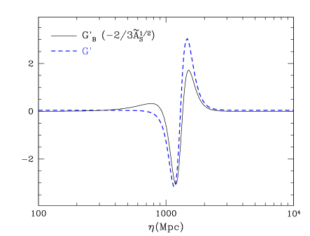
Figure 1: Bispectrum source GBsuperscriptsubscript𝐺𝐵G_{B}^{\prime} and power spectrum source Gsuperscript𝐺G^{\prime} in the GSR approximation for the step potential model (see §III.2). The bispectrum source has been rescaled by a constant related to A~S=2.39×10⁹subscript~𝐴𝑆2.39superscript109\tilde{A}_{S}=2.39\times 10^{-9} to eliminate its scaling with the power spectrum squared. Both sources share similar structure with features that integrate to zero as required for constant superhorizon behavior.

III.2 Step Potential

As an example, we consider the potential Adams et al. (2001)

V(ϕ)=12m2ϕ2[1+ctanh(ϕϕsd)],𝑉italic-ϕ12superscript𝑚2superscriptitalic-ϕ2delimited-[]1𝑐italic-ϕsubscriptitalic-ϕ𝑠𝑑\displaystyle V(\phi)=\frac{1}{2}m^{2}\phi^{2}\left[1+c\tanh\left(\frac{\phi-\phi_{s}}{d}\right)\right], (26)

which corresponds to a smooth step at ϕ=ϕsitalic-ϕsubscriptitalic-ϕ𝑠\phi=\phi_{s} of fractional height c𝑐c and width d𝑑d. Such a feature in the inflationary potential has been invoked to explain the ‘glitches’ in the CMB temperature anisotropy data at =20402040\ell=20-40 Covi et al. (2006); Hamann et al. (2007). Addressing the observability of the corresponding features in the bispectrum requires a fast approach to their calculation (see §IV).

For concreteness we adopt the WMAP5 maximum likelihood values of the parameters of the step potential Mortonson et al. (2009) {m,c,d,ϕs}={7.126×106,1.505×103,0.02705,14.668}𝑚𝑐𝑑subscriptitalic-ϕ𝑠7.126superscript1061.505superscript1030.0270514.668\{m,c,d,\phi_{s}\}=\{7.126\times 10^{-6},1.505\times 10^{-3},0.02705,14.668\}. We plot the bispectrum and power spectrum source functions for this model in Fig. 1. Note their similar structure once rescaled in amplitude. In Appendix B we consider an alternate choice of parameters to make contact with results in the literature.

Following the notation of the existing literature Chen et al. (2007, 2008), we construct plots related to

𝒢(k1,k2,k3)=k13k23k33(2π)4A~S2B(k1,k2,k3),𝒢subscript𝑘1subscript𝑘2subscript𝑘3superscriptsubscript𝑘13superscriptsubscript𝑘23superscriptsubscript𝑘33superscript2𝜋4superscriptsubscript~𝐴𝑆2subscript𝐵subscript𝑘1subscript𝑘2subscript𝑘3\displaystyle\mathcal{G}(k_{1},k_{2},k_{3})=\frac{k_{1}^{3}k_{2}^{3}k_{3}^{3}}{(2\pi)^{4}\tilde{A}_{S}^{2}}B_{{\cal R}}(k_{1},k_{2},k_{3}), (27)

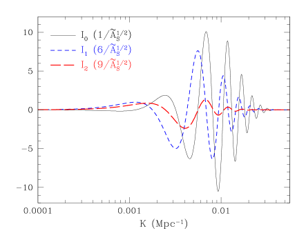
where A~Ssubscript~𝐴𝑆\tilde{A}_{S} is an arbitrary constant that is of order the curvature power spectrum normalization without the step feature. In practice we take A~S=2.39×10⁹subscript~𝐴𝑆2.39superscript109\tilde{A}_{S}=2.39\times 10^{-9}. Since 𝒢𝒢\mathcal{G} has dimensions of k3superscript𝑘3k^{3}, we typically divide it by some representative k3superscript𝑘3k^{3}. In Fig. 2 we show the one-dimensional GSR bispectrum integrals of Eq. (III.1) for this model. Note that I0(K)subscript𝐼0𝐾I_{0}(K) dominates, especially at high k𝑘k as discussed above.

Refer to caption

Figure 2: Bispectrum integrals in the zeroth-order GSR approximation for the step potential model as a function of the perimeter of the triangles K=k1+k2+k3𝐾subscript𝑘1subscript𝑘2subscript𝑘3K=k_{1}+k_{2}+k_{3}. All bispectrum triangles can be formed efficiently from these three integrals. Weights reflect how the integrals contribute to equilateral configurations. Note that I0subscript𝐼0I_{0} dominates the high k𝑘k structure.

III.3 Equilateral Limit

In the equilateral limit k1=k2=k3=keqsubscript𝑘1subscript𝑘2subscript𝑘3subscript𝑘eqk_{1}=k_{2}=k_{3}=k_{\rm eq} and Eqs. (21) and (27) simplify to

𝒢(keq,keq,keq)keq3𝒢subscript𝑘eqsubscript𝑘eqsubscript𝑘eqsuperscriptsubscript𝑘eq3\displaystyle\frac{\mathcal{G}(k_{\rm eq},k_{\rm eq},k_{\rm eq})}{k_{\rm eq}^{3}} =Δ3(keq)4A~S2[I06I1+9I2]K=3keq.absentsuperscriptsubscriptΔ3subscript𝑘eq4superscriptsubscript~𝐴𝑆2subscriptdelimited-[]subscript𝐼06subscript𝐼19subscript𝐼2𝐾3subscript𝑘eq\displaystyle={\Delta_{\cal R}^{3}(k_{\rm eq})\over 4\tilde{A}_{S}^{2}}\left[-I_{0}-6I_{1}+9I_{2}\right]_{K=3k_{\rm eq}}. (28)

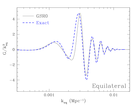
For equilateral triangles, the contribution from I0subscript𝐼0I_{0} dominates the result (see Fig. 2) and hence the comparison with the numerical evaluation of Eq. (II) tests this aspect of the GSR approximation (see Fig. 3). The zeroth-order GSR approximation captures the amplitude and phase of the oscillations fairly well. The largest deviations are at low k𝑘k for modes that were right on the horizon when the inflaton crossed the feature in Fig. 1. We show in Appendix A that these are associated with the neglect of first order terms involving other combinations of the real and imaginary parts of the mode functions.
Refer to caption

Figure 3: Zeroth-order GSR approximation for equilateral configurations in the step potential model compared with exact results of evaluating Eq. (II).

III.4 Squeezed Limit

For squeezed triangles kSk1k2k3kLsubscript𝑘𝑆subscript𝑘1much-less-thansubscript𝑘2subscript𝑘3subscript𝑘𝐿k_{S}\equiv k_{1}\ll k_{2}\approx k_{3}\equiv k_{L} and

𝒢(kS,kL,kL)kL3=𝒢subscript𝑘𝑆subscript𝑘𝐿subscript𝑘𝐿superscriptsubscript𝑘𝐿3absent\displaystyle\frac{\mathcal{G}(k_{S},k_{L},k_{L})}{k_{L}^{3}}= Δ(kS)Δ2(kL)4A~S2[2I1+4I2]K=2kL.subscriptΔsubscript𝑘𝑆subscriptsuperscriptΔ2subscript𝑘𝐿4superscriptsubscript~𝐴𝑆2subscriptdelimited-[]2subscript𝐼14subscript𝐼2𝐾2subscript𝑘𝐿\displaystyle{\Delta_{\cal R}(k_{S})\Delta^{2}_{\cal R}(k_{L})\over 4\tilde{A}_{S}^{2}}\left[-2I_{1}+4I_{2}\right]_{K=2k_{L}}. (29)

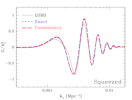
Note that in this limit only I1subscript𝐼1I_{1} and I2subscript𝐼2I_{2} contribute and hence the comparison in Fig. 4 tests a different aspect of the GSR approximation. In particular I1subscript𝐼1I_{1} and I2subscript𝐼2I_{2} carry the main impact of the source correction discussed below Eq. (III.1) since their windows carry superhorizon weight. In Appendix A, we use these triangle configurations to develop and test our approximation.

As a further check, it is well known that the bispectrum of curvature fluctuations produced by an inflationary model with a single ‘clock’ obeys a consistency relation which relates the squeezed limit of the bispectrum to the slope of the power spectrum Maldacena (2003). The squeezed limit corresponds to one of the curvature fluctuations in the bispectrum having a much longer wavelength than the remaining two kSkLmuch-less-thansubscript𝑘𝑆subscript𝑘𝐿k_{S}\ll k_{L}. In this limit, the consistency relation implies Creminelli and Zaldarriaga (2004)

𝒢(kS,kL,kL)kL3Δ2(kL)Δ2(kS)4A~S2dlnΔ2dlnk|kL.𝒢subscript𝑘𝑆subscript𝑘𝐿subscript𝑘𝐿superscriptsubscript𝑘𝐿3evaluated-atsuperscriptsubscriptΔ2subscript𝑘𝐿superscriptsubscriptΔ2subscript𝑘𝑆4superscriptsubscript~𝐴𝑆2𝑑superscriptsubscriptΔ2𝑑𝑘subscript𝑘𝐿\frac{\mathcal{G}(k_{S},k_{L},k_{L})}{k_{L}^{3}}\approx-{\Delta_{\cal R}^{2}(k_{L})\Delta_{\cal R}^{2}(k_{S})\over 4\tilde{A}_{S}^{2}}{d\ln\Delta_{\cal R}^{2}\over d\ln k}\Big{|}_{k_{L}}. (30)

In addition to the comparison of our approximation to the numerical results in this limit, we use the numerically computed local slope to test the consistency relation itself. The result is plotted in Fig. 4, which shows excellent agreement between the numerically computed bispectrum in the squeezed limit, and the result obtained from the slope of the power spectrum and the consistency relation. There are small discernible differences away from the effects of the feature; however, we attribute these to our truncation of the action at Eq. (II).
Refer to caption

Figure 4: Zeroth-order GSR approximation for squeezed bispectra k1=kSk2k3=kLsubscript𝑘1subscript𝑘𝑆much-less-thansubscript𝑘2subscript𝑘3subscript𝑘𝐿k_{1}=k_{S}\ll k_{2}\approx k_{3}=k_{L} in the step potential model compared with exact results of evaluating Eq. (II). Here kS=105subscript𝑘𝑆superscript105k_{S}=10^{-5} Mpc-1. For comparison the prediction from the consistency relation with the slope of the curvature power spectrum is also shown.

III.5 Flat Limit

Refer to caption

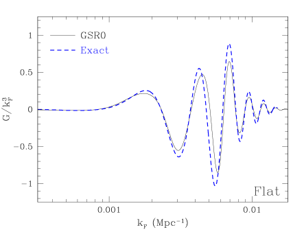
Figure 5: Zeroth-order GSR approximation for flat configurations with k1=kFsubscript𝑘1subscript𝑘𝐹k_{1}=k_{F} with k2=k3=kF/2subscript𝑘2subscript𝑘3subscript𝑘𝐹2k_{2}=k_{3}=k_{F}/2 in the step potential model compared with exact results of evaluating Eq. (II).

The final limit we consider is the flat limit, where kF=k1=2k2=2k3subscript𝑘𝐹subscript𝑘12subscript𝑘22subscript𝑘3k_{F}=k_{1}=2k_{2}=2k_{3} and the wavevectors are co-linear. Here

𝒢(kF,kF/2,kF/2)kF3𝒢subscript𝑘𝐹subscript𝑘𝐹2subscript𝑘𝐹2superscriptsubscript𝑘𝐹3\displaystyle\frac{\mathcal{G}(k_{F},k_{F}/2,k_{F}/2)}{k_{F}^{3}} =\displaystyle= Δ(kF)Δ2(kF/2)16A~S2subscriptΔsubscript𝑘𝐹subscriptsuperscriptΔ2subscript𝑘𝐹216superscriptsubscript~𝐴𝑆2\displaystyle{\Delta_{\cal R}(k_{F})\Delta^{2}_{\cal R}(k_{F}/2)\over 16\tilde{A}_{S}^{2}}
×[I07I1+12I2]K=2kF.absentsubscriptdelimited-[]subscript𝐼07subscript𝐼112subscript𝐼2𝐾2subscript𝑘𝐹\displaystyle\quad\times\left[-I_{0}-7I_{1}+12I_{2}\right]_{K=2k_{F}}.

and the approximation involves a combination of all three integrals. In Fig. 5, we show that the approximation works comparably well for flat triangles as equilateral and squeezed triangles.

IV CMB Signal-to-Noise

Given the step potential model that fits the glitches in the CMB power spectrum, the corresponding features in the bispectrum described in the previous section Covi et al. (2006); Hamann et al. (2007); Mortonson et al. (2009) are a firm prediction Chen et al. (2007, 2008). What is less clear is to what extent they are observable. Indeed that the model is designed to fit low multipole 2040similar-to2040\ell\sim 20-40 glitches in the power spectrum implies that these features will be strongly impacted by the cosmic variance of the dominant Gaussian fluctuations Chen et al. (2007). On the other hand, bispectrum features generically extend to higher k𝑘k and hence \ell than power spectra (see §III.1).

An estimate of the signal-to-noise in the bispectrum for the step potential has been hampered by the lack of a computationally efficient method for estimating the curvature bispectrum. Our zeroth-order GSR technique is ideal for these purposes as the bispectrum for any configuration can be simply formed from three precomputed integrals in Eq. (III.1).

IV.1 Cosmic Variance

The temperature or angular bispectrum is defined as the three-point function of the spherical harmonic coefficients amsubscript𝑎𝑚a_{\ell m} of the temperature anisotropy

B123=m1m2m3(123m1m2m3)a1m1a2m2a3m3.subscript𝐵subscript1subscript2subscript3subscriptsubscript𝑚1subscript𝑚2subscript𝑚3subscript1subscript2subscript3subscript𝑚1subscript𝑚2subscript𝑚3delimited-⟨⟩subscript𝑎subscript1subscript𝑚1subscript𝑎subscript2subscript𝑚2subscript𝑎subscript3subscript𝑚3B_{\ell_{1}\ell_{2}\ell_{3}}=\!\!\!\!\sum_{m_{1}m_{2}m_{3}}\left(\begin{array}[]{ccc}\ell_{1}&\ell_{2}&\ell_{3}\\ m_{1}&m_{2}&m_{3}\end{array}\right)\langle a_{\ell_{1}m_{1}}a_{\ell_{2}m_{2}}a_{\ell_{3}m_{3}}\rangle. (32)

The cosmic variance of the Gaussian part of the field puts an irreducible limit on the signal-to-noise ratio of

(SN)2=321B1232C1C2C3d123,superscript𝑆𝑁2subscriptsubscript3subscript2subscript1subscriptsuperscript𝐵2subscript1subscript2subscript3subscript𝐶subscript1subscript𝐶subscript2subscript𝐶subscript3subscript𝑑subscript1subscript2subscript3\left({S\over N}\right)^{2}=\sum_{\ell_{3}\geq\ell_{2}\geq\ell_{1}}{B^{2}_{\ell_{1}\ell_{2}\ell_{3}}\over C_{\ell_{1}}C_{\ell_{2}}C_{\ell_{3}}d_{\ell_{1}\ell_{2}\ell_{3}}}\,, (33)

where

d123=[1+δ12+δ23+δ31+2δ12δ23]subscript𝑑subscript1subscript2subscript3delimited-[]1subscript𝛿subscript1subscript2subscript𝛿subscript2subscript3subscript𝛿subscript3subscript12subscript𝛿subscript1subscript2subscript𝛿subscript2subscript3d_{\ell_{1}\ell_{2}\ell_{3}}=[1+\delta_{\ell_{1}\ell_{2}}+\delta_{\ell_{2}\ell_{3}}+\delta_{\ell_{3}\ell_{1}}+2\delta_{\ell_{1}\ell_{2}}\delta_{\ell_{2}\ell_{3}}] (34)

accounts for permuted contractions of repeated \ell’s and the angular power spectrum is defined by

amam=δδmmC.delimited-⟨⟩subscriptsuperscript𝑎𝑚subscript𝑎superscriptsuperscript𝑚subscript𝛿superscriptsubscript𝛿𝑚superscript𝑚subscript𝐶\langle a^{*}_{\ell m}a_{\ell^{\prime}m^{\prime}}\rangle=\delta_{\ell\ell^{\prime}}\delta_{mm^{\prime}}C_{\ell}\,. (35)

Thus to evaluate the signal-to-noise in the angular bispectrum we require not only a fast method for computing the curvature bispectrum but also for computing angular bispectra from curvature bispectra.

IV.2 Approximations

To obtain an order of magnitude estimate for the signal-to-noise ratio, we seek only a crude computation of the angular bispectrum from the curvature bispectrum. We therefore take the flat-sky approach and the Sachs-Wolfe limit for the temperature anisotropy.

In the flat-sky approximation, the angular bispectrum is defined by the three-point function of the Fourier moments of the temperature field given by a(𝐥)𝑎𝐥a({\bf l})

a(𝐥1)a(𝐥2)a(𝐥3)=(2π)2δ(𝐥1+𝐥2+𝐥3)B(1,2,3).delimited-⟨⟩𝑎subscript𝐥1𝑎subscript𝐥2𝑎subscript𝐥3superscript2𝜋2𝛿subscript𝐥1subscript𝐥2subscript𝐥3subscript𝐵subscript1subscript2subscript3\langle a({\bf l}_{1})a({\bf l}_{2})a({\bf l}_{3})\rangle=(2\pi)^{2}\delta({\bf l}_{1}+{\bf l}_{2}+{\bf l}_{3})B_{(\ell_{1},\ell_{2},\ell_{3})}. (36)

For 1subscript1\ell_{1}, 2subscript2\ell_{2}, 31much-greater-thansubscript31\ell_{3}\gg 1, it is related to the all-sky bispectra as Hu (2000)

B123subscript𝐵subscript1subscript2subscript3\displaystyle B_{\ell_{1}\ell_{2}\ell_{3}} =\displaystyle= (21+1)(22+1)(23+1)4π(123000)2subscript112subscript212subscript314𝜋subscript1subscript2subscript3000\displaystyle\sqrt{(2\ell_{1}+1)(2\ell_{2}+1)(2\ell_{3}+1)\over 4\pi}\left(\begin{array}[]{ccc}\ell_{1}&\ell_{2}&\ell_{3}\\ 0&0&0\end{array}\right) (40)
×B(1,2,3).absentsubscript𝐵subscript1subscript2subscript3\displaystyle\times B_{(\ell_{1},\ell_{2},\ell_{3})}.

Under the Sachs-Wolfe approximation, the temperature field as a function of angle 𝐧^^𝐧\hat{\bf n} on the sky is the projection of the curvature field onto the sphere at the recombination distance D𝐷D from the observer

a(𝐧^)=15(𝐱=D𝐧^)=15d3k(2π)3𝐤ei𝐤D𝐧^,𝑎^𝐧15𝐱𝐷^𝐧15superscript𝑑3𝑘superscript2𝜋3subscript𝐤superscript𝑒𝑖𝐤𝐷^𝐧a(\hat{\bf n})=-{1\over 5}{\cal R}({\bf x}=D{\hat{\bf n}})=-{1\over 5}\int{d^{3}k\over(2\pi)^{3}}{\cal R}_{\bf k}e^{i{\bf k}\cdot D{\hat{\bf n}}}, (41)

so that

B(1,2,3)subscript𝐵subscript1subscript2subscript3\displaystyle B_{(\ell_{1},\ell_{2},\ell_{3})} =\displaystyle= 253D40dk12πdk22π\displaystyle-{2\over 5^{3}D^{4}}\int_{0}^{\infty}{dk_{1\parallel}\over 2\pi}\int_{-\infty}^{\infty}{dk_{2\parallel}\over 2\pi} (42)
×B(k1,k2,k3)absentsubscript𝐵subscript𝑘1subscript𝑘2subscript𝑘3\displaystyle\times B_{{\cal R}}(k_{1},k_{2},k_{3})

where

𝐤1subscript𝐤1\displaystyle{\bf k}_{1} =\displaystyle= (𝐥1/D,k1),\displaystyle({\bf l}_{1}/D,k_{1\parallel}),
𝐤2subscript𝐤2\displaystyle{\bf k}_{2} =\displaystyle= (𝐥2/D,k2),\displaystyle({\bf l}_{2}/D,k_{2\parallel}),
𝐤3subscript𝐤3\displaystyle{\bf k}_{3} =\displaystyle= 𝐤1𝐤2,subscript𝐤1subscript𝐤2\displaystyle-{\bf k}_{1}-{\bf k}_{2}, (43)

and parallel-to\parallel is the direction along the line of sight, orthogonal to the plane of the sky. Note that even in this approximation, the signal-to-noise in the angular bispectrum is a five dimensional sum over the curvature bispectrum.

For consistency, we also compute Csubscript𝐶C_{\ell} under the same flat-sky, Sachs-Wolfe approximation for the cosmic variance in Eq. (33)

C=152D2dk2πP(𝐤=(𝐥/D,k)).subscript𝐶1superscript52superscript𝐷2𝑑subscript𝑘parallel-to2𝜋subscript𝑃𝐤𝐥𝐷subscript𝑘parallel-toC_{\ell}={1\over 5^{2}D^{2}}\int{dk_{\parallel}\over 2\pi}P_{\cal R}({\bf k}=({\bf l}/D,k_{\parallel})). (44)

In Fig. 6 we show the cumulative signal-to-noise as a function of the maximum \ell in the sum of Eq. (33) for the step model of §III.2. This model falls short of predicting observable effects by more than 104superscript10410^{4} in the number of bispectrum triangles or more than 102superscript10210^{2} in the amplitude of the bispectrum. Consequently, the crudeness of our curvature to angular bispectrum calculation is justified.

Refer to caption

Figure 6: Approximate cumulative signal-to-noise in the CMB angular bispectrum for the step model assuming cosmic variance limited temperature measurements out to a maximum multipole maxsubscriptmax\ell_{\rm max}. This model falls short of observable by more than 104superscript10410^{4} in the number of bispectrum triangles or 102superscript10210^{2} in the amplitude of the bispectrum.

V Discussion

We have developed a computationally efficient technique based on the generalized slow-roll approach for calculating the curvature bispectrum of models with features in the inflaton potential. This technique allows all configurations of the bispectrum to be calculated based on three precomputed integrals over the inflationary background reducing the dimensionality of the problem from three to one.

In this zeroth-order approximation, the accuracy is sufficient to capture the overall amplitude and structure of the bispectra to typically better than 20%. We have also developed a first order approximation that that brings the typical accuracy to better than several percent at the expense of raising the dimensionality to two.

The accuracy of the zeroth-order approximation more than suffices to make an estimate of the observability of the bispectrum features in the step potential model that best fits the WMAP power spectrum glitches at 2040similar-to2040\ell\sim 20-40. We find that the bispectrum amplitude is more that a factor of 100 too small to be observable in a cosmic variance limited measurement of CMB temperature anisotropy.

We have also explicitly verified that the consistency relation holds for a model of inflation which violates slow roll due to a sharp downward step feature in its potential. We find excellent agreement through the region affected by the feature, while small disparities at smaller and larger wavenumber are consistent with our neglect of additional terms suppressed by 𝒪(ϵH)𝒪subscriptitalic-ϵ𝐻\mathcal{O}(\epsilon_{H}) in the cubic action.

Two key general insights arise from the comparison of the GSR approach to the power spectrum and bispectrum. First, the dominant source of both is a similar combination of slow-roll parameters from the solution of the inflationary background. Second, the bispectrum is generated while modes were deeper within the horizon compared with the power spectrum.

The latter fact implies that features in the bispectrum generically persist to higher wavenumber k𝑘k than the power spectrum and provides a template for constructing models with large bispectrum features but small power spectrum features.

Indeed recent work has revealed an intriguing ‘decoupling’ limit under which large non-Gaussianity may be produced while the power spectrum remains largely unperturbed Flauger and Pajer (2011); Leblond and Pajer (2011). The application of the techniques we develop here may be able to extend the region of validity for these scenarios into the region where gravity is not completely decoupled, merely very weakly coupled. We defer these considerations to a future work.

Acknowledgements.
We thank Eugene Lim for providing numerical data for comparison. This work was supported in part by the Kavli Institute for Cosmological Physics at the University of Chicago through grants NSF PHY-0114422 and NSF PHY-0551142 and an endowment from the Kavli Foundation and its founder Fred Kavli. WH was additionally supported by U.S. Dept. of Energy contract DE-FG02-90ER-40560 and the David and Lucile Packard Foundation. HVP is supported by Marie Curie grant MIRG-CT-2007-203314 from the European Commission, and by STFC and the Leverhulme Trust, and acknowledges the hospitality of the KICP.

Appendix A Generalized Slow Roll

We begin in A.1 by reviewing the generalized slow-roll (GSR) formalism Stewart (2002); Choe et al. (2004); Dvorkin and Hu (2010), collecting some important results and establishing our notation. Employing the same methods used to correct the power spectrum in A.2, we derive the GSR expansion in for the bispectrum in A.3. We apply this expansion to the zeroth-order expansion used for the main results of the paper in A.4. This expression involves corrections for the superhorizon modes based on a more accurate first order approach that we develop and test in A.5.

The treatment and notations used here mirror the presentation in Dvorkin and Hu (2010). The reader is directed to these earlier works for further details. For notational compactness we express functions of the three separate bispectrum k𝑘k values as

F(ki)F(k1,k2,k3)𝐹subscript𝑘𝑖𝐹subscript𝑘1subscript𝑘2subscript𝑘3F(k_{i})\equiv F(k_{1},k_{2},k_{3}) (45)

throughout this Appendix.

A.1 GSR Corrections to the Mode Functions

Varying the action (1), the mode functions, k(η)subscript𝑘𝜂\mathcal{R}_{k}(\eta), satisfy the Mukhanov-Sasaki equation

d2kdx2(1ff)2xdkdx+k=0,superscript𝑑2subscript𝑘𝑑superscript𝑥21superscript𝑓𝑓2𝑥𝑑subscript𝑘𝑑𝑥subscript𝑘0\displaystyle\frac{d^{2}\mathcal{R}_{k}}{dx^{2}}-\left(1-{f^{\prime}\over f}\right)\frac{2}{x}\frac{d\mathcal{R}_{k}}{dx}+\mathcal{R}_{k}=0, (46)

where x=kη𝑥𝑘𝜂x=k\eta and f𝑓f were defined in Eq. (24).

We seek to expand the mode functions in a perturbative series around their infinitely slow-roll or de Sitter form. Since the comoving curvature ksubscript𝑘{\cal R}_{k} is undefined in that limit, it is useful to change variables to

yi=k32π2fxki.subscript𝑦𝑖superscript𝑘32superscript𝜋2𝑓𝑥subscriptsubscript𝑘𝑖y_{i}=\sqrt{k^{3}\over 2\pi^{2}}{f\over x}\mathcal{R}_{k_{i}}. (47)

This variable yisubscript𝑦𝑖y_{i} also carries the interpretation of the inflaton field fluctuation in the spatially flat gauge and is well defined in the de Sitter limit.

With this correspondence it is easy to see that well inside the horizon yisubscript𝑦𝑖y_{i} is more immune to features in the inflaton potential than ksubscript𝑘{\cal R}_{k} as it represents a free field. The converse is true outside the horizon. The latter is the primary flaw in GSR that we seek to rectify by enforcing constant curvature outside the horizon.

As an aside, note that similar superhorizon issues arise even for the computation of the bispectrum with the exact ksubscript𝑘{\cal R}_{k}. Although ksubscript𝑘{\cal R}_{k} does not respond significantly to the feature on such scales, ksuperscriptsubscript𝑘{\cal R}_{k}^{\prime} does and in such a way to exactly cancel the behavior in the ϵHsubscriptitalic-ϵ𝐻\epsilon_{H}, ηHsubscript𝜂𝐻\eta_{H} sources to keep the bispectrum constant in Eq. (II).

We then have

d2yidx2+(12x2)yi=g(lnη)x2yi,superscript𝑑2subscript𝑦𝑖𝑑superscript𝑥212superscript𝑥2subscript𝑦𝑖𝑔𝜂superscript𝑥2subscript𝑦𝑖\displaystyle\frac{d^{2}y_{i}}{dx^{2}}+\left(1-\frac{2}{x^{2}}\right)y_{i}=\frac{g(\ln\eta)}{x^{2}}y_{i}, (48)

where

g=f′′3ff,𝑔superscript𝑓′′3superscript𝑓𝑓\displaystyle g=\frac{f^{\prime\prime}-3f^{\prime}}{f}, (49)

and primes denote derivatives with respect to lnη𝜂\ln\eta.

The homogeneous Eq. (48) corresponds to exact de Sitter space (H=const.𝐻constH={\rm const.}) and has solutions

y0(x)=(1+ix)eix,subscript𝑦0𝑥1𝑖𝑥superscript𝑒𝑖𝑥\displaystyle y_{0}(x)=\left(1+\frac{i}{x}\right)e^{ix}, (50)

and y0(x)superscriptsubscript𝑦0𝑥y_{0}^{*}(x) which depend in the same way on x=kη𝑥𝑘𝜂x=k\eta for all k𝑘k. Given these solutions, we can use the Green function of the homogeneous operator to invert Eq. (48),

yi(x)=y0(x)+L(x,u)yi(u),subscript𝑦𝑖𝑥subscript𝑦0𝑥𝐿𝑥𝑢subscript𝑦𝑖𝑢\displaystyle y_{i}(x)=y_{0}(x)+L(x,u)y_{i}(u), (51)

with

L(x,u)yi(u)=xduu2g(lnη~)yi(u)[y0(u)y0(x)],𝐿𝑥𝑢subscript𝑦𝑖𝑢superscriptsubscript𝑥𝑑𝑢superscript𝑢2𝑔~𝜂subscript𝑦𝑖𝑢subscriptsuperscript𝑦0𝑢subscript𝑦0𝑥\displaystyle L(x,u)y_{i}(u)=-\int_{x}^{\infty}\frac{du}{u^{2}}g(\ln\tilde{\eta})y_{i}(u)\Im[y^{*}_{0}(u)y_{0}(x)], (52)

where u=kη~𝑢𝑘~𝜂u=k\tilde{\eta}. Note that unlike y0subscript𝑦0y_{0}, yisubscript𝑦𝑖y_{i} is not the same function of x=kη𝑥𝑘𝜂x=k\eta for all k𝑘k.

Then, assuming that the new solution is not too different from the de Sitter space result, we can employ the Born approximation and to solve the formal solution in Eq. (51) iteratively

yi(x)subscript𝑦𝑖𝑥\displaystyle y_{i}(x) =y0(x)+L(x,u)y0(u)+L(x,w)L(w,u)y0(u)+absentsubscript𝑦0𝑥𝐿𝑥𝑢subscript𝑦0𝑢𝐿𝑥𝑤𝐿𝑤𝑢subscript𝑦0𝑢\displaystyle=y_{0}(x)+L(x,u)y_{0}(u)+L(x,w)L(w,u)y_{0}(u)+\ldots (53)

We will also use the notation

W(u)=𝑊𝑢absent\displaystyle W(u)= 3u[y0(u)][y0(u)]3𝑢subscript𝑦0𝑢subscript𝑦0𝑢\displaystyle-\frac{3}{u}\Im[y_{0}(u)]\Re[y_{0}(u)]
=\displaystyle= 3sin(2u)2u33cos(2u)u23sin(2u)2u,32𝑢2superscript𝑢332𝑢superscript𝑢232𝑢2𝑢\displaystyle\frac{3\sin(2u)}{2u^{3}}-\frac{3\cos(2u)}{u^{2}}-\frac{3\sin(2u)}{2u},
X(u)=𝑋𝑢absent\displaystyle X(u)= 3u[y0(u)][y0(u)]3𝑢subscript𝑦0𝑢subscript𝑦0𝑢\displaystyle\frac{3}{u}\Re[y_{0}(u)]\Re[y_{0}(u)]
=\displaystyle= 3cos(2u)2u33sin(2u)u2+3cos(2u)2u32𝑢2superscript𝑢332𝑢superscript𝑢232𝑢2𝑢\displaystyle-\frac{3\cos(2u)}{2u^{3}}-\frac{3\sin(2u)}{u^{2}}+\frac{3\cos(2u)}{2u}
+32u3(1+u2),32superscript𝑢31superscript𝑢2\displaystyle+\frac{3}{2u^{3}}(1+u^{2}), (54)

and

[y0(u)][y0(u)]=1+1u2u3X(u).subscript𝑦0𝑢subscript𝑦0𝑢11superscript𝑢2𝑢3𝑋𝑢\displaystyle\Im[y_{0}(u)]\Im[y_{0}(u)]=1+\frac{1}{u^{2}}-\frac{u}{3}X(u). (55)

In the limit of small u𝑢u, these window functions behave as limu0W(u)=1subscript𝑢0𝑊𝑢1\lim_{u\rightarrow 0}W(u)=1 and limu0X(u)=u3/3subscript𝑢0𝑋𝑢superscript𝑢33\lim_{u\rightarrow 0}X(u)=u^{3}/3.

A.2 Power Spectrum Expansion

The curvature power spectrum is given by

Δ2(k)=limx1x2f2yi(x)yi(x).superscriptsubscriptΔ2𝑘subscriptmuch-less-than𝑥1superscript𝑥2superscript𝑓2subscript𝑦𝑖𝑥superscriptsubscript𝑦𝑖𝑥\displaystyle\Delta_{{\cal R}}^{2}(k)=\lim_{x\ll 1}\frac{x^{2}}{f^{2}}y_{i}(x)y_{i}^{*}(x)\,. (56)

At zeroth-order in the mode function correction and first order in g𝑔g we obtain Stewart (2002)

limx0(xyi)=subscript𝑥0𝑥subscript𝑦𝑖absent\displaystyle\lim_{x\rightarrow 0}(xy_{i})= ii3xduux3u3g(lnη)𝑖𝑖3superscriptsubscript𝑥𝑑𝑢𝑢superscript𝑥3superscript𝑢3𝑔𝜂\displaystyle i-\frac{i}{3}\int_{x}^{\infty}\frac{du}{u}\frac{x^{3}}{u^{3}}g(\ln\eta) (57)
+i3xduuW(u)g(lnη)𝑖3superscriptsubscript𝑥𝑑𝑢𝑢𝑊𝑢𝑔𝜂\displaystyle+\frac{i}{3}\int_{x}^{\infty}\frac{du}{u}W(u)g(\ln\eta)
13xduuX(u)g(lnη)+𝒪(x2),13superscriptsubscript𝑥𝑑𝑢𝑢𝑋𝑢𝑔𝜂𝒪superscript𝑥2\displaystyle-\frac{1}{3}\int_{x}^{\infty}\frac{du}{u}X(u)g(\ln\eta)+\mathcal{O}(x^{2}),

(which corrects a sign typo for the third term in Eq. (19) Dvorkin and Hu (2010)) where x=kη𝑥𝑘subscript𝜂x=k\eta_{*} and u=kη𝑢𝑘𝜂u=k\eta and so

Δ2(k)=1f2[1+23ff+13ηdηηW(kη)g(lnη)],superscriptsubscriptΔ2𝑘1superscript𝑓2delimited-[]123superscript𝑓𝑓13superscriptsubscriptsubscript𝜂𝑑𝜂𝜂𝑊𝑘𝜂𝑔𝜂\Delta_{{\cal R}}^{2}(k)={1\over f^{2}}\left[1+{2\over 3}{f^{\prime}\over f}+{1\over 3}\int_{\eta_{*}}^{\infty}{d\eta\over\eta}W(k\eta)g(\ln\eta)\right], (58)

since the X𝑋X term contributes quadratically.

The problem with this expression is that the power spectrum depends on the arbitrary end point of the integration ηsubscript𝜂\eta_{*}. The origin of this problem is that the curvature computed in the GSR approximation is not guaranteed to be constant outside the horizon and constancy is only enforced order by order in g𝑔g Dvorkin and Hu (2010). With large fluctuations, contributions that are formally higher order in g𝑔g supply necessary corrections.

To find these corrections, we can compute all of the first-order mode function corrections Choe et al. (2004) and retain the ones that contribute on superhorizon scales Dvorkin and Hu (2010)

lnΔGSR2(k)=G(lnη)+ηdηηW(kη)G(lnη),subscriptsuperscriptΔ2GSR𝑘𝐺subscript𝜂superscriptsubscriptsubscript𝜂𝑑𝜂𝜂𝑊𝑘𝜂superscript𝐺𝜂\displaystyle\ln\Delta^{2}_{\rm GSR}(k)=G(\ln\eta_{*})+\int_{\eta_{*}}^{\infty}\frac{d\eta}{\eta}W(k\eta)G^{\prime}(\ln\eta), (59)

where the modified source is

G(lnη)=23(gf2f2).superscript𝐺𝜂23𝑔superscript𝑓2superscript𝑓2\displaystyle G^{\prime}(\ln\eta)=\frac{2}{3}\left(g-{f^{\prime 2}\over f^{2}}\right). (60)

Formally Gsuperscript𝐺G^{\prime} involves a first-order correction to the source since f/f=𝒪(g)superscript𝑓𝑓𝒪𝑔f^{\prime}/f={\cal O}(g). Note that for superhorizon modes when the inflaton crosses the feature W(kη)1𝑊𝑘𝜂1W(k\eta)\rightarrow 1 and the power spectrum no longer depends on the arbitrary end point.

We will follow this procedure to define our zeroth-order bispectrum formulation in Eq. (21).

A.3 Bispectrum Expansion

In terms of the above notation, the bispectrum in Eq. (II) takes the form

B(ki)subscript𝐵subscript𝑘𝑖\displaystyle B_{\mathcal{R}}(k_{i}) =(2π)4η34k1k2k3f3{iy1(k1η)y2(k2η)y3(k3η)\displaystyle=\frac{(2\pi)^{4}\eta_{*}^{3}}{4k_{1}k_{2}k_{3}f^{3}}\Re\Big{\{}iy_{1}(k_{1}\eta_{*})y_{2}(k_{2}\eta_{*})y_{3}(k_{3}\eta_{*})
ηdηηgB(lnη)Dη[y1(k1η)y2(k2η)y3(k3η)]}\displaystyle\int^{\infty}_{\eta_{*}}\frac{d\eta}{\eta}g_{B}(\ln\eta)D_{\eta}[y_{1}^{*}(k_{1}\eta)y_{2}^{*}(k_{2}\eta)y_{3}^{*}(k_{3}\eta)]\Big{\}}
+BoundaryTerms,BoundaryTerms\displaystyle+{\rm Boundary\;\;Terms}, (61)

and the differential operator

Dη=ddlnη+3(1ff).subscript𝐷𝜂𝑑𝑑𝜂31superscript𝑓𝑓D_{\eta}=\frac{d}{d\ln\eta}+3\left(1-\frac{f^{\prime}}{f}\right). (62)

In the Eq. (A.3), “Boundary Terms” refers to the second term in Eq. (II). While these terms are physically important, they represent a small correction and we defer their discussion to a subsection.

Here the unmodified source function, which we will subsequently modify in a similar prescription to g3G/2𝑔3superscript𝐺2g\rightarrow 3G^{\prime}/2, is

gB(lnη)=(ϵHηH)f.subscript𝑔𝐵𝜂superscriptsubscriptitalic-ϵ𝐻subscript𝜂𝐻𝑓\displaystyle g_{B}(\ln\eta)=\frac{(\epsilon_{H}-\eta_{H})^{\prime}}{f}. (63)

By analogy to the power spectrum window functions, let us define the window functions

WB(xi)subscript𝑊𝐵subscript𝑥𝑖\displaystyle W_{B}(x_{i}) [y1(x1)y2(x2)y3(x3)],absentsubscript𝑦1subscript𝑥1subscript𝑦2subscript𝑥2subscript𝑦3subscript𝑥3\displaystyle\equiv\Re[y_{1}(x_{1})y_{2}(x_{2})y_{3}(x_{3})],
XB(xi)subscript𝑋𝐵subscript𝑥𝑖\displaystyle X_{B}(x_{i}) [y1(x1)y2(x2)y3(x3)].absentsubscript𝑦1subscript𝑥1subscript𝑦2subscript𝑥2subscript𝑦3subscript𝑥3\displaystyle\equiv\Im[y_{1}(x_{1})y_{2}(x_{2})y_{3}(x_{3})]. (64)

For the zeroth-order mode functions, yiy0subscript𝑦𝑖subscript𝑦0y_{i}\rightarrow y_{0}, WBWB0subscript𝑊𝐵superscriptsubscript𝑊𝐵0W_{B}\rightarrow W_{B}^{0}, XBXB0subscript𝑋𝐵superscriptsubscript𝑋𝐵0X_{B}\rightarrow X_{B}^{0}

WB0(xi)superscriptsubscript𝑊𝐵0subscript𝑥𝑖\displaystyle W_{B}^{0}(x_{i}) =\displaystyle= 1x1x2x3[(X+x1x2x3)cosX\displaystyle{1\over x_{1}x_{2}x_{3}}\Big{[}(-X+x_{1}x_{2}x_{3})\cos X
+(1x2x3x1x2x1x3)sinX],\displaystyle\quad+(1-x_{2}x_{3}-x_{1}x_{2}-x_{1}x_{3})\sin X\Big{]},
XB0(xi)superscriptsubscript𝑋𝐵0subscript𝑥𝑖\displaystyle X_{B}^{0}(x_{i}) =\displaystyle= 1x1x2x3[(1x2x3x1x2x1x3)cosX\displaystyle-{1\over x_{1}x_{2}x_{3}}\Big{[}(1-x_{2}x_{3}-x_{1}x_{2}-x_{1}x_{3})\cos X (65)
+(Xx1x2x3)sinX],\displaystyle\quad+(X-x_{1}x_{2}x_{3})\sin X\Big{]},

where X=x1+x2+x3𝑋subscript𝑥1subscript𝑥2subscript𝑥3X=x_{1}+x_{2}+x_{3}, and is not to be confused with the window function X(kη)𝑋𝑘𝜂X(k\eta). Note that the trigonometric functions depend only on the perimeter of the triangle K𝐾K and that the prefactors are pure powers of kisubscript𝑘𝑖k_{i}. This is a critical simplification achieved by using zeroth-order mode functions.

As we shall see, their superhorizon limit will be particularly important

limki0WB0(kiη)=subscriptsubscript𝑘𝑖0subscriptsuperscript𝑊0𝐵subscript𝑘𝑖𝜂absent\displaystyle\lim_{k_{i}\rightarrow 0}W^{0}_{B}(k_{i}\eta)= k13+k23+k333k1k2k3+𝒪(ki2η2),superscriptsubscript𝑘13superscriptsubscript𝑘23superscriptsubscript𝑘333subscript𝑘1subscript𝑘2subscript𝑘3𝒪superscriptsubscript𝑘𝑖2superscript𝜂2\displaystyle\frac{k_{1}^{3}+k_{2}^{3}+k_{3}^{3}}{3k_{1}k_{2}k_{3}}+\mathcal{O}(k_{i}^{2}\eta^{2}), (66)
limki0XB0(kiη)=subscriptsubscript𝑘𝑖0subscriptsuperscript𝑋0𝐵subscript𝑘𝑖𝜂absent\displaystyle\lim_{k_{i}\rightarrow 0}X^{0}_{B}(k_{i}\eta)= 1k1k2k3η3+12k12+k22+k32k1k2k3η+𝒪(kiη).1subscript𝑘1subscript𝑘2subscript𝑘3superscript𝜂312superscriptsubscript𝑘12superscriptsubscript𝑘22superscriptsubscript𝑘32subscript𝑘1subscript𝑘2subscript𝑘3𝜂𝒪subscript𝑘𝑖𝜂\displaystyle-\frac{1}{k_{1}k_{2}k_{3}\eta^{3}}+\frac{1}{2}\frac{k_{1}^{2}+k_{2}^{2}+k_{3}^{2}}{k_{1}k_{2}k_{3}\eta}+\mathcal{O}(k_{i}\eta).

To an arbitrary order, the bispectrum can be written

B(ki)subscript𝐵subscript𝑘𝑖\displaystyle B_{\mathcal{R}}(k_{i}) (2π)44k1k2k3η3f3{i[WB(kiη)+iXB(kiη)]\displaystyle\approx\frac{(2\pi)^{4}}{4k_{1}k_{2}k_{3}}\frac{\eta_{*}^{3}}{f^{3}}\Re\Big{\{}i[W_{B}(k_{i}\eta_{*})+iX_{B}(k_{i}\eta_{*})]
×ηdηηgB(lnη)Dη[WB(kiη)iXB(kiη)]}.\displaystyle\quad\times\int^{\infty}_{\eta_{*}}\frac{d\eta}{\eta}g_{B}(\ln\eta)D_{\eta}\left[W_{B}(k_{i}\eta)-iX_{B}(k_{i}\eta)\right]\Big{\}}. (67)

Specifically, using this notation we can write the zeroth and first-order bispectrum as

B(ki)subscript𝐵subscript𝑘𝑖\displaystyle B_{\mathcal{R}}(k_{i}) (2π)44k1k2k3η3f3ηdηηgB(lnη)Dη{\displaystyle\approx\frac{(2\pi)^{4}}{4k_{1}k_{2}k_{3}}\frac{\eta_{*}^{3}}{f^{3}}\int^{\infty}_{\eta_{*}}\frac{d\eta}{\eta}g_{B}(\ln\eta)D_{\eta}\big{\{} (68)
WB0(kiη)XB0(kiη)(1[𝒞(ki,η)𝒞(ki,η)])subscriptsuperscript𝑊0𝐵subscript𝑘𝑖subscript𝜂subscriptsuperscript𝑋0𝐵subscript𝑘𝑖𝜂1𝒞subscript𝑘𝑖𝜂𝒞subscript𝑘𝑖subscript𝜂\displaystyle\quad W^{0}_{B}(k_{i}\eta_{*})X^{0}_{B}(k_{i}\eta)(1-\Re[\mathcal{C}(k_{i},\eta)-\mathcal{C}(k_{i},\eta_{*})])
XB0(kiη)WB0(kiη)(1[𝒞(ki,η)𝒞(ki,η)])subscriptsuperscript𝑋0𝐵subscript𝑘𝑖subscript𝜂subscriptsuperscript𝑊0𝐵subscript𝑘𝑖𝜂1𝒞subscript𝑘𝑖𝜂𝒞subscript𝑘𝑖subscript𝜂\displaystyle-X^{0}_{B}(k_{i}\eta_{*})W^{0}_{B}(k_{i}\eta)(1-\Re[\mathcal{C}(k_{i},\eta)-\mathcal{C}(k_{i},\eta_{*})])
+WB0(kiη)WB0(kiη)[𝒞(ki,η)𝒞(ki,η)]subscriptsuperscript𝑊0𝐵subscript𝑘𝑖subscript𝜂subscriptsuperscript𝑊0𝐵subscript𝑘𝑖𝜂𝒞subscript𝑘𝑖subscript𝜂𝒞subscript𝑘𝑖𝜂\displaystyle+W^{0}_{B}(k_{i}\eta_{*})W^{0}_{B}(k_{i}\eta)\,\Im[\mathcal{C}(k_{i},\eta_{*})-\mathcal{C}(k_{i},\eta)]
+XB0(kiη)XB0(kiη)[𝒞(ki,η)𝒞(ki,η)]},\displaystyle+X^{0}_{B}(k_{i}\eta_{*})X^{0}_{B}(k_{i}\eta)\,\Im[\mathcal{C}(k_{i},\eta_{*})-\mathcal{C}(k_{i},\eta)]\big{\}},

where

𝒞(ki,η)=j=13ηdη~η~g(lnη~)kjη~y0(kjη~)y0(kjη)[y0(kjη~)y0(kjη)].𝒞subscript𝑘𝑖𝜂superscriptsubscript𝑗13subscriptsuperscript𝜂𝑑~𝜂~𝜂𝑔~𝜂subscript𝑘𝑗~𝜂subscript𝑦0subscript𝑘𝑗~𝜂subscript𝑦0subscript𝑘𝑗𝜂subscriptsuperscript𝑦0subscript𝑘𝑗~𝜂subscript𝑦0subscript𝑘𝑗𝜂\displaystyle\mathcal{C}(k_{i},\eta)=\sum_{j=1}^{3}\int^{\infty}_{\eta}{d\tilde{\eta}\over\tilde{\eta}}\frac{g(\ln\tilde{\eta})}{k_{j}\tilde{\eta}}\frac{y_{0}(k_{j}\tilde{\eta})}{y_{0}(k_{j}\eta)}\Im[y^{*}_{0}(k_{j}\tilde{\eta})y_{0}(k_{j}\eta)]. (69)

The fact that 𝒞𝒞\mathcal{C} depends on the three k𝑘k’s presents the main obstacle to simplifying the first-order expressions.
Refer to caption

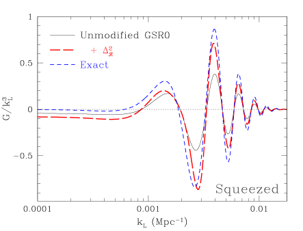
Figure 7: Unmodified source with zeroth-order GSR approximation for squeezed triangles as in Fig. 4. Solid lines denote unmodified form (70). Red dashed lines represent the replacement of the external 1/f1𝑓1/f with ΔsubscriptΔ\Delta_{\cal R} in Eq. (72). Here η=1subscript𝜂1\eta_{*}=1Mpc.

A.4 Zeroth-Order Bispectrum

We define the order of our approximation by whether the mode functions used in the construction are the zeroth-order de Sitter y0subscript𝑦0y_{0} or an iterative expansion. Thus we allow ourselves the freedom to add higher order corrections to the source function but not the mode function. This operational definition, rather than order counting in g𝑔g is motivated by simple form of the bispectrum that results. With only zeroth-order mode functions, all triangles can be expressed in terms of single integrals that depend only on the perimeter of the triangle.

A.4.1 Unmodified Source

We begin with the zeroth-order approximation using the original source gBsubscript𝑔𝐵g_{B} in Eq. (63). This form is consistently first order in the deviations from slow roll and of the terms in Eq. (68) only the XB0(kiη)WB0(kiη)superscriptsubscript𝑋𝐵0subscript𝑘𝑖subscript𝜂superscriptsubscript𝑊𝐵0subscript𝑘𝑖𝜂X_{B}^{0}(k_{i}\eta_{*})W_{B}^{0}(k_{i}\eta) leading order term survives

B(ki)subscript𝐵subscript𝑘𝑖\displaystyle\!\!\!\!\!\!\!B_{{\cal R}}(k_{i}) (2π)44k12k22k321f3[ηdηηgB(lnη)(WB0+3WB0)].\displaystyle\approx{(2\pi)^{4}\over 4k_{1}^{2}k_{2}^{2}k_{3}^{2}}{1\over f^{3}}\Big{[}\int^{\infty}_{\eta_{*}}\frac{d\eta}{\eta}g_{B}(\ln\eta)(W_{B}^{0}{}^{\prime}+3W_{B}^{0})\Big{]}. (70)

In Fig. 7, we compare this approximation with the exact result for squeezed triangles. There are two obvious flaws in this expression. First the external f=f(lnη)𝑓𝑓subscript𝜂f=f(\ln\eta_{*}) factors depend on the arbitrary end point. Second, in the superhorizon limit WB0superscriptsubscript𝑊𝐵0W_{B}^{0} goes to a constant defined in Eq. (66). Thus, analogous to the behavior of the power spectrum in the same approximation, the feature is imprinted on superhorizon modes.

A.4.2 Source Modification

Just as in the power spectrum case, we can fix these problems by examining the first-order mode function corrections in the superhorizon limit. We start from the full first-order expression Eq. (68) and extract a factor of

1[𝒞(ki,η)]=1+ff+jηdηηg(lnη)3W(kjη),1𝒞subscript𝑘𝑖subscript𝜂1superscript𝑓𝑓subscript𝑗subscriptsuperscriptsubscript𝜂𝑑𝜂𝜂𝑔𝜂3𝑊subscript𝑘𝑗𝜂1-\Re[\mathcal{C}(k_{i},\eta_{*})]=1+\frac{f^{\prime}}{f}+\sum_{j}\int^{\infty}_{\eta_{*}}\frac{d\eta}{\eta}{g(\ln\eta)\over 3}W(k_{j}\eta), (71)

where we have evaluated the expression in the limit kiη1much-less-thansubscript𝑘𝑖subscript𝜂1k_{i}\eta_{*}\ll 1. We have also dropped higher order terms.

Combined with the factors of 1/f1𝑓1/f we recognize these factors as the GSR expression (58) for the power spectrum. Our prescription therefore is to replace these terms with the exact power spectrum

1f3(1[𝒞(ki,η)])=Δ(k1)Δ(k2)Δ(k3).1superscript𝑓31𝒞subscript𝑘𝑖subscript𝜂subscriptΔsubscript𝑘1subscriptΔsubscript𝑘2subscriptΔsubscript𝑘3\displaystyle\frac{1}{f^{3}}(1-\Re[\mathcal{C}(k_{i},\eta_{*})])=\Delta_{\cal R}(k_{1})\Delta_{\cal R}(k_{2})\Delta_{\cal R}(k_{3}). (72)

This fixes the problem of the external f𝑓f factors in Eq. (70). In Fig. 7, we show the impact of applying this correction. The low k𝑘k features in particular are modulated and enhanced by the external power spectra but the superhorizon problem remains.

We then look at the superhorizon limit of the rest of the first-order corrections. Since WBsubscript𝑊𝐵W_{B} scales as a constant in the superhorizon limit, we need only keep the constant parts of the expansion of [𝒞(ki,η)]𝒞subscript𝑘𝑖𝜂\Re[\mathcal{C}(k_{i},\eta)]

limki0[𝒞(ki,η)]subscriptsubscript𝑘𝑖0𝒞subscript𝑘𝑖𝜂\displaystyle\lim_{k_{i}\rightarrow 0}\Re[\mathcal{C}(k_{i},\eta)] =j=13[13xjdη~η~η3η~3g(lnη~)\displaystyle=\sum_{j=1}^{3}\Big{[}\frac{1}{3}\int_{x_{j}}^{\infty}\frac{d\tilde{\eta}}{\tilde{\eta}}\frac{\eta^{3}}{\tilde{\eta}^{3}}g(\ln\tilde{\eta}) (73)
13xjdη~η~W(kjη~)g(lnη~)+𝒪(kj2η2)].\displaystyle-\frac{1}{3}\int_{x_{j}}^{\infty}\frac{d\tilde{\eta}}{\tilde{\eta}}W(k_{j}\tilde{\eta})g(\ln\tilde{\eta})+\mathcal{O}(k_{j}^{2}\eta^{2})\Big{]}.

On the other hand, XBsubscript𝑋𝐵X_{B} behaves as ki3superscriptsubscript𝑘𝑖3k_{i}^{-3}, so we need to keep up to 𝒪(ki3)𝒪superscriptsubscript𝑘𝑖3{\cal O}(k_{i}^{3}) parts of [𝒞(ki,η)]𝒞subscript𝑘𝑖𝜂\Im[\mathcal{C}(k_{i},\eta)]:

limki0[𝒞(ki,η)]subscriptsubscript𝑘𝑖0𝒞subscript𝑘𝑖𝜂\displaystyle\!\!\lim_{k_{i}\rightarrow 0}\Im[\mathcal{C}(k_{i},\eta)] =\displaystyle= j=13[13ηdη~η~X(kjη~)g(lnη~)\displaystyle\sum_{j=1}^{3}\Big{[}-\frac{1}{3}\int_{\eta}^{\infty}\frac{d\tilde{\eta}}{\tilde{\eta}}X(k_{j}\tilde{\eta})g(\ln\tilde{\eta}) (74)
+2(kjη)39ηdη~η~W(kjη~)g(lnη~)2superscriptsubscript𝑘𝑗𝜂39superscriptsubscript𝜂𝑑~𝜂~𝜂𝑊subscript𝑘𝑗~𝜂𝑔~𝜂\displaystyle+\frac{2(k_{j}\eta)^{3}}{9}\int_{\eta}^{\infty}\frac{d\tilde{\eta}}{\tilde{\eta}}W(k_{j}\tilde{\eta})g(\ln\tilde{\eta})
(kjη)39ηdη~η~η3η~3g(lnη~)superscriptsubscript𝑘𝑗𝜂39superscriptsubscript𝜂𝑑~𝜂~𝜂superscript𝜂3superscript~𝜂3𝑔~𝜂\displaystyle-\frac{(k_{j}\eta)^{3}}{9}\int_{\eta}^{\infty}\frac{d\tilde{\eta}}{\tilde{\eta}}\frac{\eta^{3}}{\tilde{\eta}^{3}}g(\ln\tilde{\eta})
+𝒪(kj5η2η~3)].\displaystyle+\mathcal{O}(k_{j}^{5}\eta^{2}\tilde{\eta}^{3})\Big{]}.

Then, working to order 𝒪(gBf/f)𝒪subscript𝑔𝐵superscript𝑓𝑓\mathcal{O}(g_{B}{f^{\prime}}/{f})

B(ki)subscript𝐵subscript𝑘𝑖\displaystyle B_{\mathcal{R}}(k_{i}) 3(2π)44k12k22k32Δ(k1)Δ(k2)Δ(k3)k13+k23+k333k1k2k3absent3superscript2𝜋44superscriptsubscript𝑘12superscriptsubscript𝑘22superscriptsubscript𝑘32subscriptΔsubscript𝑘1subscriptΔsubscript𝑘2subscriptΔsubscript𝑘3superscriptsubscript𝑘13superscriptsubscript𝑘23superscriptsubscript𝑘333subscript𝑘1subscript𝑘2subscript𝑘3\displaystyle\approx{3(2\pi)^{4}\over 4k_{1}^{2}k_{2}^{2}k_{3}^{2}}\Delta_{\cal R}(k_{1})\Delta_{\cal R}(k_{2})\Delta_{\cal R}(k_{3})\frac{k_{1}^{3}+k_{2}^{3}+k_{3}^{3}}{3k_{1}k_{2}k_{3}}
×ηdηηgB[1ηdη~η~ff].\displaystyle\quad\times\int^{\infty}_{\eta_{*}}\frac{d\eta}{\eta}g_{B}\Bigg{[}1-\int^{\infty}_{\eta}\frac{d\tilde{\eta}}{\tilde{\eta}}\frac{f^{\prime}}{f}\Bigg{]}. (75)

Now, to a good approximation,

gB=(ϵHηH)f1f(ff).subscript𝑔𝐵superscriptsubscriptitalic-ϵ𝐻subscript𝜂𝐻𝑓1𝑓superscriptsuperscript𝑓𝑓\displaystyle g_{B}=\frac{(\epsilon_{H}-\eta_{H})^{\prime}}{f}\approx-\frac{1}{f}\left(\frac{f^{\prime}}{f}\right)^{\prime}. (76)

With this approximation for the source, integrating the second line of Eq. (A.4.2) by parts one obtains

ηdηη(1fff)1fffηdηηff.subscriptsuperscriptsubscript𝜂𝑑𝜂𝜂superscript1𝑓superscript𝑓𝑓1𝑓superscript𝑓𝑓subscriptsuperscriptsubscript𝜂𝑑𝜂𝜂superscript𝑓𝑓\displaystyle-\int^{\infty}_{\eta_{*}}\frac{d\eta}{\eta}\left(\frac{1}{f}\frac{f^{\prime}}{f}\right)^{\prime}-\frac{1}{f}\frac{f^{\prime}}{f}\int^{\infty}_{\eta_{*}}\frac{d\eta}{\eta}\frac{f^{\prime}}{f}. (77)

Dropping the slow-roll suppressed second term, we can account for this first-order effect on superhorizon scales by the replacement

gB1f(ff)(1fff)(ϵHηHf)GB.subscript𝑔𝐵1𝑓superscriptsuperscript𝑓𝑓superscript1𝑓superscript𝑓𝑓superscriptsubscriptitalic-ϵ𝐻subscript𝜂𝐻𝑓superscriptsubscript𝐺𝐵\displaystyle g_{B}\approx-\frac{1}{f}\left(\frac{f^{\prime}}{f}\right)^{\prime}\rightarrow-\left(\frac{1}{f}\frac{f^{\prime}}{f}\right)^{\prime}\approx\left(\frac{\epsilon_{H}-\eta_{H}}{f}\right)^{\prime}\equiv G_{B}^{\prime}. (78)

In the superhorizon limit, the contribution of the first term in Eq. (II) to the bispectrum then reduces to the integral of a total derivative of slow-roll parameters, which are small at late times, once the inflaton has settled back onto the slow-roll attractor.

To summarize, our zeroth-order approximation consists of the replacement of the source by Eq. (78) and the replacement of the external factors using Eq. (72) while using the de Sitter mode functions everywhere else. These replacements lead to the expression in Eq. (21) with the help of the explicit form for the WB0superscriptsubscript𝑊𝐵0W_{B}^{0} window in Eq. (65). In particular note that the I0subscript𝐼0I_{0} term arises from the WB0W_{B}^{0}{}^{\prime} term in Eq. (70).

A.4.3 Boundary Terms

While small, the boundary term in Eq. (II) hitherto omitted plays an important role in ensuring that the bispectrum becomes independent of time on superhorizon scales.

The contribution from the boundary term can be obtained from the results of the previous section with the replacement

ηdηηgB(lnη)(ϵHηH)f|η=η,subscriptsuperscriptsubscript𝜂𝑑𝜂𝜂subscript𝑔𝐵𝜂evaluated-atsubscriptitalic-ϵ𝐻subscript𝜂𝐻𝑓𝜂subscript𝜂\displaystyle\int^{\infty}_{\eta_{*}}\frac{d\eta}{\eta}g_{B}(\ln\eta)\rightarrow\left.\frac{(\epsilon_{H}-\eta_{H})}{f}\right|_{\eta=\eta_{*}}, (79)

together the replacement of all η𝜂\eta by ηsubscript𝜂\eta_{*}. Using this replacement on Eq. (A.4.2) yields for the boundary term

BBT(ki)subscriptsuperscript𝐵BTsubscript𝑘𝑖\displaystyle B^{\rm BT}_{\mathcal{R}}(k_{i}) =3(2π)44k12k22k32Δ(k1)Δ(k2)Δ(k3)k13+k23+k333k1k2k3absent3superscript2𝜋44superscriptsubscript𝑘12superscriptsubscript𝑘22superscriptsubscript𝑘32subscriptΔsubscript𝑘1subscriptΔsubscript𝑘2subscriptΔsubscript𝑘3superscriptsubscript𝑘13superscriptsubscript𝑘23superscriptsubscript𝑘333subscript𝑘1subscript𝑘2subscript𝑘3\displaystyle={3(2\pi)^{4}\over 4k_{1}^{2}k_{2}^{2}k_{3}^{2}}\Delta_{\cal R}(k_{1})\Delta_{\cal R}(k_{2})\Delta_{\cal R}(k_{3})\frac{k_{1}^{3}+k_{2}^{3}+k_{3}^{3}}{3k_{1}k_{2}k_{3}}
×(ϵHηHf)[1ηdηηff].absentsubscriptitalic-ϵ𝐻subscript𝜂𝐻𝑓delimited-[]1subscriptsuperscriptsubscript𝜂𝑑𝜂𝜂superscript𝑓𝑓\displaystyle\quad\times\left(\frac{\epsilon_{H}-\eta_{H}}{f}\right)\Bigg{[}1-\int^{\infty}_{\eta_{*}}\frac{d{\eta}}{\eta}\frac{f^{\prime}}{f}\Bigg{]}. (80)

Notice that, when added to Eq. (A.4.2) using Eq. (77), one obtains perfect cancellation leaving a time independent result. Since the integral term in Eq. (A.4.3) exactly cancels the second term in (77) we choose to omit both in practice. This brings the net boundary term to the GB(lnη)subscript𝐺𝐵subscript𝜂G_{B}(\ln\eta_{*}) contribution to Eq. (21).

We also point out here that, while for convenience we have evaluated our expressions at a time when the inflaton has passed the feature and is back on its slow-roll attractor, our results are not restricted to this regime. As we pointed out in Section II, the cancellation we are enforcing is exact and thus truly independent of the time at which the bispectrum is evaluated, even if this time is chosen to be when the slow-roll parameters are not small.

A.5 First-Order Bispectrum

We can further compute to first order in the mode function correction on all scales. Note that the first order corrections represent a calculation of the bispectrum to second order in the slow-roll parameters. Additionally, note that the boundary terms are always suppressed by slow-roll parameters evaluated at times well after the inflaton has traversed the feature which means that they are computationally irrelevant.

Neglecting boundary terms we obtain at first order in the GSR approximation, the full bispectrum

B(ki)=subscript𝐵subscript𝑘𝑖absent\displaystyle B_{{\cal R}}(k_{i})= (2π)44ΔGSR(k1)k12ΔGSR(ki)k22ΔGSR(k3)k32superscript2𝜋44subscriptΔGSRsubscript𝑘1superscriptsubscript𝑘12subscriptΔGSRsubscript𝑘𝑖superscriptsubscript𝑘22subscriptΔGSRsubscript𝑘3superscriptsubscript𝑘32\displaystyle{(2\pi)^{4}\over 4}{\Delta_{\rm GSR}(k_{1})\over k_{1}^{2}}{\Delta_{\rm GSR}(k_{i})\over k_{2}^{2}}{\Delta_{\rm GSR}(k_{3})\over k_{3}^{2}}
×ηdηηgB(lnη)[U0+U1A+U1B+U1C\displaystyle\times\int^{\infty}_{\eta_{*}}{d\eta\over\eta}g_{B}(\ln\eta)[U_{0}+U_{1A}+U_{1B}+U_{1C}
+U1D+U1E](kiη),\displaystyle\qquad+U_{1D}+U_{1E}](k_{i}\eta), (81)

where

U0(kiη)=subscript𝑈0subscript𝑘𝑖𝜂absent\displaystyle U_{0}(k_{i}\eta)= (ddlnη+3)[y0(k1η)y0(k2η)y0(k3η)],𝑑𝑑𝜂3subscript𝑦0subscript𝑘1𝜂subscript𝑦0subscript𝑘2𝜂subscript𝑦0subscript𝑘3𝜂\displaystyle\left(\frac{d}{d\ln\eta}+3\right)\Re[y_{0}(k_{1}\eta)y_{0}(k_{2}\eta)y_{0}(k_{3}\eta)],
U1A(kiη)=subscript𝑈1𝐴subscript𝑘𝑖𝜂absent\displaystyle U_{1A}(k_{i}\eta)= 12ηdη~η~G(lnη~)X(k3η~)(ddlnη+3)12superscriptsubscriptsubscript𝜂𝑑~𝜂~𝜂superscript𝐺~𝜂𝑋subscript𝑘3~𝜂𝑑𝑑𝜂3\displaystyle{1\over 2}\int_{\eta_{*}}^{\infty}{d\tilde{\eta}\over\tilde{\eta}}G^{\prime}(\ln\tilde{\eta})X(k_{3}\tilde{\eta})\left(\frac{d}{d\ln\eta}+3\right)
×[y0(k1η)y0(k2η)[y0(k3η)+y0(k3η)]]absentsubscript𝑦0subscript𝑘1𝜂subscript𝑦0subscript𝑘2𝜂delimited-[]subscriptsuperscript𝑦0subscript𝑘3𝜂subscript𝑦0subscript𝑘3𝜂\displaystyle\times\Im[y_{0}(k_{1}\eta)y_{0}(k_{2}\eta)[y^{*}_{0}(k_{3}\eta)+y_{0}(k_{3}\eta)]]
+cyc.,cyc\displaystyle\qquad+{\rm cyc.},
U1B(kiη)=subscript𝑈1𝐵subscript𝑘𝑖𝜂absent\displaystyle U_{1B}(k_{i}\eta)= 12ηdη~η~G(lnη~)W(k3η~)12superscriptsubscript𝜂𝑑~𝜂~𝜂superscript𝐺~𝜂𝑊subscript𝑘3~𝜂\displaystyle-{1\over 2}\int_{\eta}^{\infty}{d\tilde{\eta}\over\tilde{\eta}}G^{\prime}(\ln\tilde{\eta})W(k_{3}\tilde{\eta})
×(ddlnη+3)[y0(k1η)y0(k2η)y0(k3η)]absent𝑑𝑑𝜂3subscript𝑦0subscript𝑘1𝜂subscript𝑦0subscript𝑘2𝜂subscriptsuperscript𝑦0subscript𝑘3𝜂\displaystyle\times\left(\frac{d}{d\ln\eta}+3\right)\Re[y_{0}(k_{1}\eta)y_{0}(k_{2}\eta)y^{*}_{0}(k_{3}\eta)]
+cyc.,cyc\displaystyle\quad+{\rm cyc.},
U1C(kiη)=subscript𝑈1𝐶subscript𝑘𝑖𝜂absent\displaystyle U_{1C}(k_{i}\eta)= 12ηηdη~η~G(lnη~)X(k3η~)12superscriptsubscriptsubscript𝜂𝜂𝑑~𝜂~𝜂superscript𝐺~𝜂𝑋subscript𝑘3~𝜂\displaystyle-{1\over 2}\int_{\eta_{*}}^{\eta}{d\tilde{\eta}\over\tilde{\eta}}G^{\prime}(\ln\tilde{\eta})X(k_{3}\tilde{\eta})
×(ddlnη+3)[y0(k1η)y0(k2η)y0(k3η)]absent𝑑𝑑𝜂3subscript𝑦0subscript𝑘1𝜂subscript𝑦0subscript𝑘2𝜂subscriptsuperscript𝑦0subscript𝑘3𝜂\displaystyle\times\left(\frac{d}{d\ln\eta}+3\right)\Im[y_{0}(k_{1}\eta)y_{0}(k_{2}\eta)y^{*}_{0}(k_{3}\eta)]
+cyc.,cyc\displaystyle+{\rm cyc.},
U1D(kiη)=subscript𝑈1𝐷subscript𝑘𝑖𝜂absent\displaystyle U_{1D}(k_{i}\eta)= 34ηdη~η~G(lnη~)(1k3η~+1(k3η~)3)34superscriptsubscript𝜂𝑑~𝜂~𝜂superscript𝐺~𝜂1subscript𝑘3~𝜂1superscriptsubscript𝑘3~𝜂3\displaystyle-{3\over 4}\int_{\eta}^{\infty}{d\tilde{\eta}\over\tilde{\eta}}G^{\prime}(\ln\tilde{\eta})\left({1\over k_{3}\tilde{\eta}}+{1\over(k_{3}\tilde{\eta})^{3}}\right)
(ddlnη+3)[y0(k1η)y0(k2η)\displaystyle\left(\frac{d}{d\ln\eta}+3\right)\Im[y_{0}(k_{1}\eta)y_{0}(k_{2}\eta)
[y0(k3η)+y0(k3η)]]+cyc.,\displaystyle[y^{*}_{0}(k_{3}\eta)+y_{0}(k_{3}\eta)]]+{\rm cyc.},
U1E(kiη)=subscript𝑈1𝐸subscript𝑘𝑖𝜂absent\displaystyle U_{1E}(k_{i}\eta)= 3[y0(k1η)y0(k2η)y0(k3η)]3subscript𝑦0subscript𝑘1𝜂subscript𝑦0subscript𝑘2𝜂subscript𝑦0subscript𝑘3𝜂\displaystyle-3\Re[y_{0}(k_{1}\eta)y_{0}(k_{2}\eta)y_{0}(k_{3}\eta)]
×ff[112gB(ff)2],absentsuperscript𝑓𝑓delimited-[]112subscript𝑔𝐵superscriptsuperscript𝑓𝑓2\displaystyle\times{f^{\prime}\over f}\left[1-{1\over 2g_{B}}\left({f^{\prime}\over f}\right)^{2}\right], (82)

where cyc. denotes the 2 additional cyclic permutations of the k𝑘k indices.

In order to fix a small second order correction to the superhorizon results we have replaced g3G/2𝑔3superscript𝐺2g\rightarrow 3G^{\prime}/2 in the the first order expressions and likewise replace the source term

ffff[112gB(ff)2]superscript𝑓𝑓superscript𝑓𝑓delimited-[]112subscript𝑔𝐵superscriptsuperscript𝑓𝑓2{f^{\prime}\over f}\rightarrow{f^{\prime}\over f}\left[1-{1\over 2g_{B}}\left({f^{\prime}\over f}\right)^{2}\right] (83)

in U1Esubscript𝑈1𝐸U_{1E}. Furthermore for consistency, we use the GSR power spectrum approximation (59) for the external terms.
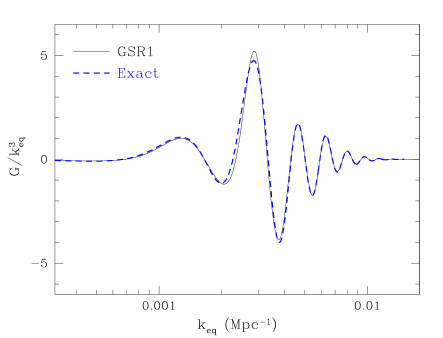
Refer to caption

Figure 8: First order GSR mode function approximation for the step model compared with the exact solution.

For the case of the equilateral configurations, this expression simplifies considerably and are practical to evaluate

B(k,k,k)subscript𝐵𝑘𝑘𝑘\displaystyle B_{{\cal R}}(k,k,k) =(2π)4ΔGSR3(k)4k6ηdηηgB(lnη)[U0eq\displaystyle={(2\pi)^{4}\Delta_{\rm GSR}^{3}(k)\over 4k^{6}}\int_{\eta_{*}}^{\infty}{d\eta\over\eta}g_{B}(\ln\eta)[U_{0}^{\rm eq}
+U1Aeq+U1Beq+U1Ceq+U1Deq+U1Eeq](kη),\displaystyle\quad+U_{1A}^{\rm eq}+U_{1B}^{\rm eq}+U_{1C}^{\rm eq}+U_{1D}^{\rm eq}+U_{1E}^{\rm eq}](k\eta), (84)

where

U0eq(v)superscriptsubscript𝑈0eq𝑣\displaystyle U_{0}^{\rm eq}(v) =\displaystyle= 6cos3v+3(1v2)sin3vv,63𝑣31superscript𝑣23𝑣𝑣\displaystyle-6\cos 3v+{3(1-v^{2})\sin 3v\over v},
U1Aeq(v)superscriptsubscript𝑈1𝐴eq𝑣\displaystyle U_{1A}^{\rm eq}(v) =\displaystyle= 32v[(3+v2)cosv+3(v21)cos3v\displaystyle{3\over 2v}\big{[}(3+v^{2})\cos v+3(v^{2}-1)\cos 3v
+2v(sinv3sin3v)]\displaystyle\quad+2v(\sin v-3\sin 3v)\big{]}
×ηdη~η~G(lnη~)X(kη~),\displaystyle\times\int_{\eta_{*}}^{\infty}{d\tilde{\eta}\over\tilde{\eta}}G^{\prime}(\ln\tilde{\eta})X(k\tilde{\eta}),
U1Beq(v)superscriptsubscript𝑈1𝐵eq𝑣\displaystyle U_{1B}^{\rm eq}(v) =\displaystyle= 32[(3+v2)sinvv2cosv]32delimited-[]3superscript𝑣2𝑣𝑣2𝑣\displaystyle{3\over 2}\left[{(3+v^{2})\sin v\over v}-2\cos v\right]
×ηdη~η~G(lnη~)W(kη~),\displaystyle\quad\times\int_{\eta}^{\infty}{d\tilde{\eta}\over\tilde{\eta}}G^{\prime}(\ln\tilde{\eta})W(k\tilde{\eta}),
U1Ceq(v)superscriptsubscript𝑈1𝐶eq𝑣\displaystyle U_{1C}^{\rm eq}(v) =\displaystyle= 32[(3v+v)cosv+2sinv]32delimited-[]3𝑣𝑣𝑣2𝑣\displaystyle-{3\over 2}\left[\left({3\over v}+v\right)\cos v+2\sin v\right]
×ηηdη~η~G(lnη~)X(kη~),\displaystyle\quad\times\int_{\eta_{*}}^{\eta}{d\tilde{\eta}\over\tilde{\eta}}G^{\prime}(\ln\tilde{\eta})X(k\tilde{\eta}),
U1Deq(v)superscriptsubscript𝑈1𝐷eq𝑣\displaystyle U_{1D}^{\rm eq}(v) =\displaystyle= 94v[(3+v2)cosv+3(v21)cos3v\displaystyle-{9\over 4v}\big{[}(3+v^{2})\cos v+3(v^{2}-1)\cos 3v
+2v(sinv3sin3v)]\displaystyle\quad+2v(\sin v-3\sin 3v)\big{]}
×ηdη~η~G(lnη~)(1v~+1v~3),\displaystyle\quad\times\int_{\eta}^{\infty}{d\tilde{\eta}\over\tilde{\eta}}G^{\prime}(\ln\tilde{\eta})\left({1\over\tilde{v}}+{1\over\tilde{v}^{3}}\right),
U1Eeq(v)superscriptsubscript𝑈1𝐸eq𝑣\displaystyle U_{1E}^{\rm eq}(v) =\displaystyle= 3v3[v(v23)cos3v+(13v2)sin3v]3superscript𝑣3delimited-[]𝑣superscript𝑣233𝑣13superscript𝑣23𝑣\displaystyle-{3\over v^{3}}\left[v(v^{2}-3)\cos 3v+(1-3v^{2})\sin 3v\right] (85)
×ff[112gB(ff)2].absentsuperscript𝑓𝑓delimited-[]112subscript𝑔𝐵superscriptsuperscript𝑓𝑓2\displaystyle\quad\times{f^{\prime}\over f}\left[1-{1\over 2g_{B}}\left({f^{\prime}\over f}\right)^{2}\right].

We show the result of computing these terms for the step model of §III.2 in Fig. 8. Note that most of the error in the zeroth-order approximation is corrected by the first order expression. The dominant correction is from U1Aeqsuperscriptsubscript𝑈1𝐴eqU_{1A}^{\rm eq} and involves the product of two independent integrals. Since its computation is no more intensive than the zeroth-order expression, it may be simultaneously computed as a monitor of the accuracy of the zeroth-order expression. Note that the integral of GXsuperscript𝐺𝑋G^{\prime}X is the same as the one that monitors the accuracy of the power spectrum approximation Dvorkin and Hu (2010).
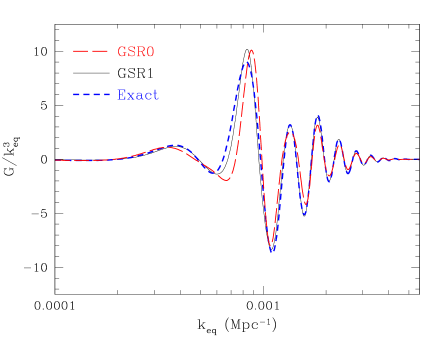
Refer to caption

Figure 9: Bispectrum in the step model of Ref. Chen et al. (2007, 2008) and A~S=4.415×10¹⁰subscript~𝐴𝑆4.415superscript1010\tilde{A}_{S}=4.415\times 10^{-10} (see text). Our approximations work equally well for models with larger bispectrum features.

This first order mode function correction breaks the property that all triangles depend only on integrals involving the perimeter K𝐾K. Thus though more accurate it is of more limited utility for fast computations in that the six integrals involved are a function of two variables: the perimeter K𝐾K and the wavenumber of the corrected mode function k3subscript𝑘3k_{3}. Nonetheless it still reduces the complexity of the exact computation which requires all three kisubscript𝑘𝑖k_{i} as well as the exact mode functions for each individual kisubscript𝑘𝑖k_{i}.

Appendix B Comparison to Previous Work

Previous calculations of the step bispectrum employed the parameters of: {m,c,d,ϕs}={3×106,1.8×103,0.022,14.84}𝑚𝑐𝑑subscriptitalic-ϕ𝑠3superscript1061.8superscript1030.02214.84\{m,c,d,\phi_{s}\}=\{3\times 10^{-6},1.8\times 10^{-3},0.022,14.84\} Chen et al. (2007, 2008). There are three important differences between this model and the one defined in §III.2.

First due to an error in the setting of the initial conditions in Ref. Covi et al. (2006); Hamann et al. (2007) the location of the feature ϕssubscriptitalic-ϕ𝑠\phi_{s} is shifted and the corresponding features in the power spectrum and bispectrum appear at lower k𝑘k. Secondly, the maximum likelihood fit to WMAP5 data prefer a slightly larger width d𝑑d compared with WMAP3 data. Since the bispectrum is particularly sensitive to the width d𝑑d, its features appear more prominent and persist to higher k𝑘k. Finally Ref. Chen et al. (2007, 2008) arbitrarily set the parameter m𝑚m whereas Ref. Covi et al. (2006); Hamann et al. (2007) normalized to WMAP3. As a consequence, we take A~S=4.415×10¹⁰subscript~𝐴𝑆4.415superscript1010\tilde{A}_{S}=4.415\times 10^{-10} to be compatible with this choice.

In Fig. 9 we show our zeroth-order, first-order and exact calculation of this model. We have verified that the exact calculation accurately reproduces the results in Ref. Chen et al. (2007).

References