Capacity to within 3 bits for a class of Gaussian Interference Channels with a Cognitive Relay

Abstract

The InterFerence Channel with a Cognitive Relay (IFC-CR) consists of a classical two-user interference channel in which the two independent messages are also non-causally known at a cognitive relay node. In this work a special class of IFC-CRs in which the sources do not create interference at the non-intended destinations is analyzed. This special model results in a channel with two non-interfering point-to-point channels whose transmission is aided by an in-band cognitive relay, which is thus referred to as the Parallel Channel with a Cognitive Relay (PC-CR). We determine the capacity of the PC-CR channel to within 3 bits/s/Hz for all channel parameters. In particular, we present several new outer bounds which we achieve to within a constant gap by proper selection of Gaussian input distributions in a simple rate-splitting and superposition coding-based inner bound. The inner and outer bounds are numerically evaluated to show that the actual gap can be far less than 3 bits/s/Hz.

I Introduction

The concepts of interference, cognition – or non-causal message knowledge at a subset of network nodes – and relaying have all been of great recent interest. While capacities of the interference, cognitive and relay channels remain open for the general discrete memoryless channel models, they are known for certain classes of channels, and known to within constant gaps for the Gaussian noise counterparts. In this work we focus on a particular channel model which illustrates the power of cognition and simultaneous relaying which we term the Parallel Channel with a Cognitive Relay (PC-CR), which encompasses several multi-user and cognitive/cooperative channel models, such as the Broadcast Channel (BC) and the Cognitive InterFerence Channel (CIFC).

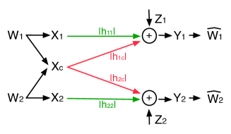
The PC-CR is a sub-channel of the more general interference channel with a cognitive relay (IFC-CR). The IFC-CR consists of a classical two-user interference channel in which the two independent messages, each known at the corresponding source node, are also non-causally known at a third, in-band transmitter node, which we term the cognitive relay. This five-node channel generalizes a number of known channels including the BC, the IFC, and the CIFC. The PC-CR consists of an IFC-CR in which the two sources do not interfere at the non-intended destinations (see Fig. 1) thus resulting into two parallel point-to-point channels whose communication is aided by a single cognitive relay which knows both messages non-causally. As such, the emphasis is placed on the transmission strategy of the single cognitive relay: it may choose to help one source, the other, or both and it is this tradeoff that the PC-CR seeks to characterize.

Figure 1: The GPC-CR channel with two messages $W_{1}$ and $W_{2}$ known non-causally at the Cognitive Relay (CR).

Past Work. The PC-CR has not been explicitly considered aside from the authors’ previous work [1], where an outer bound for the general discrete memoryless IFC-CR was presented and then tightened for certain deterministic channels. We then demonstrated that this outer bound is capacity for the high-SNR linear deterministic approximation of the Gaussian PC-CR. In this work, we go beyond our previous work in [1] by considering the Gaussian PC-CR model for finite SNR.

More generally, as the PC-CR is a subset of the IFC-CR, the literature for the latter channel is of direct relevance. The IFC with a relay was first introduced in [2] and [3], where the message knowledge at the relay was obtained causally and non-causally, respectively. Here we focus on the non-causal version of the problem [3], also termed the “broadcast channel with cognitive relays” [4], and thus we omit the body of work related to the causal (i.e., non-cognitive) relay model. In [3], dirty-paper coding, beamforming and interference reduction techniques are combined in the derivation of an achievable rate region for the Gaussian single-input single-output (SISO) IFC-CR. In [5], the achievable region of [3] is further improved upon and a sum-rate outer bound based on the MIMO Gaussian C-IFC is proposed. In [4], an achievable rate region that contains all previously known regions is proposed.

Contributions and Paper Organization. In this work we study the Gaussian PC-CR (GPC-CR). We expand upon the limited prior work on the PC-CR, never explicitly considered in Gaussian noise, by:

$\bullet$ specializing the outer bound in [1] to the GPC-CR (Section III-A) and deriving two new outer bounds (Section III-B),

$\bullet$ specializing the achievable scheme in [6] to the GPC-CR (Section IV),

$\bullet$ determining capacity to within 3 bits/s/Hz by selecting Gaussian inputs in the achievable scheme that mimic the capacity achieving scheme of the corresponding high-SNR linear deterministic approximation channel [1] (Section V),

$\bullet$ numerically evaluating inner and outer bounds, which indicate an even small than 3 bits/s/Hz gap (Section V).

Section VI concludes the paper.

II Channel Model

We use definitions and notation as in [7], and let $\mathcal{C}(x)\triangleq\log_{2}(1+x)$, and $\bar{\alpha}\triangleq 1-\alpha$ for $\alpha\ \in\ [0,1]$. A complex-valued GPC-CR in standard form is a five-node network (see Fig. 1) with inputs ($X_{1},X_{2},X_{c}$) and outputs ($Y_{1},Y_{2}$) related through:

$$Y_{1} =|h_{11}|X_{1}+|h_{1c}|X_{c}+Z_{1},$$ (1a)

$$Y_{2} =|h_{22}|X_{2}+|h_{2c}|X_{c}+Z_{2},$$ (1b)

where $Z_{i}\sim\mathcal{N}(0,1)$ and where the inputs are subject to a power constraint $\mathbb{E}[|X_{i}|^{2}]\leq 1$, $i=\{1,2,c\}$. The channel links $h_{i}$, $i\in\{11,22,1c,2c\}$ can be taken to be real-valued without loss of generality because receivers and transmitters can compensate for the phase of the output signals. The correlation among the noises is irrelevant because the capacity of the channel without receiver cooperation only depends on the noise marginal distributions [8].

A rate-pair $(R_{1},R_{2})$ is achievable if there exist a sequence of encoding functions over $N$ channel uses $X_{i}^{N}=X_{i}^{N}(W_{i})$, $i\in\{1,2\}$, and $X_{c}^{N}=X_{c}^{N}(W_{1},W_{2})$ (where we note the non-causal message knowledge at the relay), for messages $W_{1}$ and $W_{2}$ independent and uniformly distributed on $[1:2^{NR_{1}}]$ and $[1:2^{NR_{2}}]$, respectively, and a sequence of decoding functions $\widehat{W}_{i}=\widehat{W}_{i}(Y_{i}^{N})$, $i\in\{1,2\},$ such that $\mathop{\mathrm{missing}}{Pr}\nolimits\left[\widehat{W}_{i}\neq W_{i}\right]\to 0$ as $N\to\infty$ for $i\in\{1,2\}$. The capacity region is the convex closure of the set of achievable $(R_{1},R_{2})$-pairs.

III Outer Bounds

In this section we derive a series of outer bounds to the capacity region of the GPC-CR. Our first outer bound is obtained by evaluating the outer bound we derived in [1, Th. III.1] for a general memoryless IFC-CR (which, as in Sato’s outer bound for the BC [8], exploits the fact that the capacity region only depends on the conditional marginal distributions of the channel) for the GPC-CR model. The resulting outer bound is the tightest known for the GPC-CR but it is expressed as a function of four correlation parameters, which make its analytical manipulation difficult. For this reason, we then proceed to derive a simpler (expression-wise) piecewise linear approximation of our first outer bound that will be used to derive the constant gap result in the “large SNR” regime. Then, by following the approach of [9, Th. III.7], we derive other two outer bounds by transforming the GPC-CR into a channel for which tight bounds are available. These two bounds will be used in the derivation of the constant gap results in the “small SNR” regime.

III-A Tightest known outer bound

Theorem 1.

The capacity of a GPC-CR is contained in the region:

$$R_{1} \leq\mathcal{C}(|h_{11}|^{2}+|h_{1c}|^{2}(1-|\rho_{2c}|^{2})+2\mathrm{Re}\{\rho_{1c}\}|h_{1c}||h_{11}|),$$ (2a)

$$R_{2} \leq\mathcal{C}(|h_{22}|^{2}+|h_{2c}|^{2}(1-|\rho_{1c}|^{2})+2\mathrm{Re}\{\rho_{2c}\}|h_{2c}||h_{22}|),$$ (2b)

$$R_{1}+R_{2} \leq\mathcal{C}(|h_{22}|^{2}+|h_{2c}|^{2}+2\mathrm{Re}\{\rho_{2c}\}|h_{2c}||h_{22}|)+\min_{\rho_{z}:|\rho_{z}|\leq 1}$$

$$\mathcal{C}\left(|h_{11}|^{2}+\frac{|h_{1c}|^{2}}{|h_{2c}|^{2}}-2\frac{\mathrm{Re}\{\rho_{z}\}|h_{1c}|}{|h_{2c}|}-\frac{\left|\rho_{1c}|h_{11}||h_{2c}|+\rho_{z}-\frac{|h_{1c}|}{|h_{2c}|}\right|^{2}}{|h_{2c}|^{2}(1-|\rho_{2c}|^{2})+1}\right)$$

$$-\log(1-|\rho_{z}|^{2})$$ (2c)

$$R_{1}+R_{2} \leq\mathcal{C}(|h_{11}|^{2}+|h_{1c}|^{2}+2\mathrm{Re}\{\rho_{1c}\}|h_{1c}||h_{11}|)+\min_{\rho_{z}:|\rho_{z}|\leq 1}$$

$$\mathcal{C}\left(|h_{22}|^{2}+\frac{|h_{2c}|^{2}}{|h_{1c}|^{2}}-2\frac{\mathrm{Re}\{\rho_{z}\}|h_{2c}|}{|h_{1c}|}-\frac{\left|\rho_{2c}|h_{22}||h_{1c}|+\rho_{z}-\frac{|h_{2c}|}{|h_{1c}|}\right|^{2}}{|h_{1c}|^{2}(1-|\rho_{1c}|^{2})+1}\right)$$

$$-\log(1-|\rho_{z}|^{2})$$ (2d)

for all $(|\rho_{1c}|,|\rho_{2c}|)\in[0,1]^{2}$ such that $|\rho_{1c}|^{2}+|\rho_{2c}|^{2}\leq 1$.

Proof:

Consider the outer bound in [1, Th. III.1] for a general IFC-CR, given by:

$$R_{1} \leq I(Y_{1};X_{1},X_{c}|X_{2},Q),$$

$$R_{2} \leq I(Y_{2};X_{2},X_{c}|X_{1},Q),$$

$$R_{1}+R_{2} \leq I(Y_{2};X_{1},X_{2},X_{c},Q)+I(Y_{1};X_{1},X_{c}|Y_{2},X_{2},Q)$$

$$R_{1}+R_{2} \leq I(Y_{1};X_{1},X_{2},X_{c},Q)+I(Y_{2};X_{2},X_{c}|Y_{1},X_{1},Q),$$

for some input distribution that factors as $P_{Q,X_{1},X_{2},X_{c}}=P_{Q}P_{X_{1}|Q}P_{X_{2}|Q}P_{X_{c}|X_{1},X_{2},Q}$. By specializing the above bound to the GPC-CR, the “Gaussian maximizes entropy” theorem [7] guarantees that the following Gaussian input:

$$\begin{pmatrix}X_{1}\\ X_{2}\\ X_{c}\\ \end{pmatrix}\sim\mathcal{N}\left(\bm{0},\begin{pmatrix}1&0&\rho_{1c}\\ 0&1&\rho_{2c}\\ \rho_{1c}^{*}&\rho_{2c}^{*}&1\\ \end{pmatrix}\right)$$ (3)

exhausts the outer region (because every mutual information term contains all the inputs). The covariance matrix in (3) is positive semi-definite if and only if $|\rho_{1c}|^{2}+|\rho_{2c}|^{2}\leq 1$. Evaluating the outer bound region for the jointly Gaussian input in (3) yields the region in (2). The minimization over $\rho_{z}=\mathbb{E}[Z_{1}Z_{2}^{*}]$ in each of the sum-rate bounds is possible because the joint conditional distribution can be chosen so as to tighten the bound. ∎

Given that our outer bound in Th. 1 is expressed as the union over all feasible correlation coefficients that satisfy $|\rho_{1c}|^{2}+|\rho_{2c}|^{2}=1$, it is not immediately useful in the derivation of the constant gap result. To address this, we loosen the outer bound in Th. 1 and in doing so obtain a new, simpler piecewise linear outer bound expression, which will be used in constant gap result in Section V.

Theorem 2.

Piecewise linear outer bound. The region in Th. 1 is included into:

$$R_{1} \leq\mathcal{C}(\max\{|h_{11}|^{2},|h_{1c}|^{2}\})+\log(4),$$ (4a)

$$R_{2} \leq\mathcal{C}(\max\{|h_{22}|^{2},|h_{2c}|^{2}\})+\log(4),$$ (4b)

$$R_{1}+R_{2} \leq\mathcal{C}(\max\{|h_{22}|^{2},|h_{2c}|^{2}\})$$

$$+\mathcal{C}\left(\max\left\{|h_{11}|^{2},\frac{|h_{1c}|^{2}}{|h_{2c}|^{2}}\right\}\right)+\log(8),$$ (4c)

$$R_{1}+R_{2} \leq\mathcal{C}(\max\{|h_{11}|^{2},|h_{1c}|^{2}\})$$

$$+\mathcal{C}\left(\max\left\{|h_{22}|^{2},\frac{|h_{2c}|^{2}}{|h_{1c}|^{2}}\right\}\right)+\log(8).$$ (4d)

Proof:

For the $R_{1}$-bound (and similarly for $R_{2}$-bound):

$$R_{1} \leq\mathcal{C}\left(|h_{11}|^{2}+|h_{1c}|^{2}(1-|\rho_{2c}|^{2})+2\mathrm{Re}\{\rho_{1c}\}|h_{1c}||h_{11}|\right)$$

$$\leq\mathcal{C}\left((|h_{11}|+|h_{1c}|)^{2}\}\right)\leq\mathcal{C}\left(4\max\{|h_{11}|^{2},|h_{1c}|^{2}\}\right)$$

$$\leq\mathcal{C}(\max\{|h_{11}|^{2},|h_{1c}|^{2}\})+\log(4).$$

For the sum-rate bounds we let $\rho_{z}=0$ and we proceed as for the $R_{1}$-bound. Note that our gap of 3 bits/s/Hz will come form the term $\log(8)=3~{}$ bits in (4c) and (4d) . ∎

III-B Outer bounds by transformation

We now present two additional outer bounds that are obtained by transforming the GPC-CR in the spirit of [10, Th. II.7]. In particular, we show that the capacity of the PC-CR is contained into: 1) the capacity region of a cognitive IFC and a point-to-point (P2P) channel in parallel, and 2) the capacity region of two P2P channels and a BC channel all in parallel. The proofs can be found in the Appendix and basically follows by showing that independent coding across the transformed parallel channels is optimal.

Theorem 3.

CIFC+P2P outer bound. The capacity of the GPC-CR is contained into the outer bound to the capacity region of the channel in Fig. 3 given by:

$$R_{1} \leq\mathcal{C}\left(\frac{\alpha|h_{1c}|^{2}}{1-\sigma_{11}^{2}}\right)+\mathcal{C}\left(\frac{|h_{11}|^{2}}{\sigma_{11}^{2}}\right),$$ (5a)

$$R_{1}+R_{2} \leq\mathcal{C}\left(\bar{\alpha}|h_{2c}|^{2}+|h_{22}|^{2}+2\sqrt{\bar{\alpha}}|h_{2c}||h_{22}|\right)$$ (5b)

$$+ \left[\mathcal{C}\left(\frac{\alpha|h_{1c}|^{2}}{1-\sigma_{11}^{2}}\right)-\mathcal{C}\left(\alpha|h_{2c}|^{2}\right)\right]^{+}+\mathcal{C}\left(\frac{|h_{11}|^{2}}{\sigma_{11}^{2}}\right),$$ (5c)

taken over the union of all $\alpha\in[0,1]$, for any $\sigma_{11}^{2}\leq 1$.

Theorem 4.

Parallel P2P+BC outer bound. The capacity of the GPC-CR is contained into the capacity region of the channel in Fig. 3 given by:

$$R_{1} \leq\mathcal{C}\left(\frac{\bar{\alpha}|h_{1c}|^{2}}{1-\sigma_{11}^{2}}\right)+\mathcal{C}\left(\frac{|h_{11}|^{2}}{\sigma_{11}^{2}}\right),$$ (6a)

$$R_{2} \leq\mathcal{C}\left(\frac{\alpha|h_{2c}|^{2}}{\bar{\alpha}|h_{2c}|^{2}+1-\sigma_{22}^{2}}\right)+\mathcal{C}\left(\frac{|h_{22}|^{2}}{\sigma_{22}^{2}}\right),$$ (6b)

union over all $\alpha\in[0,1]$, for any $\sigma^{2}_{1},\sigma^{2}_{2}\leq 1$ such that

$$\frac{|h_{1c}|}{1-\sigma_{11}^{2}}\geq\frac{|h_{2c}|}{1-\sigma_{22}^{2}}.$$ (7)

Figure 2: The transformed channel for Th. 3.

Figure 3: The transformed channel for Th. 4.

IV Inner Bound

We now present a simple inner bound for the GPC-CR based on rate splitting and superposition coding. Somewhat surprisingly, we will show that this simple region achieves to within 3 bits/s/Hz of the outer bounds derived in the previous section. The two sources split their message into common and private (sub)messages as in the classical Han and Kobayashi scheme for the IFC [11], while the cognitive relay aids the two sources by relaying each of the (sub)messages. Although this inner bound may be cast as a special case of the inner bound in [12], it may alternatively be directly derived from the Han and Kobayashi region for the IFC [11] as follows.

Theorem 5.

An achievable rate region for the GPC-CR is the set of all non-negative $(R_{1},R_{2})$-pairs satisfying:

$$R_{1} \leq I(Y_{1};X_{1},U_{1c}|U_{2c},Q)$$

$$R_{2} \leq I(Y_{2};X_{2},U_{2c}|U_{1c},Q)$$

$$R_{1}+R_{2} \leq I(Y_{1};X_{1},U_{1c},U_{2c}|Q)+I(Y_{2};X_{2}|U_{1c},U_{2c},Q)$$

$$R_{1}+R_{2} \leq I(Y_{2};X_{2},U_{2c},U_{1c}|Q)+I(Y_{1};X_{1}|U_{1c},U_{2c},Q)$$

$$R_{1}+R_{2} \leq I(Y_{1};X_{1},U_{2c}|U_{1c},Q)+I(Y_{2};X_{2},U_{1c}|U_{2c},Q)$$

$$2R_{1}+R_{2} \leq I(Y_{1};X_{1},U_{2c},U_{1c}|Q)+I(Y_{1};X_{1}|U_{1c},U_{2c},Q)$$

$$+I(Y_{2};X_{2},U_{1c}|U_{2c},Q)$$

$$R_{1}+2R_{2} \leq I(Y_{2};X_{2},U_{1c},U_{2c}|Q)+I(Y_{2};X_{2}|U_{1c},U_{2c},Q)$$

$$+I(Y_{1};X_{1},U_{2c}|U_{1c},Q).$$

over the set of input distributions that factorize as $P_{Q}P_{U_{1c},X_{1}|Q}P_{U_{2c},X_{1}|Q}P_{X_{c}|U_{1c},U_{2c},X_{1},X_{2},Q}$.

We will consider the following Gaussian input in Th. 5:

$$U_{i}\sim\mathcal{N}(0,1)\ \text{independent for all }i\in\{1p,2p,1c,2c\}$$

$$X_{1}=\sqrt{\alpha_{1}}U_{1p}+\sqrt{\bar{\alpha}_{1}}U_{1c},\text{ for }\alpha_{1}\in[0,1],$$

$$X_{2}=\sqrt{\alpha_{2}}U_{2p}+\sqrt{\bar{\alpha}_{2}}U_{2c},\text{ for }\alpha_{2}\in[0,1],$$

$$X_{c}=\sqrt{\beta_{1p}}U_{1p}+\sqrt{\beta_{1c}}U_{1c}+\sqrt{\beta_{2p}}U_{2c}+\sqrt{\beta_{2c}}U_{2c},$$

$$\text{ for }(\beta_{1p},\beta_{1c},\beta_{2p},\beta_{2c})\in[0,1]^{4}:\beta_{1p}+\beta_{1c}+\beta_{2p}+\beta_{2c}=1,$$

the resulting rate bounds are omitted for brevity, but can be found in [13]. Note that with the above choice of inputs, the channel is effectively equivalent to a classical Gaussian IFC.

V Constant Gap

In this section we show that the inner bound derived in Section IV lies to within a constant gap of the outer bounds derived in Section III. To prove this result we take inspiration from the capacity achieving scheme for the high-SNR linear deterministic approximation of the GPC-CR we derived in [1] (which we do not repeat this here due to space constraints). We do however note that in deriving the capacity result in [1], different achievability schemes were needed for different parameter regimes. In deriving the constant gap result for the Gaussian Pc-CR, we will directly mimic, or choose, the inputs as the Gaussian analogy to the high-SNR capacity-achieving scheme in [1]. In fact, the different subcases shown in Table I directly parallel the regimes for the high-SNR deterministic model, as further elaborated upon in [13].

TABLE I: The various PC-CR channel parameter regions, each of which employes different achievability scheme.

Label Case Subcase Outer Bound Achievability scheme (absence implies zero rate) $\begin{array}[]{l l l l l l l l l l}\rm Weak\\ \rm(W)\end{array}$ $\begin{array}[]{l l l l l l l l l l}\vspace{-.25cm}\\ |h_{11}|^{2}\geq|h_{1c}|^{2},\\ |h_{22}|^{2}\geq|h_{2c}|^{2},\\ \vspace{-.25cm}\\ \end{array}$ $\begin{array}[]{l l l l l l l l l l}R_{1}\leq\mathcal{C}(|h_{11}|^{2})+2,\\ R_{2}\leq\mathcal{C}(|h_{22}|^{2})+2,\end{array}$ $X_{1}=U_{1p},X_{2}=U_{2p}$ $\begin{array}[]{l l l l l l l l l l}\rm Strong\\ \rm(S)\end{array}$ $\begin{array}[]{l l l l l l l l l l}|h_{11}|^{2}<|h_{1c}|^{2},\\ |h_{22}|^{2}<|h_{2c}|^{2},\end{array}$ $|h_{11}|^{2}\geq\frac{|h_{1c}|^{2}}{|h_{2c}|^{2}}$ $\begin{array}[]{l l l l l l l l l l}\vspace{-.25cm}\\ R_{1}&\leq\mathcal{C}(|h_{1c}|^{2})+2\\ R_{2}&\leq\mathcal{C}(|h_{2c}|^{2})+2\\ R_{1}+R_{2}&\leq\mathcal{C}(|h_{2c}|^{2})+\mathcal{C}\left(|h_{11}|^{2}\right)+3\end{array}$ S.1: $\begin{array}[]{l}\mbox{Point A:}X_{1}=U_{1p},X_{c}=U_{1c},X_{2}=U_{2p}\\ \mbox{Point B:}\begin{array}[]{l l l l l l l l l l}X_{1}=U_{1p},X_{2}=U_{2p}\\ X_{c}=\beta_{2c}U_{2c}+\beta_{2p}U_{2p}\end{array}\end{array}$ $|h_{11}|^{2}<\frac{|h_{1c}|^{2}}{|h_{2c}|^{2}}$ $\begin{array}[]{l l l l l l l l l l}\vspace{-.25cm}\\ R_{1}&\leq\mathcal{C}(|h_{1c}|^{2})+2\\ R_{2}&\leq\mathcal{C}(|h_{2c}|^{2})+2\\ R_{1}+R_{2}&\leq\mathcal{C}(|h_{2c}|^{2})+\mathcal{C}\left(\frac{|h_{1c}|^{2}}{|h_{2c}|^{2}}\right)+3\end{array}$ S.2 : $\begin{array}[]{l}\mbox{ Point A:}X_{1}=U_{1p},X_{c}=X_{1}\\ \mbox{ Point B:}X_{c}=\beta_{1c}U_{1c}+\beta_{2p}U_{2p}\end{array}$ $\begin{array}[]{l l l l l l l l l l}\rm Mixed\\ \rm(M)\end{array}$ $\begin{array}[]{l l l l l l l l l l}|h_{11}|^{2}<|h_{1c}|^{2},\\ |h_{22}|^{2}\geq|h_{2c}|^{2},\end{array}$ $|h_{11}|^{2}\geq\frac{|h_{1c}|^{2}}{|h_{2c}|^{2}}$ $\begin{array}[]{l l l l l l l l l l}\vspace{-.25cm}\\ R_{1}&\leq\mathcal{C}(|h_{1c}|^{2})+2\\ R_{2}&\leq\mathcal{C}(|h_{22}|^{2})+2\\ R_{1}+R_{2}&\leq\mathcal{C}(|h_{22}|^{2})+\mathcal{C}(|h_{11}|^{2})+3\end{array}$ M.1: $\begin{array}[]{l}\mbox{Point A:}X_{1}=U_{1p},X_{c}=U_{1c}\\ \mbox{Point B:}X_{1}=U_{1p},X_{2}=U_{2p}\end{array}$ $|h_{11}|^{2}<\frac{|h_{1c}|^{2}}{|h_{2c}|^{2}}$ $\begin{array}[]{l l l l l l l l l l}\vspace{-.25cm}\\ R_{1}&\leq\mathcal{C}(|h_{1c}|^{2})+2\\ R_{2}&\leq\mathcal{C}(|h_{22}|^{2})+2\\ R_{1}+R_{2}&\leq\mathcal{C}(|h_{22}|^{2})+\mathcal{C}\left(\frac{|h_{1c}|^{2}}{|h_{2c}|^{2}}\right)+3\end{array}$ M.2 : $\begin{array}[]{l}\mbox{Point A:}X_{c}=U_{1c},X_{2}=U_{2p}\\ \mbox{Point B:}X_{c}=\beta_{1p}U_{1p}+\beta_{2c}U_{2c},X_{2}=U_{2c}\end{array}$

Theorem 6.

The inner bound of Th. 5 achieves capacity to within 3 bit/sec/Hz.

Proof:

To establish this constant gap result we take inspiration from the proof of the capacity of the high-SNR linear deterministic PC-CR in [1, Cor. IV.2] and we partition the parameter space into three regions, each of which uses an achievability scheme inspired by the deterministic counterpart in the corresponding regime. The full and lengthy proof is provided in [13], we outline some of the key ideas next. The “piece-wise linear” outer bound region in (4) has two Pareto optimal corner points (see Fig. 4):

$$A=\Big{(}\eqref{eq:picewiselin R1},\min\big{\{}\eqref{eq:picewiselin sum rate 1}-\eqref{eq:picewiselin R1},\eqref{eq:picewiselin sum rate 2}-\eqref{eq:picewiselin R1},\eqref{eq:picewiselin R2}\big{\}}\Big{)},$$ (8a)

$$B=\Big{(}\min\big{\{}\eqref{eq:picewiselin sum rate 1}-\eqref{eq:picewiselin R2},\eqref{eq:picewiselin sum rate 2}-\eqref{eq:picewiselin R2},\eqref{eq:picewiselin R1}\big{\}},\eqref{eq:picewiselin R2}\Big{)}.$$ (8b)

For each parameter regime we show the achievability of the two corner points A and B; because of the min-expressions in (8) we will have to consider different sub-cases. In the following we assume without loss of generality that (4d) dominates (4c). Table I summarizes the different schemes used to achieve a constant gap from the corner points in (8) in the right column When/why each of these schemes are useful may be found in the Appendix and [13] in the following the different sub-cases are briefly discussed.

Case W: “weak cognition at both decoders” regime

When $|h_{11}|^{2}\geq|h_{1c}|^{2}$ and $|h_{22}|^{2}\geq|h_{2c}|^{2}$, that is, when the power of the signal from the source to its destination is stronger than the power of the signal from the relay to the destination, the corner points A and B in (8) coincide. By leaving the relay silent (i.e., $\beta_{1p}=\beta_{1c}=\beta_{2p}=\beta_{2c}=0$) and transmitting $X_{i}=U_{ip}$ (i.e., $\alpha_{i}=1$) we can achieve $R_{i}\leq\mathcal{C}(|h_{11}|^{2})$, $i\in\{1,2\}$, which is to within two bits the outer bound in Th. 2. In this regime there is no critical advantage in using the cognitive relay to relay the message of either source because the cognitive relay is received at small power.

Case S: “strong cognition at both decoders” regime

If $|h_{11}|^{2}<|h_{1c}|^{2}$ and $|h_{22}|^{2}<|h_{2c}|^{2}$, the gain of the link from the cognitive relay to each destination is larger than the direct link from the source to the destination. Consider achieving corner point A in (8a) (point B may be achieved in an similar way by reversing the role of the users): here the cognitive relay cooperates with source 1 in sending a common message and with source 2 in sending a private message. Since $|h_{22}|^{2}<|h_{2c}|^{2}$, the common message of source 1 can be decoded at destination 2 without any rate penalty. The power allocated to the private message of source 2 by the cognitive relay is such that the interference it creates at destination 1 is at or below the noise floor, as in [14] for the classical IFC. This choice of transmit powers causes a gap of at most one bit for the achievable rate $R_{1}$ from point A on the outer bound, but results in a gap of three bits for the achievable rate $R_{2}$.

Case M: “mixed cognition” regime

When $|h_{11}|^{2}\leq|h_{1c}|^{2}$ and $|h_{22}|^{2}\geq|h_{2c}|^{2}$ the direct link between source 1 and destination 1 has a smaller gain than the link from the cognitive relay to destination 1, while the opposite holds for source 2. In trying to achieve corner point A in (8a), both transmitters send a private message to the intended destination while the cognitive relay relays sends a common message for source 1. Decoding the common message of source 1 allows destination 2 to strip the interference from its channel output. In trying to achieve corner B in (8b), the cognitive relay employs a strategy similar to the “strong cognition at both decoders” regime: it cooperates with the both sources simultaneously and relays the private message of source 1 with such amplitude as to cause an interference at destination 2 at or below the noise floor. This specific choice of power levels causes a loss of performance of one bit for rate $R_{2}$ but significantly boosts the achievable rate $R_{1}$. ∎

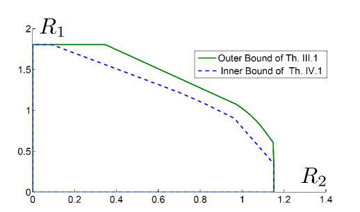
While we have analytically shown that the achievable rate region of Th. 5 achieves to within 3 bits/s/Hz the outer bounds in Th. 2, Fig. 4 shows, at least for certain channel parameters, that the gap from the less analytically tractable outer bound of Th. 1 is much less.

Figure 4: A comparison of the outer bounds of Th. 1 and Th. 2 and the inner bound of Th. 5 for the channel with $h_{11}=2h_{1c}=h_{2c}=h_{22}/5=1$.

VI Conclusion and Future Work

While the exact capacity of the GPC-CR is still unknown, we demonstrated inner and outer bounds which lie to within 3 bits/s/Hz from each other. This gap result was arrived at through insights gained from the capacity achieving schemes for the high-SNR linear deterministic approximation of the GPC-CR. We view this channel as a building block toward the more general IFC-CR in which interfering links between the two non-cognitive users are present. The PC-CR has allowed us to focus on the role of cognitive cooperation first, before incorporating interference created by the non-intended transmitter, which is the subject of ongoing work.

Appendix A Proof of Th.3

The capacity of the PC-CR in Fig. 1 is contained into the capacity of the transformed channel given in Fig. 3 where the input output relationship is described by:

$$\left[\begin{array}[]{l l l l l l l l l l}Y_{11}\\ Y_{1c}\end{array}\right] =\left[\begin{array}[]{l l l l l l l l l l}\;|h_{11}|X_{1}+Z_{11}\\ |h_{1c}|X_{c}+Z_{1c}\\ \end{array}\right]$$ (9e)

$$Y_{2} =|h_{22}|X_{2}+|h_{2c}|X_{c},$$ (9f)

where $Z_{11}\sim\mathcal{N}\left(0,\sigma_{11}^{2}\right)$, $\sigma_{11}^{2}\in[0,1]$, independent of $Z_{1c}\sim\mathcal{N}\left(0,1-\sigma_{11}^{2}\right)$, where the inputs are subject to $\mathbb{E}[|X_{i}|^{2}]\leq 1$, $i\in\{1,c,2\}$. Since $Y_{1}\sim Y_{11}+Y_{1c}$, the capacity of the transformed channel is no smaller than the capacity of the original channel. By Fano’s inequality:

$$N(R_{1}-\epsilon_{N})\leq I(Y_{11}^{N},Y_{1c}^{N};W_{1})$$

$$=I(Y_{11}^{N};W_{1})+I(Y_{1c}^{N};W_{1}|Y_{11}^{N})$$

$$\leq I(Y_{11}^{N};W_{1})+I(Y_{1c}^{N};W_{1}|Y_{11}^{N},W_{2})$$

$$=h(Y_{11}^{N})-h(Y_{11}^{N}|W_{1},X_{1}^{N})$$

$$+h(Y_{1c}^{N}|Y_{11}^{N},W_{2},X_{2}^{N})-h(Y_{1c}^{N}|Y_{11}^{N},W_{2},X_{2}^{N},W_{1},X_{1}^{N},X_{c}^{N})$$

$$\leq h(Y_{11}^{N})-h(Y_{11}^{N}|X_{1}^{N})$$

$$+h(Y_{1c}^{N}|X_{2}^{N})-h(Y_{1c}^{N}|X_{2}^{N},X_{c}^{N})$$ (10a)

$$=I(Y_{11}^{N};X_{1}^{N})+I(Y_{1c}^{N};X_{c}^{N}|X_{2}^{N})$$

$$\leq N\big{(}I(Y_{11};X_{1}|Q)+I(Y_{1c};X_{c}|X_{2},Q)\big{)},$$

where in (10a) we have used “conditioning reduces entropy” to drop $(Y_{11}^{N},W_{2})$ in $h(Y_{1c}^{N}|Y_{11}^{N},W_{2},X_{2}^{N})$ and the fact that $Y_{1c}^{N}$ is independent of everything else once conditioned on $X_{c}^{N}$.

For the sum-rate, by Fano’s inequality:

$$N(R_{1}+R_{2}-2\epsilon_{N})$$

$$\leq I(Y_{11}^{N},Y_{1c}^{N};W_{1})+I(Y_{2}^{N};W_{2})$$

$$\leq I(Y_{11}^{N},Y_{1c}^{N},Y_{2}^{N},W_{2};W_{1})+I(Y_{2}^{N};W_{2})$$

$$=h(Y_{2}^{N})-h(Y_{2}^{N}|W_{1},W_{2})$$

$$+I(Y_{11}^{N};W_{1}|Y_{2}^{N},W_{2})+I(Y_{1c}^{N};W_{1}|Y_{2}^{N},W_{2},Y_{11}^{N})$$

$$\leq I(Y_{2}^{N};X_{2}^{N},X_{c}^{N})$$

$$+I(Y_{11}^{N};X_{1}^{N})+I(Y_{1c}^{N};X_{c}^{N}|Y_{2}^{N},X_{2}^{N})$$ (11a)

$$=N\big{(}I(Y_{2};X_{2},X_{c}|Q)+I(Y_{11};X_{1}|Q)+I(Y_{1c};X_{c}|Y_{2},X_{2},Q)\big{)}$$

where (11a) follows from steps similar to those used to derive the $R_{1}$-bound. The outer bound is obtained as the union over all the distributions that factors $P_{Q,X_{1},X_{2},X_{c}}=P_{Q}P_{X_{1}|Q}P_{X_{2}|Q}P_{X_{c}|X_{1},X_{2},Q}$. Moreover, by the ”Gaussian maximizes entropy property” [7], we have that zero-mean complex Gaussian inputs maximize all the bounds in (5) and thus we let

$$\begin{pmatrix}X_{1}\\ X_{2}\\ X_{c}\\ \end{pmatrix}\sim\mathcal{N}\left(\bm{0},\begin{pmatrix}1&0&0\\ 0&1&\bar{\alpha}\\ 0&\bar{\alpha}^{*}&1\\ \end{pmatrix}\right).$$ (12)

Note that we can fix $\mathrm{Cov}(X_{1},X_{2})=0$ wlg since none of the rate bounds depends on the correlation of these two RVs. The expression in (5) is finally obtained by maximizing the sum rate bound of (11), with the inputs parametrization of (12), over the joint distribution of $P_{Y_{1},Y_{2}|X_{1},X_{2},X_{c}}$ for fixed marginals $P_{Y_{1}|X_{1},X_{2},X_{c}}$ and $P_{Y_{2},Y_{2}|X_{1},X_{2},X_{c}}$ as in [9].

Appendix B Proof of Th. 4

As in the proof of Th. 3, the capacity of the PC-CR in Fig. 1 is contained into the capacity of the transformed channel given in Fig. 3 where the input output relationship is described by:

$$\left[\begin{array}[]{l l l l l l l l l l}Y_{11}\\ Y_{1c}\end{array}\right] =\left[\begin{array}[]{l l l l l l l l l l}|h_{11}|X_{1}+Z_{11}\\ |h_{1c}|X_{c}+Z_{1c}\end{array}\right],$$ (13e)

$$\left[\begin{array}[]{l l l l l l l l l l}Y_{22}\\ Y_{2c}\end{array}\right] =\left[\begin{array}[]{l l l l l l l l l l}|h_{22}|X_{2}+Z_{22}\\ |h_{2c}|X_{c}+Z_{2c}\end{array}\right],$$ (13j)

for $Z_{11}\sim\mathcal{N}(0,\sigma_{11}^{2})$, $\sigma_{11}^{2}\in[0,1]$, independent of $Z_{1c}\sim\mathcal{N}(0,1-\sigma_{11}^{2})$, and $Z_{22}\sim\mathcal{N}(0,\sigma_{22}^{2})$, $\sigma_{22}^{2}\in[0,1]$ independent of $Z_{2c}\sim\mathcal{N}(0,1-\sigma_{22}^{2})$, and where the inputs are subject to $\mathbb{E}[|X_{i}|^{2}]\leq 1$, $i\in\{1,c,2\}$. Note the transformed channel in Fig. 3 consists of two point-to-point channels and a BC all in parallel. The original channel in Fig. 1 is a degraded version of the channel in Fig. 3 since $Y_{i}\sim Y_{ii}+Y_{ic}$, $i\in\{1,2\}$. As in the proof of Th. 3, we first show that independent coding across the parallel channels is optimal and then obtain the capacity region of the channel as the sum of the capacity of parallel channels. By Fano’s inequality:

$$N(R_{1}-\epsilon_{N})\leq I(Y_{11}^{N},Y_{1c}^{N};W_{1})$$

$$\leq I(Y_{1c}^{N};W_{1})+I(Y_{11}^{N};W_{1})$$ (14a)

$$\leq N\left(I(Y_{1c};X_{c}|U)+I(Y_{11};X_{1})\right)$$ (14b)

where (14a) follows from the same steps as (10), and (14b) from the rate bound for the degraded BC in [15], where the auxiliary random variable $U$ forms the Markov chain $U-X_{c}-Y_{1}-Y_{2}$ under the condition (7). Similarly we have that

$$N(R_{2}-\epsilon_{N})\leq I(Y_{22}^{N},Y_{2c}^{N};W_{1})$$

$$\leq I(Y_{2c}^{N};W_{1})+I(Y_{22}^{N};W_{1})$$ (15a)

$$\leq N\left(I(Y_{2c};U)+I(Y_{22};X_{1})\right)$$ (15b)

where (15a) follows from the same steps as (10) for user 2, and (15b) from the rate bound for the degraded BC in [15] for the same $U$ as in (14). The bounds of (14) and (15) do not depend on the joint distribution of $P_{X_{1},X_{2},X_{c}}$ but only on the marginal distribution of each RV. For this reason we can take $X_{c}\perp X_{1}$ and $X_{c}\perp X_{2}$ wlg while $X_{1}\perp X_{2}$ by definition. From this consideration and the “Gaussian maximizes entropy” property of [7], it follows that the optimal distribution of $X_{11}$ and $X_{22}$ is zero-mean complex Gaussian while from the “entropy power inequality” of [15] it follows that the optimal $U$ and $X_{c}$ must be proper complex Gaussian. The expression of (6) is obtained by noting that bounds are maximized when the power constraint is met with equality.

References

• [1] S. Rini, D. Tuninetti, and N. Devroye, “Outer Bounds for the Interference Channel with a Cognitive Relay,” Proc. IEEE Information Theory Workshop (ITW), Dublin, Ireland. Arxiv preprint arXiv:1004.4944, Sep. 2010.
• [2] O. Sahin and E. Erkip, “Achievable rates for the Gaussian interference relay channel,” in Proc. IEEE Global Telecommun. Conf. (GLOBECOM), 2007, pp. 1627–1631.
• [3] ——, “On achievable rates for interference relay channel with interference cancelation,” in Signals, Systems and Computers, 2007. ACSSC 2007. Conference Record of the Forty-First Asilomar Conference on.   IEEE, 2008, pp. 805–809.
• [4] J. Jiang, I. Maric, A. Goldsmith, and S. Cui, “Achievable rate regions for broadcast channels with cognitive radios,” Proc. of IEEE Information Theory Workshop (ITW), Taormina, Italy, pp. 500–504, Oct. 2009.
• [5] S. Sridharan, S. Vishwanath, S. Jafar, and S. Shamai, “On the capacity of cognitive relay assisted Gaussian interference channel,” in Proc. IEEE International Symposium on Information Theory (ISIT), Toronto, Canada, 2008, pp. 549–553.
• [6] S. Rini, D. Tuninetti, and N. Devroye, “New Inner and Outer bounds for the Interference Channel with a Cognitive Relay and capacity in Very Strong Interferenece,” Proc. IEEE International Symposium on Information Theory (ISIT), 2011 St. Petersburg, Russia, submitted to, 2010.
• [7] T. Cover, J. Thomas, and J. Wiley, Elements of Information Theory.   Wiley Online Library, 1991.
• [8] H. Sato, “An Outer Bound to the Capacity Region of Broadcast Channels (Corresp.),” IEEE Trans. Inf. Theory, vol. 24, no. 3, pp. 374–377, 1978.
• [9] S. Rini, D. Tuninetti, and N. Devroye, “Inner and outer bounds for the gaussian cognitive interference channel and new capacity results,” IEEE Trans. Inf. Theory, 2010, to be submitted.
• [10] ——, “New Inner and Outer Bounds for the Discrete Memoryless Cognitive Channel and Some Capacity Results,” IEEE Trans. Inf. Theory, 2010, accepted for publication, Arxiv preprint arXiv:1003.4328.
• [11] T. Han and K. Kobayashi, “A New Achievable Rate Region for the Interference Channel,” IEEE Trans. Inf. Theory, vol. 27, no. 1, pp. 49–60, Jan 1981.
• [12] J. Jiang, I. Maric, A. Goldsmith, and S. Cui, “Achievable Rate Regions for Broadcast Channels With Cognitive Relays,” Proc. IEEE Information Theory Workshop (ITW), Taormina, Italy, 2009.
• [13] S. Rini, D. Tuninetti, and N. Devroye, “Capacity of a Class of Gaussian Interference Channels with Cognitive Relays to within 3 bits/s/Hz,” IEEE Trans. Inf. Theory, 2011, to be submitted.
• [14] R. Etkin, D. Tse, and H. Wang, “Gaussian interference channel capacity to within one bit,” IEEE Trans. Inf. Theory, vol. 54, no. 12, pp. 5534–5562, 2008.
• [15] R. Gallager, “Capacity and Coding for Degraded Broadcast Channels,” Problems in the Transmission of Information, vol. 10, no. 3, pp. 3–14, 1974.