Math. Model. Nat. Phenom.

Vol. X, No. X, 2011, pp. 1-References

Viscous Shock Capturing in a Time-Explicit Discontinuous Galerkin Method

A. Klöckner^a, T. Warburton ^b and J. S. Hesthaven^c

^a Courant Institute of Mathematical Sciences, New York University, New York, NY 10012

^b Department of Computational and Applied Mathematics, Rice University, Houston, TX 77005

^c Division of Applied Mathematics, Brown University, Providence, RI 02912

Abstract. We present a novel, cell-local shock detector for use with discontinuous Galerkin (DG) methods. The output of this detector is a reliably scaled, element-wise smoothness estimate which is suited as a control input to a shock capture mechanism. Using an artificial viscosity in the latter role, we obtain a DG scheme for the numerical solution of nonlinear systems of conservation laws. Building on work by Persson and Peraire, we thoroughly justify the detector’s design and analyze its performance on a number of benchmark problems. We further explain the scaling and smoothing steps necessary to turn the output of the detector into a local, artificial viscosity. We close by providing an extensive array of numerical tests of the detector in use.

Key words: shock detection, Euler’s equations, discontinuous Galerkin, explicit time integration, shock capturing, artificial viscosity

AMS subject classification: 65N30, 65N35, 65N40, 35F61

1 Introduction

Discontinuous Galerkin methods [48, 43, 16, 31] are a high-order accurate, geometrically flexible, and robust means of approximating solutions of systems of hyperbolic conservation laws. For linear conservation laws, these schemes easily deliver highly accurate solutions without much effort. For nonlinear hyperbolic systems, the situation is more complicated. If the solution of the system remains smooth for the entire time under consideration, and if thereby the decay of modal coefficients is fast enough, the method may be used with little modification for a so-called “nodal approach”. Optionally, aliasing error in the computation of integrals for stiffness and mass matrices can be avoided by the introduction of quadrature schemes of sufficient order [31].

If however the solution does not stay smooth for long enough periods of time, the arising discontinuities pose a number of problems which have been the subject of intense study since the early days of scientific computation and numerical analysis. [e.g. 25, and references therein] Our goal is to seek out a method that is able to reliably detect the occurrence of Gibbs phenomena (which represent the main issue with the discontinuous solution) in the context of the discontinuous Galerkin method. In this paper, the subsequent mitigation of then phenomenon is then achieved through a simple artificial viscosity.

Many authors have proposed methods to capture shocks within a DG setting, by different methods. Flux limiting, which has been both successful and popular with Finite Volume practitioners, was combined with DG immediately in conjunction with the resurgence of interest in the method in the late 1980s. [13, 15, 16, 14, 10, 18, 56, 40, 39, 62]. A common theme to limiting is that the solution is modified in some way to retain desirable properties such as positivity and freedom from spurious oscillation, and in doing so, reaches various (often low) orders of accuracy.

Artificial viscosity methods, on the other hand, take the position that the only hope of resolving a discontinuity by a high-order approximation lies in smoothing it out. These methods date back to von Neumann and Richtmyer [57], were first used in the context of finite difference methods [41], and then spread into finite element literature (see, e.g., the study by John and Schmeyer [34] for a review) and were also applied to time-dependent discontinuous Galerkin methods very early on [5], and have since enjoyed continuing popularity [e.g. 11].

One obvious improvement on global artificial viscosities is a more selective application of smoothing, guided by a detector. There has been a recent resurgence of interest in such approaches [46, 4] in the context of DG. The methods discussed in this article aim to improve on these latter schemes, where we would like to emphasize that our detector is not intrinsically tied to guiding the application of an artificial viscosity. With appropriate rescaling, it might be suitable in a multitude of other scenarios requiring shock detection.

Other variants of artificial viscosity methods exist as well. The method of Spectrally Vanishing Viscosity [e.g. 55, 35] is similar in spirit, but tries to restrict its smoothing action to high-frequency solution components.

One final approach of dealing with discontinuities is that of adapting the mesh and adding resolution. It is generally thought that ‘shocks’, i.e. genuine discontinuities, do not exist in nature [61], and thereby, if only enough resolution were available, the problem of shock capturing would vanish by itself. While nature may obey this statement, mathematical models of it often do not (e.g. Burgers’ equation), and so one needs to “help a little”–for example by adding an artificial viscosity [e.g. 30]. Others contend that the wiggles are worth keeping simply as indicators of numerical trouble [27]. Further, while adaptivity certainly is a useful technique in capturing shocks [60, 24, 63], it too depends on a detector that reliably tells the method where refinement is necessary.

1.1 The Discontinuous Galerkin Method

Discontinuous Galerkin (DG) methods [48, 43, 16, 31] are a combination of ideas from Finite-Volume and Spectral Element methods. We consider DG methods for the approximate solution of a hyperbolic system of conservation laws

$$u_{t}+\nabla\cdot F(u)=0$$ (1.1)

on a domain $\Omega=\biguplus_{k=1}^{K}\mathsf{D}_{k}\subset\mathbb{R}^{d}$ consisting of disjoint, face-conforming tetrahedra $\mathsf{D}_{k}$ with boundary conditions

$$u|_{\Gamma_{i}}(x,t)=g_{i}(u(x,t),x,t),\hskip 20.00003pti=1,\ldots,b,$$

at inflow boundaries $\biguplus\Gamma_{i}\subseteq\partial\Omega$. We find a weak form of (1.1) on each element $\mathsf{D}_{k}$:

$$0=\int_{\mathsf{D}_{k}}u_{t}\varphi+[\nabla\cdot F(u)]\varphi\,\mathrm{d}x=\int_{\mathsf{D}_{k}}u_{t}\varphi-F(u)\cdot\nabla\varphi\,\mathrm{d}x+\int_{\partial\mathsf{D}_{k}}(\hat{n}\cdot F)^{\ast}\varphi\,\mathrm{d}S_{x},$$

where $\varphi$ is a test function, and $(\hat{n}\cdot F)^{\ast}$ is a suitably chosen numerical flux in the unit normal direction $\hat{n}$. Following [31], we may find a so-called ‘strong’-DG form of this system as

$$0=\int_{\mathsf{D}_{k}}u_{t}\varphi+[\nabla\cdot F(u)]\varphi\,\mathrm{d}x-\int_{\partial\mathsf{D}_{k}}[\hat{n}\cdot F-(\hat{n}\cdot F)^{\ast}]\varphi\,\mathrm{d}S_{x}.$$ (1.2)

by integrating by parts once more. We seek to find a numerical vector solution $u^{k}:=u_{N}|_{\mathsf{D}_{k}}$ from the space $P_{N}^{n}(\mathsf{D}_{k})$ of local polynomials of maximum total degree $N$ on each element, where $n$ is the number of equations in the hyperbolic system (1.1). We choose the scalar test function $\varphi\in P_{N}(\mathsf{D}_{k})$ from the same space and represent both by expansion in a basis of $N_{p}:=\operatorname{dim}P_{N}(\mathsf{D}_{k})$ Lagrange polynomials $l_{i}$ with respect to a set of interpolation nodes [58]. We define the mass, stiffness, differentiation, and face mass matrices

$$M_{ij}^{k} :=\int_{\mathsf{D}_{k}}l_{i}l_{j}\,\mathrm{d}x, S_{ij}^{k,\partial\nu} :=\int_{\mathsf{D}_{k}}l_{i}\partial_{x_{\nu}}l_{j}\,\mathrm{d}x,$$ (1.3a)

$$D^{k,\partial\nu} :=(M^{k})^{-1}S^{k,\partial\nu}, M_{ij}^{k,A} :=\int_{A\subset\partial\mathsf{D}_{k}}l_{i}l_{j}\,\mathrm{d}S_{x}.$$ (1.3b)

Using these matrices, we rewrite (1.2) as

$$0 =M^{k}\partial_{t}u^{k}+\sum_{\nu}S^{k,\partial_{\nu}}[F(u^{k})]-\sum_{F\subset\partial\mathsf{D}_{k}}M^{k,A}[\hat{n}\cdot F-(\hat{n}\cdot F)^{\ast}],$$

$$\partial_{t}u^{k} =-\sum_{\nu}D^{k,\partial_{\nu}}[F(u^{k})]+L^{k}[\hat{n}\cdot F-(\hat{n}\cdot F)^{\ast}]|_{A\subset\partial\mathsf{D}_{k}}.$$ (1.4)

The matrix $L^{k}$ used in (1.4) deserves a little more explanation. It acts on vectors of the shape $[u^{k}|_{A_{1}},\dots,u^{k}|_{A_{4}}]^{T}$, where $u^{k}|_{A_{i}}$ is the vector of facial degrees of freedom on face $i$. For these vectors, $L^{k}$ combines the effect of applying each face’s mass matrix, embedding the resulting facial values back into a volume vector, and applying the inverse volume mass matrix. Since it “lifts” facial contributions to volume contributions, it is called the lifting matrix. Its construction is shown in Figure 1.

Figure 1: Construction of the Lifting Matrix $L^{k}$.

It deserves explicit mention at this point that the left multiplication by the inverse of the mass matrix that yields the explicit semidiscrete scheme (1.4) is an element-wise operation and therefore feasible without global communication. This strongly distinguishes DG from other finite element methods. It enables the use of explicit (e.g., Runge-Kutta) time stepping and greatly simplifies parallel implementation efforts.

2 Basic Design Considerations

This article describes a method for detecting (and also capturing) shocks in the context of DG methods. One particular motivation for us was our recent work on the efficient mapping of DG onto massively parallel throughput-oriented computer architectures [36], where we demonstrated a method to quickly compute the vector $A(x)$ for a linear discontinuous Galerkin operator $A$ and a state vector $x$ using graphics hardware (i.e. Graphics Processing Units or “GPUs”). The present article describes one stepping stone on the way to generalizing the applicability of GPU-DG to nonlinear problems.

In briefly explaining the unique environment present on GPUs, we seek to inform the reader on the considerations that guided our approach. On wide-SIMD, parallel architectures such as the GPUs of [36], memory is at a premium and scattered memory access is particularly expensive. As a consequence, we argue that matrix-free methods such as the one of [36], if they can be implemented efficiently, will always hold a significant performance advantage over approaches that have to build, keep in memory, and constantly access a pre-built sparse matrix for $A$, because such a computation is necessarily bound by the speed at which matrix entries can be streamed into the core, where they are then used exactly once and discarded [7]. A matrix-free approach has far more freedom to exploit local structure and re-use data. We will therefore focus our investigation on matrix-free methods.

This choice has important ramifications. One consequence of it affects the trade-off by which one chooses between implicit and explicit time stepping. Consider the case of implicit time integrators, in which one must constantly solve large linear systems of equations. Direct, factoring solvers for sparse matrices are as yet unavailable on massively parallel hardware, and even if they were, they would doubly suffer from the issues that sparse matrices encounter. One therefore naturally looks towards iterative methods for solving large sparse systems. For the complicated linearized systems arising from the nonlinear hyperbolic conservation laws we are targeting in this article, these methods generally need help in the form of a preconditioner in order to be efficient. This is the next implication of the choice of matrix-free methods: One automatically chooses to not use the substantial body of literature showing how a preconditioner may be built from a known sparse matrix. Instead, one needs to invest further work designing and testing preconditioners (using e.g. multi-grid or domain-decomposition methods), and, in addition to the design time spent, these preconditioners may carry significant additional computational expense, typically through their communication needs. In addition, Krylov methods (which are frequently used to solved the arising large, sparse linear systems) in particular involve global reductions (in the form of inner products) which are known to not achieve peak performance on graphics processors [29]. Worse, the nonlinear PDEs we are targeting in this paper require a nonlinear system of equations to be solved (likely by Newton iteration, which in turn requires Jacobians to be evaluated).

This collection of drawbacks and uncertainties in the application of implicit time integration on massively parallel hardware makes it seem opportune to examine the use of explicit time steppers, which were already used with good success in [36]. We aim to find out if the single big disadvantage of explicit methods, namely their small time step restriction, can be offset by the judicious choice of methods combined with the advantages conferred by the hardware.

Since the scheme we are aiming to design involves the use of artificial viscosity, the scaling of the explicit time step is typically given by

$$\Delta t\sim\frac{1}{\displaystyle\lambda_{\text{max}}\frac{N^{2}}{h}+\|\nu\|_{L^{\infty}}\frac{N^{4}}{h^{2}}},$$ (2.1)

where $\lambda_{\text{max}}$ is the largest characteristic velocity and $\nu$ is the magnitude of the viscosity, $h$ is the local mesh size and $N$ is the approximation’s polynomial degree [31]. Within (2.1), the numerical diffusion time scale $N^{4}\|\nu\|_{L^{\infty}}/h^{2}$ can be rather damaging, as it contains discretization-dependent factors at high exponents.

Luckily, (2.1) does not tell the entire story. For example, we expect the occurrences of high viscosity $\nu$ to be localized in both space and time. Localization in space could conceivably be dealt with using local time stepping, but this is beyond the scope of this article. Localization in time on the other hand is easily dealt with by the use of time-adaptivity [e.g. 19]. Adaptivity in time is particularly important for explicit time stepping of artificial-viscosity-enhanced PDE solvers.

One further aspect of the time discretization should be considered: Much of the effort in this research is targeted at mitigating the effect of oscillations in the spatial discretization of a conservation law that trace their roots back to the polynomial expansions used for them. Time discretizations, however, are equally based on polynomials, and many varieties of so-called Strong Stability Preserving (SSP) time integrators have been devised to mitigate oscillations originating in temporal expansions [50]. Even embedded pairs of SSP Runge-Kutta methods are available [26]. Based on initial experiments, it appears that in the setting of this work, spatially-generated oscillations by far dominate their temporal cousins at the time step sizes encountered. Thus varying the time integration method does not have an appreciable effect on the reported results.

In summary, the emergence of massively parallel hardware along with the use of purposefully chosen, adaptive time discretizations may help explicit methods be competitive with implicit methods for the integration of large-scale nonlinear systems, a few of which we will introduce next.

3 Applications and Equations

3.1 Advection Equation

At the very simple end of the spectrum of hyperbolic conservation laws, the advection equation $\partial_{t}u+v\cdot\nabla_{x}u=0$ transports its initial condition along its one characteristic, described by the velocity vector $v$. We will apply artificial viscosity to this PDE as

$$\partial_{t}u+v\cdot\nabla_{x}u=\nabla_{x}\cdot(\nu\nabla_{x}u).$$

Here, and in all further equations, it is important to write the viscosity in “conservation” form $\nabla_{x}\cdot(\nu\nabla_{x}u)$. The desired consequence of this is that the resulting DG method will be conservative [1].

In DG discretizations of this equation, we use a conventional upwind flux in a strong-form DG formulation. The diffusion term $\nabla_{x}\cdot(\nu\nabla_{x}u)$ is discretized by a first-order (“dual”) interior penalty method [1], with the gradient being computed in strong form, and the divergence computed in weak form. The diffusive fluxes are given by

$$u_{N}^{\ast}:=\{u_{N}\},\qquad\sigma_{N}^{\ast}:=\{\nu\nabla_{x,h}u_{N}\}-\frac{N^{2}}{h}\nu\left\llbracket u_{h}\right\rrbracket,$$

where $\sigma_{N}$ is the discretization of $\nu\nabla_{x}u$.

3.2 Second-Order Wave Equation

The wave equation $\partial t^{2}u+c^{2}\triangle u=0$ is valuable for testing artificial viscosity methods because it is the simplest system where the effects of two coupled characteristics may be observed. We rewrite this PDE as a first-order system of conservation laws and apply artificial viscosity to this system to obtain

$$\partial_{t}u+c\nabla_{x}\cdot v =\nabla_{x}\cdot(\nu\nabla_{x}u),$$ (3.1a)

$$\partial_{t}v+c\nabla_{x}u =\nabla_{x}\cdot(\nu\nabla_{x}v),$$ (3.1b)

where we have again been careful to use the conservative form of the diffusive term. The vector diffusion term $\nabla_{x}\cdot(\nu\nabla_{x}v)$ is to be read as the diffusion $\nu$ being applied to each component separately. The discontinuity sensor to be described below operates on the scalar component $u$. In DG discretizations of this equation, we again use a conventional upwind flux in a strong-form DG formulation. The diffusion terms are discretized in analogy to the preceding section.

3.3 Euler’s Equations of Gas Dynamics

Lastly, the system of conservation laws that justifies the effort spent on this study, Euler’s equations of gas dynamics, broadly applies to compressible, inviscid flow problems. As in Section 3.2, we are again choosing to use a single artificial viscosity $\nu$ that applies to all components, such that we get the viscosity-endowed system

$$\partial_{t}\rho+\nabla_{x}\cdot(\rho\mathbf{u}) =\nabla_{x}\cdot(\nu\nabla_{x}\rho),$$ (3.2a)

$$\partial_{t}(\rho\mathbf{u})+\nabla_{x}\cdot(\mathbf{u}\otimes(\rho\mathbf{u}))+\nabla_{x}p =\nabla_{x}\cdot(\nu\nabla_{x}(\rho\mathbf{u})),$$ (3.2b)

$$\partial_{t}E+\nabla_{x}\cdot(\mathbf{u}(E+p)) =\nabla_{x}\cdot(\nu\nabla_{x}E).$$ (3.2c)

The discontinuity sensor to be described below operates on the component $\rho$. In contrast to Persson and Peraire [46], we find that a Navier-Stokes-like physical viscosity provides insufficient control of oscillations in $\rho$.

In DG discretizations of this system, a local Lax-Friedrichs (or Rusanov) flux

$$\hat{n}\cdot F_{N}^{\ast}:=\hat{n}\cdot\frac{F(u^{+})+F(u^{-})}{2}-\frac{\lambda_{\text{max}}}{2}(u^{+}-u^{-}),$$

in weak-form DG is commonly used. The diffusion term is discretized as in Section 3.2. As above, a quadrature exact to degree $3N$ is used to integrate the nonlinearity.

4 A Smoothness-Estimating Detector

Detectors for the selective application of artificial viscosity have been built in a large variety of ways. The most popular, perhaps, is sensing on the $L^{2}$ norm of the residual of the variational form [5, 33]. Hartmann [30] employs a similar indicator that includes sensing of the primary orientation of the discontinuity and performs anisotropic mesh refinement based on this data.

Other detectors in the literature employ information gathered not on the whole volume of the domain, but only on element faces [6]. Specializing further, some methods use the magnitude of the facial inter-element jumps as an indicator of how well-resolved the solution is and to what degree it has converged [4, 23]. A further approach to shock detection repurposes entropy pairs, objects from the solution theory for scalar conservation laws, for the purposes of shock detection [28].

Our approach most directly traces its lineage to work by Persson and Peraire [46], which addresses one crucial shortcoming in much of the above work: scaling. Many of the quantities discussed clearly relate directly to how well-resolved (and smooth) the approximate solution of the system is. It is however rarely clear how large a value of the quantity in question indicates that a problem exists, and a variety of ad-hoc scaling choices are proposed, often by the maximum of the quantity found across the domain, or by the element-local norm, but without assigning an explicit meaning to the scaled quantity.

The method by Persson and Peraire [46] also performs scaling by the element-local $L^{2}$ norm $\|q_{N}\|_{L^{2}(\mathsf{D}_{k})}$ of the discretized value of the quantiy $q_{N}$ to be sensed on. On each element $\mathsf{D}_{k}$, it obtains a value

$$S_{k}:=\frac{(q_{N},\phi_{N_{p}-1})^{2}_{L^{2}(\mathsf{D}_{k})}}{\|q_{N}\|^{2}_{L^{2}(\mathsf{D}_{k})}},$$ (4.1)

where $\{\phi_{n}\}_{n=0}^{N_{p}-1}$ is an orthonormal basis for the expansion space [see e.g. 20, 37] numbered from 0. Simply put, $S_{k}$ reflects the (squared) fraction of $q_{N}$’s mass contained in the highest mode of the expansion, relative to all mass present on the element. Persson and Peraire [46] then invoke an analogy to Fourier expansions, where a continuous function (roughly) can be recognized by having Fourier expansions in which the $n$th mode’s magnitude scales at most as $1/n^{2}$. In doing so, they have conveniently solved the issue of scaling–it is now understood what $S_{k}$ measures and what value it is supposed to take on for which degree of smoothness. Based on this analogy, they argue that $S_{k}$ should have a magnitude of $1/N^{4}$ for $q_{N}$ to be continuous, or, alternatively, that smoothing by artificial viscosity should activate if $S_{n}>1/N^{4}$.

They achieve this activation through a sequence of mapping steps. First, they take the logarithm

$$s_{k}:=\log_{10}S_{k}$$

to obtain a quantity that scales linearly with the decay exponent, which they put in relation to a quantity $s_{0}$ that they claim should scale as $1/N^{4}$. We believe this is a typographical error in their paper, because for proper comparability, $s_{0}$ should scale with the logarithm of $1/N^{4}$. Through the application of a mapping, they obtain the final per-element viscosity

$$\nu_{k}(s_{k})=\nu_{0}\begin{cases}0&s_{k}<s_{0}-\kappa,\\ \frac{1}{2}\left(1+\sin\frac{\pi(s_{k}-s_{0})}{2\kappa}\right)&s_{0}-\kappa\leq s_{k}\leq s_{0}+\kappa,\\ 1&s_{0}+\kappa<s_{k},\end{cases}$$ (4.2)

where $\nu_{0}$ is the maximum viscosity, which Persson and Peraire [46] suggest to scale with $h/N$ and $\kappa$ is the width of the activation “ramp”.

The focus of the remainder of this article is to identify a number of issues and make a number of improvements to this method of finding an artificial viscosity.

4.1 Estimating Solution Smoothness

Before we begin our discussion of the refinements to the method, let us set the stage by discussing the type of numerical method at which the to-be-designed detector is aimed. As was already discussed, for methods of low approximation order (and polynomial degrees $N\lessapprox 2$), the flux limiting literature provides plenty of alternatives for shock capturing, and therefore will not be the main target area for our work. Since our method, like the work of Persson and Peraire [46], will try to extract smoothness information from the modal expansion of the solution, it is our hope that the expansion at these degrees already contains enough smoothness information to be viable as a basis for an artificial viscosity. Lastly, at degrees $N\gtrapprox 5$, there is guaranteed to be sufficient smoothness information, though the time step restriction (2.1) may make these approximations somewhat impractical.

We begin our deconstruction and rebuild of the Peraire-Persson estimator by examining the assumption that, like for Fourier series, smoothness can be estimated by modal decay. In Fourier series, this can be justified by viewing what happens if a derivative of an expanded function is taken (and hence smoothness is reduced)–the $n$th coefficient’s magnitude gets multiplied by $n$. This results in the identity

$$\left\|\frac{d}{dx}e^{inx}\right\|_{L^{p}((-\pi,\pi))}=n\left\|e^{inx}\right\|_{L^{p}((-\pi,\pi))}\qquad\text{for $p\in[1,\infty]$}.$$ (4.3)

A polynomial analog for (4.3) is provided by Bernstein’s inequality [59, 9]

$$\left|\frac{d}{dx}P(x)\right|\leq\frac{n}{\sqrt{1-x^{2}}}\|P(x)\|_{L^{\infty}([-1,1])}\qquad\text{for $P\in P^{n}([-1,1])$, $x\in[-1,1]$}.$$ (4.4)

While it conveniently exhibits the same scaling as its Fourier counterpart, unfortunately, this estimate breaks down near the domain boundaries. Markov’s inequality

$$\left\|\frac{d}{dx}P(x)\right\|_{L^{\infty}([-1,1])}\leq n^{2}\left\|P(x)\right\|_{L^{\infty}([-1,1])}\qquad\text{for $P\in P^{n}([-1,1])$}.$$ (4.5)

extends the estimate out to the domain boundary, at the expense of a larger scaling. Further, it may be argued that if one wants to transfer the knowledge gained from (4.5) to a modal setting, $L^{\infty}$ is the wrong norm, and one should consider the $L^{2}$ norm instead to be able to benefit from Parseval’s identity. Fortunately, an $L^{2}$ analog of (4.5) is available [59, and references therein]

$$\left\|\frac{d}{dx}P(x)\right\|_{L^{2}([-1,1])}\leq\sqrt{3}n^{2}\left\|P(x)\right\|_{L^{2}([-1,1])}\qquad\text{for $P\in P^{n}([-1,1])$},$$ (4.6)

known as an inverse inequality. Taking into account (4.4) and (4.6), the polynomial analogy to the Fourier case is therefore expected to carry over well for non-smoothness occurring on the interior of each finite element, whereas for non-smoothness at the domain boundary, the smoothness measure will likely differ.

Having examined the viability of modal decay as an estimator for smoothness, we seek to make the notion of modal decay more precise than (4.1). We presume that, for the modal coefficients $\{\hat{q}_{n}\}_{n=0}^{N_{p}-1}$ of a member $q_{N}$ of the $L^{2}$-orthonormal approximation space spanned by $\{\phi_{n}\}_{n=0}^{N_{p}-1}$, modal decay is approximately representable as

$$|\hat{q}_{n}|\sim cn^{-s}.$$ (4.7)

Taking the logarithm of the relationship (4.7) yields

$$\log|\hat{q}_{n}|\sim\log(c)-s\log(n),$$

an affine relationship whose coefficients $s$ and $log(c)$ may be found through least-squares fitting, satisfying

$$\sum_{n=1}^{N_{p}-1}\left|\log|\hat{q}_{n}|-(\log(c)-s\log(n))\right|^{2}\rightarrow\min!$$ (4.8)

Observe that the decay rate of (4.7) has rather little to do with the presumed magnitude of the remainder term of an expansion, on which most a-priori error estimates for finite element solutions are based–these start with an assumption of sufficient smoothness. There is a connection, however. Mavriplis [45], in the context of mesh adaptation, has used a similar least-squares fit to the modal decay, defining a continuous function $\hat{q}(n)$ through the found fit. She then proceeds to estimate the remainder term of the expansion as

$$\|q-q_{N}\|_{L^{2}(\mathsf{D}^{k})}^{2}\approx\left(\frac{\hat{q}_{N}^{2}}{\frac{2N+1}{2}}+\int_{N+1}^{\infty}\frac{\hat{q}(n)^{2}}{\frac{2n+1}{2}}\,\mathrm{d}n\right).$$

In a similar vein, Houston and Süli in [32] use an $l^{2}$ fit like (4.8) as a criterion for $hp$-adaptive refinement. They obtain the approach from a discussion of results in approximation theory [17].

Figure 2: Modal portrait for an approximant of a (discontinuous) Heaviside jump function. Subfigure (a) shows the nodal data and its unique polynomial interpolant. Subfigure (b) shows the modal coefficients of a Legendre expansion of the function in (a), the processing of these coefficients, and the unprocessed and postprocessed smoothness estimates.

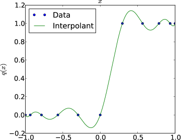
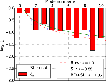
The least-squares procedure (4.8) yields an estimate $s$ of the decay exponent. If the analogy with Fourier modal decay holds up, one would then expect $s\approx 1$ for a discontinuous $q$, $s\approx 2$ for $q\in C^{0}\setminus C^{1}$, $s\approx 3$ for $q\in C^{1}\setminus C^{2}$, and so forth. Figure 2 shows a first attempt at determining whether this is really the case by examining an interpolant of a Heaviside jump function $H$ as shown in Figure 2. Figure 2 shows the magnitudes of the first ten modal coefficients along with the fitted curve (the dashed red line). The obtained decay exponent $s$, shown in the legend next to the dashed red line, matches the expectation well, giving a value of exactly 1.

Figure 3: Modal portrait for an approximant of a $C^{0}$ non-differentiable “kink” function.

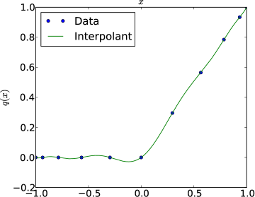
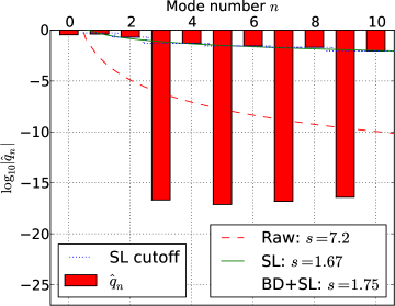
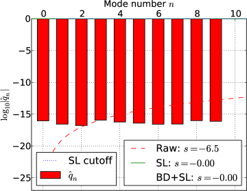
Continuing this line of experimentation, we would like to move on to an interpolant of a “kink” function $q(x):=xH(x)$. The same observations as for the Heaviside function are shown in Figure 3. Unfortunately, the figure reveals a rather powerful shortcoming of the modal fit method as developed so far. An odd-even effect draws the coefficients for the odd modes of number three and greater to zero, leading to machine zeros ($\approx 10^{-15}$) in those approximate coefficient numbers. These “fully converged” coefficients fool the estimator into an anomalous estimate of far more smoothness than is actually present, leading to an estimated decay exponent of about seven–far too high.

It is unfortunate that the fit can be misled that easily, but a close look at Figure 3 will have already revealed to the attentive reader that this is an easily recoverable issue. Realize that the fit tries to model modal decay, i.e. the shrinking of modal coefficient magnitudes $|\hat{q}_{n}|$ as $n$ increases. The model (4.7) that is fitted to the decay only generates monotone modal decays. Figure 3 is characterized by a strongly non-monotone mode profile, and this is precisely what is misleading the estimator. Consider this: Given a mode $n$ with a small coefficient $|\hat{q}_{n}|$, if there exists another coefficient with $m>n$ and $|\hat{q}_{m}|\gg|\hat{q}_{n}|$, then the small coefficient $|\hat{q}_{n}|$ was likely spurious, just like the near-zero coefficients in Figure 3 were spurious. These spurious coefficients should hence be eliminated from the fit, and this is what a new procedure, termed skyline pessimization, achieves. From the modal coefficient magnitudes $\{|\hat{q}_{n}|\}_{n=0}^{N_{p}-1}$, it generates a new set of modal coefficients by

$$\bar{q}_{n}:=\max_{i\in\{\min(n,N_{p}-2),\dots,N_{p}-1\}}|\hat{q}_{i}|\qquad\text{for $n\in\{1,2,\dots,N_{p}-1\}$}.$$ (4.9)

The effect of the procedure is that each modal coefficient is raised up to the largest higher-numbered modal coefficient, eliminating non-monotone decay. Since odd-even effects in modal portraits (such as the one of Figure 3 are a common phenomenon, there is a slight modification in (4.9) accounting for the last mode, which is forced to also be larger than the second-to-last mode. This would become an issue if, for example, only the first nine modes of Figure 3 were used, in which case the smallness of the last coefficient would again cause an artificially high smoothness exponent. Once skyline pessimization has been performed, decay estimation (4.8) is applied to them in the same fashion as above, yielding a corrected decay estimate.

The effect of skyline pessimization is shown in the modal portrait of Figure 3 as a zig-zagged blue line that appears to “truncate” the bars representing modal coefficients at the level of the largest higher-numbered coefficient. Further, the fitted decay curve is shown in green, along with the resulting estimated decay exponent, labeled as “SL”. With skyline pessimization in place, the estimated smoothness exponent for the “kink” example becomes 1.67–reasonably close to the expected value of 2.

Figure 4: Modal portrait for a function consisting of only the highest representable Legendre mode $\phi_{N_{p}-1}$ in an expansion of length 10.

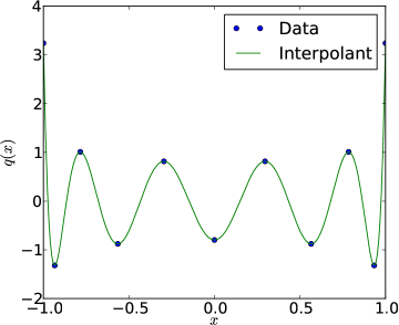
The next-smoothest test of the estimator we consider is a truncated polynomial $q(x):=x^{2}H(x)$. Obviously, $q\in C^{1}\setminus C^{2}$. As in the “kink” case, the modal decay exhibits a pronounced odd-even discrepancy (not shown), that leads to spuriously high “raw” smoothness exponent estimate of about 13. After skyline pessimization, the estimate assumes nearly exactly the expected value, three. The three artificial tests conducted so far confirm the premise on which the estimator is built, namely that the smoothness of a function represented by a Legendre expansion can be accurately estimated solely by examining its coefficients.

By presenting a number of further tests, we hope to clarify the behavior of the estimator as designed so far. A particularly interesting case is shown in Figure 4, which shows the estimator applied to the highest mode present in the Legendre expansions of length 10 which we have been considering. In a sense, this is the most oscillatory, and thereby the least smooth, function that the expansion can express. After skyline pessimization, this function is assigned a smoothness exponent of zero–which in a Fourier setting would correspond to white noise.

The next two tests are concerned with very smooth functions ($\cos(3+\sin(1.3x))$ and $\sin(\pi x)$) and confirm that the estimator recognizes them as such. While the smoothness values (both around four) assigned to them are not as meaningful as the results in the low-smoothness examples, this is not necessarily a problem. As long as the estimator can sharply pick up non-smoothness on a reliable scale (and keep the smooth examples clear of this area), it is performing satisfactorily for its purpose.

The second-to-last test highlights a behavior of the detector that could be considered a failure mode. Consider a constant function perturbed by white noise of a much smaller scale. As discussed above, the detector ignores the constant and only ‘sees’ white noise, yielding a smoothness value of about zero. This behavior is undesirable, as the detected smoothness value may depend on the presence or absence of mere floating point noise. One root of this problem is the removal of constant-mode information from the estimation process, causing the estimator to not have a “sense of scale”, i.e. keeping it from noticing that the noise is “small” compared to the remainder of the solution. In the following, we present one way to re-add this “sense of scale” by distributing energy according to a “perfect modal decay”

$$|\hat{b}_{n}|\sim\frac{1}{\sqrt{\sum_{i=1}^{N_{p}-1}\frac{1}{n^{2N}}}}\frac{1}{n^{N}}$$ (4.10)

for $N$ the polynomial degree of the method, where the normalizing factor ensures that

$$\sum_{n=1}^{N_{p}-1}|\hat{b}_{n}|^{2}=1.$$

The idea is to consider the coefficients

$$|\tilde{q}_{n}|^{2}:=|\hat{q}_{n}|^{2}+\|q_{N}\|^{2}_{L^{2}(\mathsf{D}_{k})}|\hat{b}_{n}|^{2}\qquad\text{for $n\in\{1,\dots,N_{p}-1\}$}$$ (4.11)

as input to skyline pessimization instead of the “raw” coefficients $|\hat{q}_{n}|^{2}$. This amounts to adding baseline modal decay scaled by the element-wise norm that will ‘drown out’ the floating point noise.

For the sake of exposition, baseline decay was not introduced initially. The reader may convince himself that its introduction does not unduly modify experimental results so far by examining the estimated decay exponents given as “BD+SL” in the past graphs and comparing to the pure-skyline values given as “SL”.

Figure 5: Modal portrait for an approximant of a (discontinuous) jump function, offset from the center of the element.

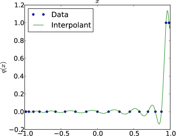
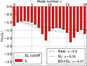
This completes the discussion of the design of the detector. Now might also be a good time to point out a known shortcoming in its design that was already anticipated in the motivating discussion. The issue relates to the discussion of mode scaling with decreasing smoothness initiated earlier in this section. Consider Figure 5, which shows decay estimation data for the same Heaviside jump function as Figure 2, but shifted to the element’s edge. The data in the figure confirms the earlier conjecture that a function with a sharply localized non-smoothness might result in modal decay exponents that differ by up to a factor of two, depending on where the non-smoothness is located inside the element–the measured smoothness exponent for the shifted Heaviside function is only 0.57, compared to 1.05 after all corrections above. Additional confirmation comes from the fact that the final smoothness estimates for boundary-shifted versions of the kink and the $C^{1}$ spline are $s=1.19$ and $s=2.24$ respectively (not shown). This relates in striking ways to the scaling of the DG CFL condition (2.1), and like in its case, an entirely practical remedy for this issue is not yet known.

Based on the shown examples, it should be clear that even the unassisted decay fit is a more robust smoothness estimator than the single-mode indicator (4.1), if only for the simple reason that it considers a much broader set of modal data. But we have shown that even this fairly robust indicator can give poor results in surprisingly common cases. We feel that this strongly supports the statement that the decay fit indicator with skyline pessimization and added baseline decay represents a more practical–if slightly more expensive–way of obtaining smoothness information on a numerical solution.

5 From Smoothness to Viscosity

5.1 Scaling the Viscosity

This section assumes that the output of the indicator is an estimated decay exponent $s$, approximating the decay of the solution’s modal coefficients as $|\hat{u}_{n}|\sim n^{-s}$. We are seeking to design an activation function $\nu(s)$ whose value is the viscosity coefficient.

For the interpretation of the decay exponent $s$, recall the targeted scaling of the smoothness exponent $s$, where (roughly) $s=1$ would indicate a discontinuous solution, $s=2$ would indicate a $C^{0}$ solution, $s=3$ a $C^{1}$ solution, and so forth. Among the chief nuisances of polynomial approximations that this work seeks to remedy is the Gibbs phenomenon, which occurs for discontinuous solutions ($s=1$). We therefore expect to have $\nu(1)=\nu_{0}$, where $\nu_{0}$ is the maximum value of $\nu$ and dictates its scaling. Merely continuous functions still pose somewhat of a problem for polynomial approximation, so we arbitrarily fix $\nu(2)=\nu_{0}/2$, and finally we fix $\nu(3)=0$, as we prefer that $C^{1}$ solutions should not be modified by viscosity.

Given the activation map $\nu_{k}(s_{k})$ of (4.2) with the fixed values $s_{0}=2$, the map $\nu(s):=1-\nu_{k}(s_{k})$ with the fixed values $s_{0}=2$ and $\kappa=1$ provides such a ramp. (Observe that in (4.2), decreasing values indicate more smoothness, while this work uses the opposite convention.) Because of the close attention paid to precise scaling of the smoothness $s$, we were able to fix values for the ramp location and width parameters $\kappa$ and $s_{0}$.

To find an appropriate value $\nu_{0}$, the behavior of the diffusion term needs to be investigated. To this end, we examine the fundamental solution of the diffusion equation $u_{t}=\nu\triangle u$, the heat kernel. Adopting the probabilistic standard deviation $\sigma$ as a measure of width, the heat kernel after time $t$ has a width of $\sigma=\sqrt{2\nu t}$. Considering some unit $t$ of time, the conservation law will propagate information to a distance of $\lambda$, where $\lambda$ is some local characteristic velocity. Observe that viscosity propagates the bulk of its mass at a non-linear square-root pace, while the conservation law observes a linear speed. One therefore needs to pick a reference time scale $t$ as well as a reference distance at which the two propagation distances are to coincide.

Choosing $\sigma=h/N$ after $t=(N/2)\Delta t$, and approximating $\Delta t\approx h/(\lambda N^{2})$, one obtains

$$\nu_{0}=\frac{\sigma^{2}}{2t}=\lambda\frac{h}{N}.$$ (5.1)

This reproduces the value of Barter and Darmofal [4] and simultaneously provides some more detailed insight into its meaning. We would like to note that $\sigma=h/N$ is probably too ambitious a goal, as this would only smooth discontinuities to a with of about the distance between two nodal points–likely too little as Figure 2 shows. A choice of $\sigma=3h/N$ has proven to be more realistic.

For a system of conservation laws, there remains the question of which characteristic velocity should be chosen for $\lambda$. This choice has important implications as, e.g. in the Euler system, contact discontinuities propagate with stream velocity, whereas shocks propagate at sonic speeds. In a one-dimensional setting, Rieper [49] convincingly argues that the best course of action is to perform smoothing in characteristic variables, so that each wave receives the amount of smoothing specified by the scheme, e.g. as given in (5.1). Observe that doing may work well in one-dimension and for low-order multi-D finite volume schemes, but it is less clear how it might be applied in a genuinely multidimensional situation. A simple and functional strategy is to choose $\lambda$ to be the maximum characteristic velocity $\lambda_{\text{max}}$. The simplicity of this strategy comes at a price, however: returning to the example of the Euler equations, contact discontinuities have their $\nu_{0}$ set higher than would be necessary from this analysis, and our numerical experiments will reflect this.

Thus the $\lambda_{\max}$-based scaling is not perfect. It works, in the sense that all test examples run successfully using it, but some can benefit from an additional ‘fudge factor’. For example, while problems involving Burgers’ equation (not shown) work well with an unmodified scaling in a ’picture norm’ sense (little oscillation, least smoothing), most subsonic Euler problems benefit from the application of an additional factor of $1/2$. This is not entirely unexpected, given the above discussion.

5.2 Smoothing the Viscosity

The artificial viscosity $\nu(x)$ obtained so far is a per-element quantity, with no guarantees on how it might vary across the domain. In particular, since the viscosity is constant on each element, it will invariably be discontinuous.

Now observe how the viscosity is employed in the equations of Section 3. In particular, observe that in order to maintain conservativity, the viscosity occurs inside a derivative. Great care is required in the correct numerical solution of a diffusion equation with discontinuous viscosities using discontinuous Galerkin methods. Proft and Rivière [47], Lörcher et al. [44], Ern et al. [22] describe various precautions that need to be taken to avoid non-conservativity and non-consistency.

Feistauer and Kučera [23] also notice the issues caused by localized, discontinuous viscosities and propose an adapted flux term to “strengthen the influence of neighbouring elements and [improve] the behaviour of the method”. Barter and Darmofal [4], through numerical experiment, also arrive at the conclusion that a discontinuous viscosity causes issues and show a marked decrease in $H^{1}$ error for smooth viscosities. Since one is at considerable liberty to choose the viscosity $\nu(x)$, we agree that it is best to choose a $\nu$ that does not include discontinuities, to avoid this entire complex of issues.

Therefore, given that the detection infrastructure built up so far works in an element-by-element fashion, one needs to introduce a post-processing step that somehow smoothes out generated $\nu$. In doing so, one again has a wide array of choices. Barter and Darmofal [4] propose a diffusion equation (effectively “diffusing the diffusivity”) with time-relaxation to obtain a viscosity that is smooth in both time and space. Unfortunately, this choice is unsuitable given the design choices for explicit time stepping laid out in Section 2–to achieve sufficient smoothing of the viscosity, one needs to choose a large diffusivity for it, which results in a very stiff system of ODEs.

One important question in the design of a successful smoothing method is, precisely how smooth must the result of the smoothing be? In computational experiments relating to artificial viscosity, we have found that there does not seem to be an advantage to having the viscosity $\nu\in C^{k}$ for $k>0$.

Based on these considerations, the method employed in the experiments in the next section proceeds as follows:

1. At each vertex, collect the maximum viscosity occurring in each of the adjacent elements.

2. Propagate the resulting maxima back to each element adjoining the vertex.

3. Use a linear ($P^{1}$) interpolant to extend the values at the vertices into a viscosity on the entire element.

In our experience, this method is cheap, reasonably straightforward to implement even on GPUs, and it satisfies the design requirements set forth above.

6 Experience with and Evaluation of the Scheme

6.1 Advection: Basic Functionality, Interaction with Time Discretization

(a) Solution of the advection equation without artificial viscosity.

(b) Solution of the advection equation with artificial viscosity, after short amounts of time.

Figure 6: Spatial shock capturing behavior of the artificial viscosity scheme on an advection equation.

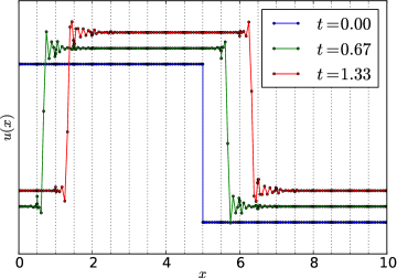
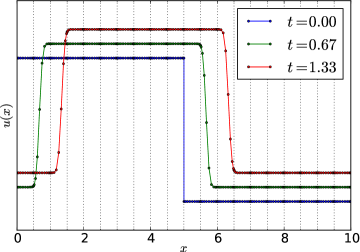
The first set of results we would like to discuss relates to the advection equation (Section 3.1). The examples in this section examine the advection of the function $u(x):=\mathbf{1}_{[0,5)}$ over an interval $(0,10)$.

Kuzmin et al. [40] suggest that the advection equation is particularly suited to testing shock capturing schemes for two reasons: First, because it is the simplest PDE that can sustain a discontinuous solution, so that the behavior of the method can be observed in a well-understood setting, isolated from other characteristics and nonlinear effects. Second, because discontinuities in it are not self-steepening, in analogy to contact discontinuities in the Euler equations, it makes a challenging example to be treated with artificial viscosity: Once a discontinuity is unduly smeared by viscosity, nothing will return it to its former, sharp shape.

Figure 6(a) displays the behavior of the unmodified discontinuous Galerkin method as described in Section 3.1. As expected, a strong Gibbs-type overshoot is observed, although it is worth noting that the used upwind fluxes already provide enough dissipation of high-frequency modes to prevent the solution from becoming useless. This example, and all examples that follow in this subsection, were run at polynomial degree $N=10$ on a discretization using $K=20$ elements.

Next, Figure 6(b) displays the result of the same calculation once the artificial viscosity machinery as described above is enabled. Discontinuities are resolved within eight points, i.e. within less than one element (containing $N_{p}=11$ points) and have no visible overshoots. (Note that as an expected consequence of the clustering of the nodes towards element edges, points appear spaced closer together where the discontinuity touches an element boundary.) Element boundaries are shown as dashed lines for orientation. Figure 6(b) displays the solution after only a brief amount of simulation time has passed. It turns out that the solution–at least visually–settles into its final form and does not change much even after a large number of round-trips. The steepness of the solution is retained as in Figure 6(b), and the number of points that are required to resolve the discontinuity remains stable.

(a) Artificial viscosity activations vs. time, in a discontinuous advection calculation.

(b) Adaptively found time step vs. step number, in a discontinuous advection calculation.

Figure 7: Interaction of the shock-capturing artificial viscosity with the time discretization.

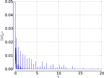
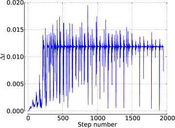
Figure 7(a) sheds a new light on this “settling” observation and the observed increased sensitivity of the detector near element boundaries that was discussed above. It shows the maximum viscosity $\|\nu\|_{L^{\infty}}$ found anywhere on the domain, graphed versus simulation time. If the observation of “brief-settling-then-steady-state” were entirely true, then one would observe no sensor activations whatsoever after “settling” has occurred. This is not what is observed here. Instead, one sees a slowly decaying train of viscosity activation spikes. It turns out that each of these spikes coincides with a discontinuity crossing an element boundary. This again confirms the observation that the detection scheme is inhomogeneous in space, i.e. it judges solution smoothness differently depending on whether a discontinuity is located in the interior of an element or at its boundary. Since the sensor is only exposed to the non-smoothness for very short periods at a time, according to Figure 7(a) it takes considerable time ($t\gtrapprox 12$ in the example) and a number of viscosity “spikes” until a profile is achieved that does not trip even the overly sensitive version of the detector. It is to be expected that the final profile is twice smoother than would be required if the oversensitivity did not exist.

As a last observation on the behavior of the method on this exceedingly simple problem, we would like to examine its interaction with the adaptive time stepper. The examples were computed using the well-known embedded Runge-Kutta method of third order by Bogacki and Shampine [8] (“ode23” in Matlab). 7(b) shows the adaptively-chosen time step $\Delta t$ as a function of the step number. The stable advective time step is clearly visible, as is the initial “settling” period discussed above, along with a variety of time step reductions occurring along the way. Some of these coincide with element transitions of discontinuities, but the situation is more ambiguous (and noisier) than in the case of viscosity activations. The figure does make one thing amply clear, however: an artificial-viscosity-based shock capturing scheme using explicit time stepping must use time step adaptivity, or it will not be competitive.

6.2 Waves: Shock Spreading and Spurious Coupling

The next, more complicated problem for which we examine the behavior of the proposed artificial viscosity is the wave equation, described in Section 3.2.

(a) EOC for the wave equation with a discontinuous initial condition without artificial viscosity.

(b) EOC for the wave equation with a discontinuous initial condition with artificial viscosity.

Figure 8: Empirical order of convergence for the wave equation with discontinuous initial conditions.

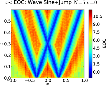
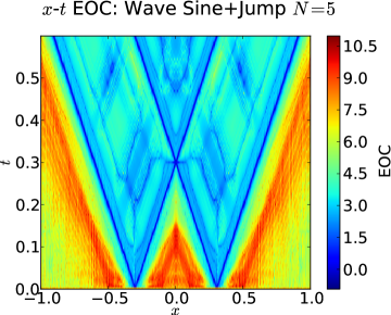
We would like to set the stage for our experimental results by considering the context of recent work by Cockburn and Guzmán [12], who show (under a number of additional assumptions) that for a DG computation of a linear advection equation at second order using a second-order total-variation-diminishing (TVD) time discretization, pollution of the numerical solution by the shock by time $T$ stays localized to an area of size $O(\sqrt{hT})$ ahead of and an area of size $O(\sqrt[3]{Th^{2}})$ behind the discontinuity. Although they only show this for a scalar advection equation, the wave equation (3.1) and its discretization may be transformed into two decoupled advection equations, and hence the result applies in this case as well.

We will study the pollution of the solution by examining its pointwise empirical order of convergence to the known analytic solution in space and time, starting from the initial condition

$$u(x,0)=2+\cos(5\pi x)+4\cdot\mathbf{1}_{[-0.3,0.3]}(x),\qquad v(x,0)=0,$$

subject to Neumann boundary conditions, on a domain $\Omega=(-1,1)$ up to a final time $T=0.6$, with a wave speed $c=1$.

Figure 8 shows the resulting convergence plots, obtained with and without artificial viscosity. As expected through the work of Cockburn and Guzmán [12], the inviscid DG scheme of Figure 8(a) achieves full convergence away from the discontinuities, but also shows a slowly-growing zone of non-convergence near the discontinuities, again matching predictions.

Unfortunately, results are not as favorable once artificial viscosity starts to act on the scheme. Outside the region that interacts with the discontinuities, convergence is roughly as before. However inside the interacting regions, convergence does improve again away from the discontinuity, but it does not recover the full order of the scheme. This reduction in order is in line with results obtained for finite-difference solutions downstream of a slightly viscous shock by Efraimsson and Kreiss [21] (see also [38]). The observation further underscores the importance of the wave equation as a test example for shock capturing schemes. Once the PDE is rewritten in as a system of first-order conservation laws, the single added viscosity of (3.1) induces a cross-coupling that appears to destroy accuracy.

Note that such behavior cannot be observed in the advection equation, or, generally, any purely scalar conservation law, since these equations have only one characteristic wave, and hence the pollution caused by the artificial viscosity cannot spread, but propagates along with the solution. This might lead one to suggest an obvious “fix” for the issue: The first-order system (i.e. the left-hand side of 3.1) can easily be transformed into characteristic variables, where it takes the form of two advection equations that only couple at the boundary, such that the issue disappears [49]. As we have already discussed, proposing this is as a general remedy is however a bit disingenuous, as it cannot work properly in multiple dimensions. Another idea that one might have to try and avoid the reduction in accuracy is to use separate viscosities for each of the variables. According to our experiments, this does not help, as the cross-coupling of the system persists.

Next, it seems unlikely that this problem is specific to the artificial viscosity constructed in this article, or to discontinuous Galerkin methods, for that matter. It should be investigated whether all artificial viscosity schemes proposed so far in the literature suffer from this shortcoming.

6.3 Euler’s Equations

In this section, we will carefully examine the behavior of the artificial viscosity method introduced above on Euler’s equations of gas dynamics, starting with the classical exact solution of the Riemann problem given by Sod [53] as the first example.

(a) $L^{2}$-projected exact and approximate numerical solutions of Sod’s problem for polynomial degree $N=5$ in $K=80$ elements.

(b) Space-time diagram of the empirical order of convergence for Sod’s problem, computed with artificial viscosity.

Figure 9: Sod’s problem with artificial viscosity: solution and $x$-$t$ convergence.

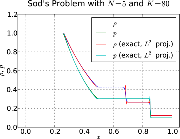
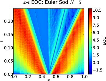
Figure 9(a) shows computational results, again at polynomial degree $N=5$ on $K=80$ elements, in direct comparison with the ($L^{2}$ projection of) the exact solution, for the density $\rho$ and the pressure $p$, at the final time $T=0.25$ of the computation.

While the figure above gives an impression of the desired solution and a first impression of the performance of the method, it is perhaps more enlightening to examine an analog to the the convergence in space and time of Figure 8 in the gas dynamics setting. Figure 9(b) provides this. As above, the computation was carried out at polynomial degree $N=5$, at a variety of mesh resolutions ranging from $K=20$ to $320$ elements across the domain. Like in the linear case, convergence away from the shock region is good, while in the central, shock-interacting ‘fan’, it hardly exceeds order 1. In particular, it is worth noting that convergence along the profile of the smooth rarefaction wave is also no better than order 1. Given the results obtained for the wave equation, this is not very surprising, and it confirms that the issues observed on linear problems persist in the nonlinear case.

(a) Close-up view of the contact discontinuity in Figure 9(a) at low and high numerical resolutions. Interpolation nodes for the low-resolution case are shown as dots.

(b) Extreme close-up view of the tip of the contact discontinuity in Figure 10(a), at low and high numerical resolutions.

Figure 10: Element-scale oscillation exhibited by the artificial viscosity scheme.

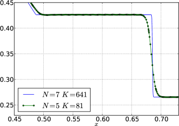
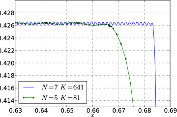
A closer look at the numerical solutions in the poorly-converged region of 9(b) offers a revealing insight, shown in Figure 10 for a high-resolution case ($N=7$, $K=641$) and a low-resolution case ($N=5$, $K=81$). On the constant parts of the solution to the Riemann problem, we observe small “wrinkles”. Figure 10(a) provides a sense of scale, while the extreme close-up of Figure 10(b) shows the phenomenon in detail. In both the high- and the low-resolution case, the oscillation’s wave length roughly agrees with the size of an element. Further, it is remarkable that the magnitude of the oscillation appears to grow, rather than shrink, with increased resolution, which seems to indicate that convergence below the margin provided for by the oscillation might not occur. (Convergence will be examined in some detail below.) The phenomenon is observed on all constant areas that are inside the fan of characteristics emanating from the shock at time $t=0$. So far, we do not understand the cause of this phenomenon, nor is it known whether there is a connection between these wrinkles and the reduced convergence observed in Section 6.2. One might speculate that, again, the detector’s spatial inhomogeneity is to blame. While we are as yet unsure of the source of the phenomenon, we would like to note that post-shock oscillations of this nature have been observed and studied even in schemes that do not use element-based decompositions [2].

	$N=4$	$N=5$	$N=7$	$N=9$	EOC
$h/1$	$9.982\cdot 10^{-3}$	$7.934\cdot 10^{-3}$	$6.522\cdot 10^{-3}$	$5.567\cdot 10^{-3}$	0.70
$h/2$	$5.442\cdot 10^{-3}$	$4.231\cdot 10^{-3}$	$3.395\cdot 10^{-3}$	$2.921\cdot 10^{-3}$	0.75
$h/4$	$2.945\cdot 10^{-3}$	$2.219\cdot 10^{-3}$	$1.778\cdot 10^{-3}$	$1.568\cdot 10^{-3}$	0.76
$h/8$	$1.548\cdot 10^{-3}$	$1.166\cdot 10^{-3}$	$9.488\cdot 10^{-4}$	$8.329\cdot 10^{-4}$	0.74
$h/16$	$8.087\cdot 10^{-4}$	$6.006\cdot 10^{-4}$	$5.121\cdot 10^{-4}$	$4.598\cdot 10^{-4}$	0.66
$h/32$	$4.207\cdot 10^{-4}$	$3.111\cdot 10^{-4}$	$2.806\cdot 10^{-4}$	—	0.69
EOC	0.93	0.95	0.92	0.92

Table 1: $L^{1}$ error and convergence data for the Sod problem of the Euler equations of gas dynamics. “EOC” stands for the empirical order of convergence, obtained as a least-squares fit to the data.

Beyond the spot testing conducted so far, we have also carried out a more comprehensive convergence study on the Euler equations applied to the Sod problem. The raw $L^{1}$ error data as well as empirical convergence order results obtained from least-squares fits are shown in Table 1. The data was gathered at a variety of polynomial degrees $N$ and with $K=20$ elements at the coarsest level, with uniform refinements thereafter. The data seems to support about a full order of convergence in $h=1/K$. No improvement in convergence occurs as the order is increased. Further, the data supports less than a full order of convergence in $N$, indicating that an addition of elemental resolution at present is a more effective way of getting a more accurate solution than increasing the size of the local approximation spaces, especially considering that the computational complexity grows superlinearly in $N$. At the resolutions examined, the influence of the oscillations (“wrinkles”) observed above does not appear to have contributed a significant part of the error–given their observed behavior in response to resolution changes, they would likely have represented a “bottom” to convergence at some fixed error magnitude. That issue aside, the observed convergence data appears to be as good as one might reasonably expect. While convergence of higher order would of course be desirable, the method as it presently stands is not designed to be able to achieve this. Through some experiments on polynomials, we have reason to believe that convergence of order one in $N$ is achievable and thereby a goal for future research.

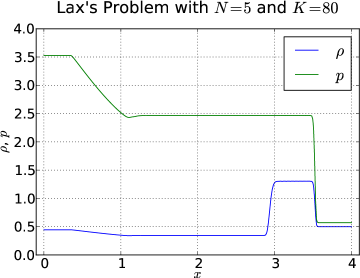
In addition to the problem of Sod [53], which has furnished the basis for all tests so far, we have also conducted tests using other available solutions for the Euler equations. One such solution that is rather similar to the Sod problem is that of Lax [42] in that it also originates from a Riemann problem. Figure 11(a) demonstrates that the scheme can successfully compute a correct solution to the problem. Lax’s problem prominently features a contact discontinuity, which is prone to smearing, as was discussed above. The contact discontinuity in the figure appears somewhat more smeared than the Sod contact discontinuity at a similar scale.

(a) Approximate numerical solution for density and pressure of Lax’s problem for polynomial degree $N=5$ in $K=80$ elements.

(b) Approximate numerical solution for density and pressure of a shock-wave interaction problem for polynomial degree $N=5$ in $K=80$ elements.

Figure 11: Solutions of classical test problems for the Euler equations using the artificial viscosity scheme.

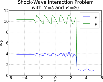
A further basic benchmark test for the method applied to the one-dimensional Euler equations was proposed by Shu and Osher [51, Example 8] to highlight the need for high-order methods in properly capturing the interaction of shocks with smooth wave-like features. Considering the gathered convergence data, we cannot claim that the method is of high order away from discontinuities once such areas enter the domain of influence of a location where artificial viscosity was applied. Nonetheless, it is still instructive to see that the method is capable of keeping the computation stable and delivering a correct result at least in the “picture norm”, as evidenced by Figure 11(b). This example is commonly considered challenging, and it is encouraging that the method is able to stabilize the computation and give a meaningful result without excessive smearing.

As a final validation of the detector’s design on the Euler equations, it is important to examine whether it will recognize smooth solutions and leave them untouched, preserving high-order accuracy. We have tested this using the smooth isentropic vortex test case of Zhou and Wei [64] with the result that as soon as sufficient resolution is available, the detector does not activate anywhere at any time during the solution process.

7 Conclusions and Future Work

What sets the shock detection method of this article apart is its focus on reliable scaling, with a further emphasis on explicit, local, GPU-suited calculation in the context of discontinuous Galerkin methods. Despite a focus on remaining issues, we contend that in this niche the method is reasonably successful. Its construction introduces several new concepts, such as a more precise interpretation of the correspondence between polynomial decay and smoothness, as well as methods like skyline pessimization, baseline decay, and $P^{1}$ viscosity smoothing.

The study of the method’s behavior on simple problems (such as linear waves and transport) was–in our opinion–quite revealing, and it should be investigated in how far other shock capturing methods are susceptible to the same problems.

On more complicated nonlinear problems, results were, in our estimation, encouraging. For example, the method manages to stabilize the computation of the shock-wave-interaction example and other important benchmarks, without introducing excessive smoothness. Further investigation, using the rich pool of tests available in the shock capturing literature [61, 3, 52, 54] will doubtlessly give further insight into the method’s strengths and weaknesses as well as help to further improve it. In addition, we have been exploring the necessities and pitfalls involved in generalizing the method to multiple dimensions. Initial tests showed promising results, which we will report in a future article.

References

- Arnold et al. [2002] D. N. Arnold, F. Brezzi, B. Cockburn, and L. D. Marini. Unified Analysis of Discontinuous Galerkin Methods for Elliptic Problems. SIAM Journal on Numerical Analysis, 39(5):1749–1779, 2002. doi: 10.1137/S0036142901384162.
- Arora and Roe [1997] M. Arora and P. L. Roe. On postshock oscillations due to shock capturing schemes in unsteady flows. Journal of Computational Physics, 130(1):25 – 40, 1997. ISSN 0021-9991. doi: 10.1006/jcph.1996.5534.
- ASC Flash Center [2009] ASC Flash Center. Flash user’s guide, version 3.2. Technical report, University of Chicago, 2009. URL http://flash.uchicago.edu/. Retrieved Apr 11, 2010.
- Barter and Darmofal [2010] G. E. Barter and D. L. Darmofal. Shock capturing with PDE-based artificial viscosity for DGFEM: Part I. Formulation. Journal of Computational Physics, 229(5):1810 – 1827, 2010. doi: 10.1016/j.jcp.2009.11.010.
- Bassi and Rebay [1994] F. Bassi and S. Rebay. Accurate 2D Euler computations by means of a high order discontinuous finite element method. In XIVth ICN MFD, Bangalore, India, July 1994. Springer.
- Bassi et al. [1997] F. Bassi, S. Rebay, G. Mariotti, S. Pedinotti, and M. Savini. A high-order accurate discontinuous finite element method for inviscid and viscous turbomachinery flows. In R. Decuypere and G. Dibelius, editors, 2nd European Conference on Turbomachinery Fluid Dynamics and Thermodynamics, page 99–108, Antwerpen, Belgium, March 1997. Technologisch Instituut.
- Bell and Garland [2008] N. Bell and M. Garland. Efficient Sparse Matrix-Vector Multiplication on CUDA. NVIDIA Technical Report NVR-2008-004, NVIDIA Corporation, December 2008.
- Bogacki and Shampine [1989] P. Bogacki and L. F. Shampine. A 3(2) pair of Runge-Kutta formulas. Applied Mathematics Letters, 2(4):321 – 325, 1989. doi: 10.1016/0893-9659(89)90079-7.
- Borwein and Erdélyi [1995] P. Borwein and T. Erdélyi. Polynomials and Polynomial Inequalities. Springer, first edition, September 1995. ISBN 0387945091.
- Burbeau et al. [2001] A. Burbeau, P. Sagaut, and C. H. Bruneau. A Problem-Independent Limiter for High-Order Runge-Kutta Discontinuous Galerkin Methods. Journal of Computational Physics, 169(1):111 – 150, 2001. doi: 10.1006/jcph.2001.6718.
- Burman [2007] E. Burman. On nonlinear artificial viscosity, discrete maximum principle and hyperbolic conservation laws. BIT Numerical Mathematics, 47(4):715–733, 2007. doi: 10.1007/s10543-007-0147-7.
- Cockburn and Guzmán [2008] B. Cockburn and J. Guzmán. Error estimates for the Runge–Kutta discontinuous Galerkin method for the transport equation with discontinuous initial data. SIAM Journal on Numerical Analysis, 46(3):1364–1398, 2008. doi: 10.1137/060668936.
- Cockburn and Shu [1989] B. Cockburn and C. Shu. TVB Runge-Kutta local projection discontinuous Galerkin finite element method for conservation laws II: general framework. Mathematics of Computation, 52(186):411–435, 1989. doi: 10.2307/2008474.
- Cockburn and Shu [1998] B. Cockburn and C.-W. Shu. The Runge-Kutta Discontinuous Galerkin Method for Conservation Laws V: Multidimensional Systems. Journal of Computational Physics, 141(2):199 – 224, 1998. doi: 10.1006/jcph.1998.5892.
- Cockburn et al. [1989] B. Cockburn, S.-Y. Lin, and C.-W. Shu. TVB Runge-Kutta local projection discontinuous Galerkin finite element method for conservation laws III: One-dimensional systems. Journal of Computational Physics, 84(1):90 – 113, 1989. doi: 10.1016/0021-9991(89)90183-6.
- Cockburn et al. [1990] B. Cockburn, S. Hou, and C.-W. Shu. The Runge-Kutta Local Projection Discontinuous Galerkin Finite Element Method for Conservation Laws. IV: The Multidimensional Case. Mathematics of Computation, 54(190):545–581, 1990. doi: 10.2307/2008501.
- Davis [1963] P. Davis. Interpolation and approximation. Blaisdell Pub. Co., 1963.
- Dolejsí et al. [2003] V. Dolejsí, M. Feistauer, and C. Schwab. On some aspects of the discontinuous Galerkin finite element method for conservation laws. Mathematics and Computers in Simulation, 61(3-6):333 – 346, 2003. doi: 10.1016/S0378-4754(02)00087-3.
- Dormand and Prince [1980] J. R. Dormand and P. J. Prince. A family of embedded Runge-Kutta formulae. Journal of Computational and Applied Mathematics, 6(1):19 – 26, 1980. doi: 10.1016/0771-050X(80)90013-3.
- Dubiner [1991] M. Dubiner. Spectral methods on triangles and other domains. Journal of Scientific Computing, 6:345–390, December 1991. doi: 10.1007/BF01060030.
- Efraimsson and Kreiss [1999] G. Efraimsson and G. Kreiss. A remark on numerical errors downstream of slightly viscous shocks. SIAM Journal on Numerical Analysis, 36(3):853–863, 1999. doi: http://dx.doi.org/10.1137/S0036142996313282.
- Ern et al. [2009] A. Ern, A. Stephansen, and P. Zunino. A discontinuous Galerkin method with weighted averages for advection-diffusion equations with locally small and anisotropic diffusivity. IMA Journal of Numerical Analysis, 29(2):235, 2009. doi: 10.1093/imanum/drm050.
- Feistauer and Kučera [2007] M. Feistauer and V. Kučera. On a robust discontinuous Galerkin technique for the solution of compressible flow. Journal of Computational Physics, 224(1):208 – 221, 2007. doi: 10.1016/j.jcp.2007.01.035.
- Flaherty et al. [1997] J. E. Flaherty, R. M. Loy, M. S. Shephard, B. K. Szymanski, J. D. Teresco, and L. H. Ziantz. Adaptive local refinement with octree load balancing for the parallel solution of three-dimensional conservation laws. Journal of Parallel and Distributed Computing, 47(2):139 – 152, 1997. doi: 10.1006/jpdc.1997.1412.
- Gottlieb and Shu [1997] D. Gottlieb and C.-W. Shu. On the gibbs phenomenon and its resolution. SIAM Review, 39(4):644–668, 1997. doi: 10.1137/S0036144596301390. URL http://link.aip.org/link/?SIR/39/644/1.
- Gottlieb et al. [2011] S. Gottlieb, D. Ketcheson, and C. Shu. Strong Stability Preserving Time Discretizations. World Scientific, 2011.
- Gresho and Lee [1981] P. M. Gresho and R. L. Lee. Don’t suppress the wiggles–they’re telling you something! Computers & Fluids, 9(2):223 – 253, 1981. ISSN 0045-7930. doi: 10.1016/0045-7930(81)90026-8.
- Guermond and Pasquetti [2008] J.-L. Guermond and R. Pasquetti. Entropy-based nonlinear viscosity for Fourier approximations of conservation laws. Comptes Rendus Mathematique, 346(13-14):801 – 806, 2008. doi: 10.1016/j.crma.2008.05.013.
- Harris [2007] M. Harris. Optimizing parallel reduction in CUDA. Technical report, Nvidia Corporation, Santa Clara, CA, 2007. URL http://developer.download.nvidia.com/compute/cuda/1_1/Website/projects/%reduction/doc/reduction.pdf. Retrieved Apr 14, 2010.
- Hartmann [2006] R. Hartmann. Adaptive discontinuous Galerkin methods with shock-capturing for the compressible Navier-Stokes equations. International Journal for Numerical Methods in Fluids, 51(9):1131–1156, 2006. doi: 10.1002/fld.1134.
- Hesthaven and Warburton [2007] J. S. Hesthaven and T. Warburton. Nodal Discontinuous Galerkin Methods: Algorithms, Analysis, and Applications. Springer, first edition, November 2007. ISBN 0387720650.
- Houston and Süli [2005] P. Houston and E. Süli. A note on the design of hp-adaptive finite element methods for elliptic partial differential equations. Computer Methods in Applied Mechanics and Engineering, 194(2-5):229 – 243, 2005. ISSN 0045-7825. doi: 10.1016/j.cma.2004.04.009.
- Jaffre et al. [1995] J. Jaffre, C. Johnson, and A. Szepessy. Convergence of the discontinuous Galerkin finite element method for hyperbolic conservation laws. Math. Models Methods Appl. Sci., 5(3):367–386, 1995.
- John and Schmeyer [2008] V. John and E. Schmeyer. Finite element methods for time-dependent convection–diffusion–reaction equations with small diffusion. Computer Methods in Applied Mechanics and Engineering, 198(3-4):475–494, 2008. doi: 10.1016/j.cma.2008.08.016.
- Kirby and Sherwin [2006] R. M. Kirby and S. J. Sherwin. Stabilisation of spectral/hp element methods through spectral vanishing viscosity: Application to fluid mechanics modelling. Computer Methods in Applied Mechanics and Engineering, 195(23-24):3128 – 3144, 2006. doi: 10.1016/j.cma.2004.09.019.
- Klöckner et al. [2009] A. Klöckner, T. Warburton, J. Bridge, and J. Hesthaven. Nodal discontinuous Galerkin methods on graphics processors. J. Comp. Phys., 228:7863–7882, 2009. doi: 10.1016/j.jcp.2009.06.041.
- Koornwinder [1975] T. Koornwinder. Two-variable analogues of the classical orthogonal polynomials. Theory and Applications of Special Functions, pages 435–495, 1975.
- Kreiss et al. [2001] G. Kreiss, G. Efraimsson, and J. Nordström. Elimination of first order errors in shock calculations. SIAM Journal on Numerical Analysis, 38(6):1986–1998, 2001. doi: http://dx.doi.org/10.1137/S0036142998349412.
- Krivodonova [2007] L. Krivodonova. Limiters for high-order discontinuous galerkin methods. Journal of Computational Physics, 226(1):879–896, 2007. doi: 10.1016/j.jcp.2007.05.011.
- Kuzmin et al. [2005] D. Kuzmin, R. Löhner, and S. Turek. Flux-corrected transport. Springer, 2005.
- Lapidus [1967] A. Lapidus. A detached shock calculation by second-order finite differences. Journal of Computational Physics, 2(2):154 – 177, 1967. doi: 10.1016/0021-9991(67)90032-0.
- Lax [1954] P. D. Lax. Weak solutions of nonlinear hyperbolic equations and their numerical computation. Communications on Pure and Applied Mathematics, 7(1):159–193, 1954. doi: 10.1002/cpa.3160070112.
- Lesaint and Raviart [1974] P. Lesaint and P. Raviart. On a finite element method for solving the neutron transport equation. Mathematical aspects of finite elements in partial differential equations, pages 89–123, 1974.
- Lörcher et al. [2008] F. Lörcher, G. Gassner, and C.-D. Munz. An explicit discontinuous Galerkin scheme with local time-stepping for general unsteady diffusion equations. J. Comp. Phys., 227:5649–5670, 2008. doi: 10.1016/j.jcp.2008.02.015.
- Mavriplis [1994] C. Mavriplis. Adaptive mesh strategies for the spectral element method. Computer Methods in Applied Mechanics and Engineering, 116(1-4):77 – 86, 1994. doi: 10.1016/S0045-7825(94)80010-3.
- Persson and Peraire [2006] P. Persson and J. Peraire. Sub-Cell Shock Capturing for Discontinuous Galerkin Methods. In Proc. of the 44th AIAA Aerospace Sciences Meeting and Exhibit, volume 112, 2006.
- Proft and Rivière [2009] J. Proft and B. Rivière. Discontinuous Galerkin Methods For Convection-Diffusion Equations For Varying And Vanishing Diffusivity. Int. J. Num. Anal. Mod., 6(4):533–561, 2009.
- Reed and Hill [1973] W. H. Reed and T. R. Hill. Triangular mesh methods for the neutron transport equation. Technical report, Los Alamos Scientific Laboratory, Los Alamos, 1973.
- Rieper [2010] F. Rieper. On the dissipation mechanism of upwind-schemes in the low Mach number regime: A comparison between Roe and HLL. Journal of Computational Physics, 229(2):221–232, 2010. doi: 10.1016/j.jcp.2009.09.043.
- Shu [1988] C. Shu. Total-variation-diminishing time discretizations. SIAM Journal on Scientific and Statistical Computing, 9:1073, 1988. doi: 10.1137/0909073.
- Shu and Osher [1989] C.-W. Shu and S. Osher. Efficient implementation of essentially non-oscillatory shock-capturing schemes, ii. Journal of Computational Physics, 83(1):32 – 78, 1989. doi: 10.1016/0021-9991(89)90222-2.
- Slater et al. [2009] J. Slater, J. Dudek, K. Tatum, et al. The NPARC Alliance Verification and Validation Archive., 2009. URL http://www.grc.nasa.gov/WWW/wind/valid/archive.html. Retrieved Apr 11, 2010.
- Sod [1978] G. A. Sod. A survey of several finite difference methods for systems of nonlinear hyperbolic conservation laws. Journal of Computational Physics, 27(1):1 – 31, 1978. doi: 10.1016/0021-9991(78)90023-2.
- Stone [2009] J. M. Stone. Athena test archive, 2009. URL http://www.astro.princeton.edu/~jstone/tests/. Retrieved Apr 11, 2010.
- Tadmor [1989] E. Tadmor. Convergence of spectral methods for nonlinear conservation laws. SIAM Journal on Numerical Analysis, 26(1):30–44, 1989. doi: 10.1137/0726003.
- Tu and Aliabadi [2005] S. Tu and S. Aliabadi. A slope limiting procedure in discontinuous Galerkin finite element method for gasdynamics applications. International Journal of Numerical Analysis and Modeling, 2(2):163–178, 2005.
- von Neumann and Richtmyer [1950] J. von Neumann and R. Richtmyer. A method for the numerical calculation of hydrodynamic shocks. Journal of Applied Physics, 21:232–237, 1950. doi: 10.1063/1.1699639.
- Warburton [2006] T. Warburton. An explicit construction of interpolation nodes on the simplex. J. Eng. Math., 56:247–262, 2006. doi: 10.1007/s10665-006-9086-6.
- Warburton and Hagstrom [2008] T. Warburton and T. Hagstrom. Taming the CFL Number for Discontinuous Galerkin Methods on Structured Meshes. SIAM J. Num. Anal., 46:3151–3180, 2008. doi: 10.1137/060672601.
- Warburton et al. [1999] T. Warburton, I. Lomtev, Y. Du, S. Sherwin, and G. Karniadakis. Galerkin and discontinuous Galerkin spectral/hp methods. Computer Methods in Applied Mechanics and Engineering, 175(3-4):343 – 359, 1999. doi: 10.1016/S0045-7825(98)00360-0.
- Woodward and Colella [1984] P. Woodward and P. Colella. The numerical simulation of two-dimensional fluid flow with strong shocks. Journal of Computational Physics, 54(1):115–173, 1984. doi: 10.1016/0021-9991(84)90142-6.
- Xu et al. [2009] Z. Xu, Y. Liu, and C.-W. Shu. Hierarchical reconstruction for discontinuous Galerkin methods on unstructured grids with a WENO-type linear reconstruction and partial neighboring cells. Journal of Computational Physics, 228(6):2194 – 2212, 2009. doi: 10.1016/j.jcp.2008.11.025.
- Xu et al. [2010] Z. Xu, J. Xu, and C.-W. Shu. A high order adaptive finite element method for solving nonlinear hyperbolic conservation laws. Technical Report 2010-14, Scientific Computing Group, Brown University, Providence, RI, USA, Apr. 2010.
- Zhou and Wei [2003] Y. C. Zhou and G. W. Wei. High resolution conjugate filters for the simulation of flows. Journal of Computational Physics, 189(1):159 – 179, 2003. doi: 10.1016/S0021-9991(03)00206-7.