A large-deviation approach to space-time chaos

Abstract

In this Letter we show that the analysis of Lyapunov-exponents fluctuations contributes to deepen our understanding of high-dimensional chaos. This is achieved by introducing a Gaussian approximation for the large deviation function that quantifies the fluctuation probability. More precisely, a diffusion matrix $\bf D$ (a dynamical invariant itself) is measured and analysed in terms of its principal components. The application of this method to three (conservative, as well as dissipative) models, allows: (i) quantifying the strength of the effective interactions among the different degrees of freedom; (ii) unveiling microscopic constraints such as those associated to a symplectic structure; (iii) checking the hyperbolicity of the dynamics.

Introduction - There are two complementary reasons to investigate the links between statistical mechanics and space-time chaos. On the one hand, (equilibrium) statistical mechanics provides an effective framework to describe the evolution of nonlinear systems. This is achieved through the introduction of the so-called thermodynamic formalism ruelle and is based on a suitable partition of the phase-space and the consequent interpretation of the time-axis as an additional spatial direction. This approach proved to be very effective in the characterization of low-dimensional systems and has contributed to establish, e.g., the relationship between Lyapunov exponents on the one side and fractal dimension or the Kolmogorov-Sinai entropy, on the other book . A generalization of the approach to spatially extended systems is formally possible, but almost unfeasible, because of the difficulty to construct appropriate phase-space partitions politi . On the other hand, a detailed understanding of high-dimensional chaos can help bridging the gap between microscopic and macroscopic evolution, thereby laying the foundations for a dynamical theory of (non)equilibrium statistical mechanics. In this perspective, the estimation of a suitable large deviation function appears to be the most promising strategy. This idea proved already fruitful in the context of a stochastic dynamics, where some exact calculations have been performed in simple but non-trivial models of interacting particles derrida ; new . In the context of chaotic systems, instead, this approach is the core of the Gallavotti-Cohen fluctuation theorem gallavotti , that is proved under the hypothesis that, in the thermodynamic limit, the evolution of typical dynamical systems is effectively hyperbolic.

In this Letter, we propose an approach that can contribute to make progress along both directions, without introducing any assumption of the underlying dynamics. More precisely, we suggest to study the fluctuations of the Lyapunov exponents (LEs) along the lines of the multifractal theory book . One of the advantages of dealing with LEs and their fluctuations (in the long-time limit) is that they are dynamical invariants, i.e. they are independent of the parametrization of the phase space. An exact implementation in generic nonlinear models is out of question. Nevertheless, here we show that useful information can be extracted by working within the Gaussian approximation. For instance, we show that the (cross)correlations among all pairs of LEs and, in particular, their scaling behavior with the system size allows estimating the strength of the effective interactions that spontaneously emerge among the various degrees of freedom. Notice that our analysis goes beyond the usual extensivity assessment of space-time chaos, that is linked to the existence of a limit Lyapunov spectrum. In fact, we will see that the fluctuations of a chain of contiguous non-interacting systems are substantially different from those of a typical chain of interacting systems. Finally, our approach allows testing the hyperbolicity of the underlying dynamics, by: (i) comparing the results obtained for different defintions of the Lyapunov exponents, (ii) testing phenomena like the dominance of Oseledec splitting dos , and (iii) quantifying dimension variability lai .

Theory - Let $\Lambda_{i}(\tau)$ denote the $i$th expansion factor over a time $\tau$ in tangent space. The rate $\lambda_{i}=\Lambda_{i}(\tau)/\tau$ is the so-called finite-time Lyapunov exponent (FTLE), which, in the infinite-time limit, converges to the LE $\overline{\lambda}_{i}$ (here and in the following, overlines denote time averages). For finite $\tau$, FTLEs fluctuate around the asymptotic values. The theory of large deviations suggests that, in the long-time limit, the probability distribution $P(\boldsymbol{\lambda},\tau)$ (where $\boldsymbol{\lambda}=\{\lambda_{1},\lambda_{2},\ldots,\lambda_{N}\}$ and $N$ is the number of degrees of freedom) scales with $\tau$ as

$$P(\boldsymbol{\lambda},\tau)\underset{\tau\to\infty}{\propto}{\rm e}^{-S(\boldsymbol{\lambda})\tau}$$ (1)

where $S(\boldsymbol{\lambda})$ is the positive-definite large deviation function whose minimum (equal to zero) is achieved in correspondence of the LEs $\overline{\lambda}_{i}$. $S$ has been mostly studied in contexts where $\boldsymbol{\lambda}$ reduces to a scalar variable $\lambda$, as it happens for low-dimensional chaos, where it is known that $S(\lambda)$ is itself a dynamical invariant book . This is because FTLE fluctuations originate from passages of a chaotic trajectory in the vicinity of periodic orbits with different stability properties. There is no reason to doubt that dynamical invariance is lost upon increasing the dimensionality of the phase-space.

If a system is the Cartesian product of uncoupled variables, $S$ is the sum of functions, each dependent on a single $\lambda_{i}$, but interactions bring new terms. Although determining $S$ is too ambitious a task, relevant features can be uncovered by expanding it around the minimum $\overline{\boldsymbol{\lambda}}$, and retaining the first (quadratic) non-zero term,

$$S(\boldsymbol{\lambda})\approx\frac{1}{2}(\boldsymbol{\lambda}-\overline{\boldsymbol{\lambda}}){\bf Q}(\boldsymbol{\lambda}-\overline{\boldsymbol{\lambda}})^{\dagger}$$ (2)

(${\dagger}$ denotes the transpose), an approximation that is equivalent to assuming a Gaussian distribution. In practice, it is preferable to consider the symmetric matrix ${\bf D}={\bf Q}^{-1}$. In fact, the elements $D_{ij}$ can be directly determined by estimating the (linear) growth rate of the (co)variances of $(\Lambda_{i}(\tau)-\overline{\lambda}_{i}\tau)$,

$$D_{ij}=\lim_{\tau\to\infty}\left(\overline{\Lambda_{i}(\tau)\Lambda_{j}(\tau)}-\overline{\lambda}_{i}\overline{\lambda}_{j}\tau^{2}\right)/\tau.$$ (3)

There are three basic definitions of FTLEs. One can compute them:(i) by repeatedly applying the Gram-Schmidt orthogonalization procedure to a set of linearly independent perturbations (backward or Gram-Schmidt Lyapunov vectors); (ii) by performing this procedure along the negative time axis (forward Lyapunov vectors); (iii) by making reference to the covariant Lyapunov vectors ginelli . In the infinite-time limit, the three methods produce identical LEs. For finite but long times, as long as FTLE fluctuations are connected to “visits” of different periodic orbits, the three defintions should be again equivalent. In fact, we have systematically verified that the correlations computed with the methods (i) and (iii) are basically indistinguishable as soon as the diffusive asymptotic behavior sets in noteme . This result provides a first evidence of the effective hyperbolicity of the underlying dynamics. In fact, it implies that the differences induced by the presence of homoclinic tangencies are so rare that they do not affect our perturbative analysis.

The information contained in $\bf D$ can be expressed in a compact form by determining its (positive) eigenvalues $\mu_{k}$ ($k=1,N$), which represent the fluctuation amplitudes along the most prominent directions. Some of the eigenvalues may turn out to vanish because of more or less hidden constraints. For instance, in the presence of a constant phase-space contraction rate, $\sum_{i}\lambda_{i}={\rm const}$ and all $\{\lambda_{i}\}$ $n$-tuples lie in a same hyperplane. As a result, one eigenvalue of $\bf D$ is equal to zero: its corresponding eigenvector is perpendicular to the hyperplane itself. Another instructive case is that of symplectic dynamics: since the LEs come in pairs whose sum is zero, the fluctuations of the negative LEs are perfectly anticorrelated with those of the positive ones, so that $D_{ij}$ has an additional symmetry $\cal S$, i.e., $D_{N+1-i,j}=D_{i,N+1-j}=-D_{ij}$. Altogether, the possible existence of zero eigenvalues reinforces the choice of studying $\bf D$ rather than its ill-defined inverse $\bf Q$. Moreover, since the matrices $\bf Q$ and $\bf D$ are diagonal in the same basis, and the eigvenvalues of $\bf Q$ are the inverse of those of $\bf D$, we can infer the scaling behavior of the former ones from that of the latter. One must simply be careful and discard the redundant variables, associated to the zero eigenvalues. In particular, since, as we shall see, $\mu_{k}\propto 1/N$, the large deviation function $S$ turns out to be proportional to the number $N$ of degrees of freedom, i.e., it is an extensive quantity.

Model analysis - We start the numerical analysis by studying a chain of Hénon maps torc92

$$x_{n}(t+1)=a-[x_{n}(t)+\varepsilon{\cal D}x_{n}(t)]^{2}+bx_{n}(t-1)\,,$$ (4)

where ${\cal D}x_{n}\equiv(x_{n-1}-2x_{n}+x_{n+1})$ is the discrete Laplacian operator. We have chosen $a=1.4$, $b=0.3$, $\varepsilon=0.025$ and used periodic boundary conditions (the same conditions have been chosen in the other models too). The results are shown in Fig. 1. In panel a) we report the self-diffusion coefficients $D_{ii}$ (see the symbols). The clean overlap of the scaled curves indicates that $D_{ii}(\rho)\approx 1/N^{0.85}$. This means that the LEs self-average in the thermodynamic limit. The singular behavior exhibited by $D_{ii}(\rho)$ for $\rho\to 1$ follows from the different scaling behavior of the first and $N$th exponent which decrease as $1/\sqrt{N}$. In Fig. 1b we plot $D_{ij}$ along the column $j=2N/5$. The off-diagonal terms decrease as $1/N$, so that the matrix $\bf D$ becomes increasingly diagonal in the thermodynamic limit. Finally, the eigenvalue spectrum $\mu_{k}$ (see Fig. 1c) decreases like $1/N$. This implies that the eigenvalues of $\bf Q$ are proportional to $N$, i.e. the large deviation function is an extensive observable. Moreover, the $1/\sigma$ singularity at $\sigma=0$ means that the leading eigenvalue $\mu_{1}$ does not decrease, i.e., there exists one direction in phase-space along which fluctuations survive even in the thermodynamic limit. The physical meaning of this feature is to be understood. Finally, the eigenvalue spectrum exhibits a remarkable and unexpected property: half of it is equal to zero. A close inspection of the whole correlation matrix reveals that this is because $\bf D$ is $\cal S$-symmetric. By further investigating the Jacobian matrix $\bf J$, we have discovered that it indeed satisfies the symplectic-like condition ${\bf J}{\bf A}{\bf J}^{\rm T}=-b{\bf A}$ (see unpu ). Unlike the similar case studied in Ref. dressler , here ${\bf A}$ is a generic antisymmetric matrix depending on $t$. Altogether, these results indicate that LEs come in pairs, such that $\overline{\lambda}_{i}+\overline{\lambda}_{N+1-i}=\ln b$.

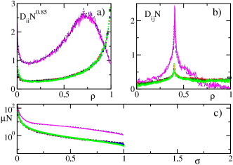
Figure 1: (Color online) Diffusion coefficients in a chain of Hénon (symbols) and symplectic (lines) maps. In all panels, squares, diamonds, plusses and circles refer to $N=40$, 80, 160, and 320 respectively, while dotted, dashed and solid lines correspond to $N=32$, 64, and 128, respectively. The results have been obtained by iterating the chain over $5\times 10^{6}$ time steps. Panel a) contains the diagonal elements, $\rho=(i-1/2)/N$; panel b) refers to the column $j=2N/5$, $\rho=i/N$; panel c) refers to the eigenvalues of $\bf D$, ordered from the largest to the smallest one, $\sigma=k/N$.

Next we have studied a chain of symplectic maps,

$$p_{n}(t+1) = p_{n}(t)+K(\sin\Delta\theta_{n+1}(t)-\sin\Delta\theta_{n}(t))$$

$$\theta_{n}(t+1) = \theta_{n}(t)+p_{n}(t+1)$$ (5)

where both $p_{n}$ and $\theta_{n}$ are defined modulus $2\pi$ and $\Delta\theta_{n}=\theta_{n}-\theta_{n-1}$. The model has been simulated for $K=4$. In Fig. 1 (see the lines), one can notice that the overall scenario is very similar to that one observed in the chain of Hénon maps, including the behavior of the diagonal elements. The major difference concerns $D_{NN}$ which, instead of decreasing faster, it now decreases slower than in the bulk.

Finally, we have considered a chain of Stuart-Landau oscillators as an example of a continuous-time dissipative system. The model can be viewed as the spatial discretization of a complex Ginzburg-Landau equation, a prototypical model of space-time chaos. The evolution equation writes

$$\dot{a}_{n}=a_{n}-(1+ic)|a_{n}|^{2}a_{n}+(1+ib)h^{-2}{\cal D}a_{n}\,.$$ (6)

We have fixed $c=3$, $b=-2$ and $h=1/2$, which corresponds to a regime of amplitude turbulence parlitz . In this model we cannot draw clear conclusions on the scaling behavior of the $\bf D$ elements, because of larger finite-size corrections (see Fig. 2). However, the eigenvalues behave quite similarly to the two previous cases: (i) the overall spectrum scales as $1/N$; (ii) the maximum eigenvalue remains finite for increasing $N$; (iii) a large fraction of the spectrum is nearly equal to zero. In this case, the singularity is due to the appearance (beyond a certain $\rho$-value) of pairs of degenerate LEs parlitz which fluctuate synchronously. Notice also the drops of the diffusion coefficient indicated by arrows 1 and 2 in Fig. 2a that are discussed below.

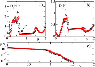
Figure 2: (Color online) Diffusion coefficients in a chain of Stuart-Landau oscillators. In all panels circles and squares refer to $N=64$ and 128, respectively. The panels are organized in the same way as in the first figure. The column reported in panel b) corresponds to $j=N/2$.

Discussion - The common property exhibited by all of the three models is the $1/N$ scaling of the eigenvalue spectrum of the diffusion matrix $\bf D$. This implies that the matrix $\bf Q$ and, thereby, the large deviation function $S$ are proportional to the number of degrees of freedom, i.e., $S$ is an extensive observable. It is interesting to notice that such a property holds in spite of the long-range correlations that are revealed by the strength of the off-diagonal terms of $\bf D$ (in all models, they provide a substantial contribution to the scaling behavior of the eigenvalues).

Next we discuss some physical implications of the structure of the large deviation function $S$. We start from the occurrence of occasional changes in the order of the FTLEs, a feature that is related to the concept of dominated Oseledec splitting dos . The splitting is dominated with index $i$ if there exists a finite $\tau_{0}$ such that $\lambda_{i}>\lambda_{i+1}$ for all $\tau>\tau_{0}$ yang . This property implies the absence of tangencies between the corresponding Oseledec subspaces identified by the $i$th vector and the subsequent one dos . The probability of order-exchanges can be inferred from the fluctuations of $\delta\lambda_{i}=\lambda_{i}-\lambda_{i+1}$. Its diffusion coefficient $K_{i}$ can be expressed in terms of the ${\bf D}$ elements, $K_{i}=D_{ii}+D_{i+1,i+1}-2D_{i,i+1}$. Since the probability of an exchange of FTLEs is equal to the probability $P_{i}^{w}$ of observing a negative $\delta\lambda_{i}$, we have, in the Gaussian approximation,

$$P_{i}^{w}\approx\frac{1}{2}{\rm erfc}\left\{(\overline{\lambda}_{i}-\overline{\lambda}_{i+1})\sqrt{\frac{\tau}{2K_{i}}}\right\},$$ (7)

where “$\rm erfc$” is the complementary error function. The analysis of the three models reveals that, in the bulk, $K_{i}$ scales always as $1/N$ (see Fig. 3) notescl . Since the distance between consecutive LEs scales also as $1/N$ (this follows from the very existence of a limit LE spectrum), one can conclude that $P_{i}^{w}\approx{\rm erfc}(c_{i}\sqrt{\tau/N})/2$ for some $c_{i}\geq 0$. This means that in the large $N$ limit, order exchanges occur with a finite probability and no dominated splitting is present. However, in the Hénon maps, at $\rho=1$, there is a gap in the Lyapunov spectrum. Therefore, since $K_{N}$ vanishes (as $1/\sqrt{N}$), the probability of order exchanges goes to zero, indicating that stable and unstable manifold are mutually transversal and the system effectively hyperbolic. The absence of a gap in the Lyapunov spectrum of the symplectic maps prevents us from drawing a similar conclusion in that model. In the Stuart-Landau chain, $P_{i}^{w}$ vanishes close to arrow “2” (see Figs. 2a and 3b), since $K_{i}=0$ (and $\overline{\lambda}_{i}\neq\overline{\lambda}_{i+1}$), thus implying that the splitting is dominated note1 . This suggests the existence of two transversal subspaces, consistently with the claim that the attractor is embedded in a supporting manifold containing the physical modes yang ; parlitz . Since the dimension of the supporting manifold is even larger than the Kaplan-Yorke dimension (equal to $0.27N$), we must conclude that the overall dynamics is not hyperbolic.

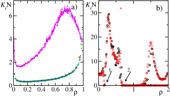
Figure 3: (Color online) Rescaled diffusion coefficients $K_{i}$ of the LE differences $\delta\lambda$ in Hénon (symbols) and symplectic (lines) maps (panel a) and Stuart-Landau oscillators (panel b), $\rho=i/N$. Same notations as in the two previous curves.

Now, we analyse the invariant measure, introducing the expansion rate $\mathcal{L}(\mathcal{D})=\sum_{i}^{\mathcal{D}}\lambda_{i}$ of a generic volume of dimension $\mathcal{D}$, over a time $\tau$. The Kaplan-Yorke dimension $\mathcal{D}_{f}$ is obtained by imposing $\overline{\mathcal{L}}(\mathcal{D}_{f})=0$ notefr . Under the assumption of small fluctuations, one can express the diffusion coefficient $\Delta_{\tau}^{\mathcal{D}}$ of $\mathcal{D}$ in terms of the analogous coefficient $\Delta^{\mathcal{L}}=\sum_{i,j}^{\mathcal{D}}D_{ij}$ of $\mathcal{L}$, by linearizing the function $\overline{\mathcal{L}}(\mathcal{D})$ around $\mathcal{D}_{f}$. This leads to $\Delta_{\tau}^{\mathcal{D}}=\Delta^{\mathcal{L}}/({\overline{\lambda}}_{\mathcal{D}_{f}})^{2}$. The dimension fluctuations $\Delta_{\varepsilon}^{\mathcal{D}}$, can now be estimated by invoking an Ansatz similar to Eq. (1) which, in the Gaussian approximation, writes $P(\mathcal{D})\propto\varepsilon^{(\mathcal{D}-\mathcal{D}_{f})^{2}/(2\Delta_{\varepsilon}^{\mathcal{D}})}$, where the box-size $\varepsilon$ must be linked to the time variable. By following Ref. grass , it is natural to assume that $\varepsilon\approx\exp(-|\overline{\lambda}_{\mathcal{D}_{f}}|\tau)$, thereby obtaining $\Delta_{\varepsilon}^{\mathcal{D}}=\Delta_{\tau}^{\mathcal{D}}\overline{\lambda}_{\mathcal{D}_{f}}=\Delta^{\mathcal{L}}/\bar{\lambda}_{\mathcal{D}_{f}}$. In the chain of Hénon maps, $\Delta_{\varepsilon}^{\mathcal{D}}\approx 0.12N$, i.e. dimension fluctuations are extensive. This implies that the naïve idea is wrong and it is necessary to build a more refined picture to refer to high-dimensional chaotic attractors.

Conclusions We have shown that a fluctuation analysis can deepen our understanding of high-dimensional chaos. The main result is the discovery of a subtle form of extensivity, i.e. the proportionality of the large deviation function to the system size. This result is nontrivial, since it arises in a context of effective long-range correlations and there are even examples of stochastic models, where the large deviation function is not extensive new . As for the discrepancy between the scaling exponent of the diagonal elements and of the eigenvalues of $\bf D$ (0.85 vs. 1) it is necessary to study larger sizes to decide whether it is due to finite-size corrections. Moreover, our approach provides a new way of investigating the hyperbolicity of a given dynamics (including dimension variability), although we are aware that the last word can be said only by going beyond the perturbative approach described in this Letter. The method introduced in Ref. kurchan to identify trajectories with unprobable stability properties, makes this perspective not so remote.

Acknolwedgements We thank S. Lepri, A. Pikovsky, H. Chaté and K. Takeuchi for useful discussions.

References

- (1) D. Ruelle, Thermodynamic formalism (Cambridge University Press, 2004).
- (2) M. Cencini, F. Cecconi, and A. Vulpiani Chaos, From simple models to complex systems, (World Scientific, Singapore 2010).
- (3) A. Politi, A. Torcini Phys. Rev. Lett. 69, 3421 (1992).
- (4) B. Derrida, J. Stat. Mech. P07023 (2007).
- (5) V. Lecomte, C. Appert-Rolland, and F. van Wijland, Phys. Rev. Lett. 95 010601 (2005).
- (6) G. Gallavotti, E.G.D. Cohen, Phys. Rev. Lett. 74, 2694 (1995).
- (7) C. Pugh, M. Shub, and A. Starkov, Bull. Am. Math. Soc. 41, 1 (2004); J. Bochi, M. Viana, Annals of Math. 161, 1423 (2005).
- (8) E.J. Kostelich et al. Physica D, 109, 81 (1997).
- (9) F. Ginelli et al. Phys. Rev. Lett. 99 130601 (2007).
- (10) A. Politi, A. Torcini, CHAOS 2, 2993 (1992).
- (11) For this reason, heavy simulations have been performed by using the fastest method (i).
- (12) P. Kuptsov, A. Politi, unpublished.
- (13) U. Dressler, Phys. Rev. A 38, 2103 (1988).
- (14) P.V. Kuptsov, U. Parlitz, Phys. Rev. E 81, 036214 (2010)
- (15) H.-L. Yang, et al., Phys. Rev. Lett. 102, 074102 (2009).
- (16) The divergence visible in Fig. 1(b) close to the diagonal implies that scales as : this term is large enough to cancel the diagonal contribution, thereby allowing to scale as .
- (17) Leaving aside (irrelevant) fractional corrections.
- (18) The same is not true close to “1”, since the vanishing of is accompanied by the presence of identical zero LEs.
- (19) P. Grassberger, R. Badii, and A. Politi, J. Stat. Phys. 51, 135 (1988).
- (20) J. Tailleur and J. Kurchan, Nature Physics 3, 203 (2007).