Nonlinear electrodynamics and CMB polarization

Abstract

Recently WMAP and BOOMERanG experiments have set stringent constraints on the polarization angle of photons propagating in an expanding universe: $\Delta\alpha=(-2.4\pm 1.9)^{\circ}$. The polarization of the Cosmic Microwave Background radiation (CMB) is reviewed in the context of nonlinear electrodynamics (NLED). We compute the polarization angle of photons propagating in a cosmological background with planar symmetry. For this purpose, we use the Pagels-Tomboulis (PT) Lagrangian density describing NLED, which has the form $L\sim(X/\Lambda^{4})^{\delta-1}\;X$, where $X=\frac{1}{4}F_{\alpha\beta}F^{\alpha\beta}$, and $\delta$ the parameter featuring the non-Maxwellian character of the PT nonlinear description of the electromagnetic interaction. After looking at the polarization components in the plane orthogonal to the ($x$)-direction of propagation of the CMB photons, the polarization angle is defined in terms of the eccentricity of the universe, a geometrical property whose evolution on cosmic time (from the last scattering surface to the present) is constrained by the strength of magnetic fields over extragalactic distances.

1 Introduction

Modifications to the standard (Maxwell) electrodynamics were proposed in the literature in order to avoid infinite physical quantities from theoretical descriptions of electromagnetic interactions. Born and Infeld [1], for instance, proposed a model in which the infinite self energy of point particles (typical of Maxwell’s electrodynamics) are removed by introducing an upper limit on the electric field strength, and by considering the electron as an electric particle with finite radius. Along this line, other models of nonlinear electrodynamics (NLED) Lagrangians were proposed by Plebanski, who also showed that Born-Infeld model satisfies physically acceptable requirements [2]. Consequences of nonlinear electrodynamics have been studied in many contexts, such a, for example, cosmological models [3], black holes and wormhole physics [4, 5], primordial magnetic fields in the Universe [9, 11, 8], gravitational baryogenesis [8], and astrophysics [12, 17].

In this paper we investigate the CMB polarization of photons described by nonlinear electrodynamics. We compute the polarization angle of photons propagating in an expanding Universe, by considering in particular cosmological models with planar symmetry. The polarization angle does depend on the parameter characterizing the nonlinearity of electrodynamics, which will be constrained by making use of the recent data from WMAP and BOOMERANG. This kind of investigations has received a lot of interest because they represent a probe of models beyond the standard model, which may violate the fundamental symmetries such as CPT and Lorentz invariance [13, 14]. In what follows we will follow the main lines of the paper on “Cosmological CPT violation, baryo/leptogenesis and CMB polarization” by Li-Xia-Li-Zhang [6].

2 Minimally coupling gravity to nonlinear electrodynamics

The action of (nonlinear) electrodynamics coupled minimally to gravity is

$$S=\frac{1}{2\kappa}\int d^{4}x\sqrt{-g}R+\frac{1}{4\pi}\int d^{4}x\sqrt{-g}L(X,Y)\,,$$ (1)

where $\kappa=8\pi G$, $L$ is the Lagrangian of nonlinear electrodynamics depending on the invariant $X=\frac{1}{4}F_{\mu\nu}F^{\mu\nu}=-2({\bf E}^{2}-{\bf B}^{2})$ and $Y=\frac{1}{4}F_{\mu\nu}\,{{}^{*}}F^{\mu\nu}$, where $F^{\mu\nu}\equiv\nabla_{\mu}A_{\nu}-\nabla_{\nu}A_{\mu}$, and ${{}^{*}}F^{\mu\nu}=\epsilon^{\mu\nu\rho\sigma}F_{\rho\sigma}$ is the dual bivector, and $\epsilon^{\alpha\beta\gamma\delta}=\frac{1}{2\sqrt{-g}}\;\varepsilon^{\alpha\beta\gamma\delta}$, with $\varepsilon^{\alpha\beta\gamma\delta}$ the Levi-Civita tensor ($\varepsilon_{0123}=+1$).

The equations of motion are [9]

$$\nabla_{\mu}\left(-L_{X}F^{\mu\nu}-L_{Y}{{}^{*}}F^{\mu\nu}\right)=0\,,$$ (2)

where $L_{X}=\partial L/\partial X$ and $L_{Y}=\partial L/\partial Y$,

$$\nabla_{\mu}F_{\nu\lambda}+\nabla_{\nu}F_{\lambda\mu}+\nabla_{\lambda}F_{\mu\nu}=0\,.$$ (3)

After a swift grasp on this set of equations one realizes that is difficult to find solutions in closed form of these equations. Therefore to study the effects of nonlinear electrodynamics, we confine ourselves to consider the abelian Pagels-Tomboulis theory [16], proposed as an effective model of low energy QCD. The Lagrangian density of this theory involves only the invariant $X$ in the form

$$L(X)=-\left(\frac{X^{2}}{\Lambda^{8}}\right)^{\frac{\delta-1}{2}}X=-\gamma X^{\delta}\,,$$ (4)

where $\gamma$ (or $\Lambda$) and $\delta$ are free parameters that, with appropriate choice, reproduce the well known Lagrangian already studied in the literature. $\gamma$ has dimensions [energy]^4(1-δ).

Following Kunze [9], the energy momentum tensor corresponding to the Lagrangian density $L(X)$ is given by

$$T_{\mu\nu}=\frac{1}{4\pi}\left[L_{X}g^{\alpha\beta}F_{\mu\alpha}F_{\beta\nu}+g_{\mu\nu}L\right]$$ (5)

and the decomposition of the electromagnetic tensor with respect to a fundamental observer with 4-velocity $u_{\mu}$ ($u_{\mu}u^{\mu}=-1$)

$$F_{\mu\nu}=2{\hat{E}}_{[\mu}u_{\nu]}-\eta_{\mu\nu\varsigma\tau}u^{\varsigma}{\hat{B}}^{\tau}\,.$$ (6)

The electric and magnetic fields are therefore given by ${\hat{E}}_{\mu}=F_{\mu\nu}u^{\nu}$ and ${\hat{B}}_{\mu}=\frac{1}{2}\eta_{\mu\nu\kappa\lambda}u^{\nu}F^{\kappa\lambda}$ ($\eta_{\alpha\beta\gamma\delta}=\sqrt{-g}\;\varepsilon_{\alpha\beta\gamma\delta}$).

The energy density turns out to be

$$\rho=T_{\mu\nu}u^{\mu}u^{\nu}=-\frac{1}{8\pi}\frac{L}{X}\left[(2\delta-1){\hat{E}}_{\alpha}{\hat{E}}^{\alpha}+{\hat{B}}_{\alpha}{\hat{B}}^{\alpha}\right]\,.$$ (7)

The positivity of $\rho$ (weak energy condition) imposes, in general, the constraint on $\delta$. For the Lagrangian (4) one gets $\delta\geq\frac{1}{2}$. However, this condition can be relaxed because we shall consider cosmological scenarios in which the electric field is zero, and only the magnetic fields survive (this is justified by the fact that during the radiation dominated era the plasma effects induce a rapid decay of the electric field, whereas magnetic field remains (see the paper by Turner and Widrow in [25])).

The equation of motion for the Pagels-Tomboulis theory follows from Eq. (2) with $Y=0$

$$\nabla_{\mu}F^{\mu\nu}=-(\delta-1)\frac{\nabla_{\mu}X}{X}\,F^{\mu\nu}\,.$$ (8)

In terms of the potential vector $A^{\mu}$, and imposing the Lorentz gauge $\nabla_{\mu}A^{\mu}=0$, Eq. (8) becomes

$$\nabla_{\mu}\nabla^{\mu}A^{\nu}+R^{\nu}_{\,\,\mu}A^{\mu}=-(\delta-1)\frac{\nabla_{\mu}X}{X}\,(\nabla^{\mu}A^{\nu}-\nabla^{\nu}A^{\mu})\,,$$ (9)

where the Ricci tensor $R^{\nu}_{\,\,\mu}$ appears because the relation $[\nabla^{\mu},\nabla_{\nu}]A^{\nu}=-R^{\mu}_{\,\,\mu}A^{\mu}$.

To proceed onward, we apply the geometrical optics approximation. This means that the scales of variation of the electromagnetic fields are smaller than the cosmological scales we consider next. In this approximation, the 4-vector $A^{\mu}(x)$ can be written as [19]

$$A^{\mu}(x)={\it Re}\left[(a^{\mu}(x)+\epsilon b^{\mu}(x)+\ldots)e^{iS(x)/\epsilon}\right]$$ (10)

with $\epsilon\ll 1$ so that the phase $S/\epsilon$ varies faster than the amplitude. By defining the wave vector $k_{\mu}=\nabla_{\mu}S$, which defines the direction of the photon propagation, one finds that the gauge condition implies $k_{\mu}a^{\mu}=0$ and $k_{\mu}b^{\mu}=0$. It turns out to be convenient to introduce the normalized polarization vector $\varepsilon^{\mu}$ so that the vector $a^{\mu}$ can be written as

$$a^{\mu}(x)=A(x)\varepsilon^{\mu}\,,\qquad\varepsilon_{\mu}\varepsilon^{\mu}=1\,.$$ (11)

As a consequence of (11), one also finds $k_{\mu}\varepsilon^{\mu}=0$, i.e. the wave vector is orthogonal to the polarization vector.

By making use of Eq. (10), one obtains

$$\frac{\nabla_{\mu}X}{X}=\frac{2ik_{\mu}}{\epsilon}[1+\Omega(\epsilon)]\,,$$ (12)

where

$$\Omega\equiv\frac{\epsilon ik_{[\alpha}a_{\beta]}\nabla_{\mu}k^{[\alpha}a^{\beta]}+{\cal O}(\epsilon^{2})}{-(k_{[\alpha}a_{\beta]})^{2}+i\epsilon 2k_{[\alpha}a_{\beta]}(\nabla^{[\alpha}a^{\beta]}+ik^{[\alpha}a^{\beta]})+{\cal O}(\epsilon^{2})}\,.$$

To leading order in $\epsilon$, the term depending on the Ricci tensors can be neglected in (9). Inserting (10) into (9) and collecting all terms proportional to $\epsilon^{-2}$ and $\epsilon^{-1}$, one obtains

$$\frac{1}{\epsilon^{2}}: k_{\mu}k^{\mu}a^{\sigma}=2(\delta-1)k_{\mu}k^{[\mu}a^{\sigma]}\,,$$ (13)

$$\frac{1}{\epsilon}: 2k_{\mu}\nabla^{\mu}a^{\sigma}+a^{\sigma}\nabla_{\mu}k^{\mu}=-2(\delta-1)k_{\mu}\nabla^{[\mu}a^{\sigma]}\,.$$ (14)

Taking into account the gauge condition $k^{\mu}a_{\mu}=0$, the first equation implies

$$(2\delta-1)k^{2}=0\quad\to\quad k_{\mu}k^{\mu}=0\,,\quad\mbox{provided}\quad\delta\neq\frac{1}{2}\,,$$ (15)

hence photons propagate along null geodesics. Multiplying Eq. (14) by $a_{\sigma}$, and using (11) one obtains

$$\frac{1}{2}\nabla_{\mu}k^{\mu}=-\delta k^{\mu}\nabla_{\mu}\ln A+(\delta-1)k_{\mu}\varepsilon^{\sigma}\nabla_{\sigma}\varepsilon^{\mu}\,,$$

so that Eq. (14) can be recast in the form

$$k^{\mu}\nabla_{\mu}\varepsilon^{\sigma}=\frac{\delta-1}{\delta}\,\Upsilon^{\sigma}$$ (16)

where

$$\Upsilon^{\sigma}\equiv k_{\mu}\left[\nabla^{\sigma}\varepsilon^{\mu}-(\varepsilon^{\rho}\nabla_{\rho}\varepsilon^{\mu})\varepsilon^{\sigma}\right]\,.$$ (17)

3 Cosmological setting: Space-time with planar symmetry $\longrightarrow$ universe eccentricity $\longrightarrow$ polarization angle

3.1 Space-time anisotropy and magnetic energy density evolution

Let us consider cosmological models with planar symmetry, i.e., having a similar scale factor on the first two spatial coordinates. The most general line-element of a geometry with plane-symmetry is [20]

$$ds^{2}=dt^{2}-b^{2}(dx^{2}+dy^{2})-c^{2}dz^{2}\,,$$ (18)

where $b(t)$ and $c(t)$ are the scale factors, which are normalized in order that $b(t_{0})=1=c(t_{0})$ at the present time $t_{0}$. As Eq. (18) shows, the symmetry is on the (xy)-plane. The coherent temperature and polarization patterns produced in homogeneous but anisotropic cosmological models (Bianchi type with a Friedman-Robertson-Walker limit has been studied in [15]).

The Christoffel symbols corresponding to the metric (18) are

$$\Gamma^{0}_{11}=\Gamma^{0}_{22}=b{\dot{b}}\,,\quad\Gamma^{0}_{33}=c{\dot{c}}\,,$$ (19)

$$\Gamma^{1}_{01}=\Gamma^{2}_{02}=\frac{\dot{b}}{b}\,,\quad\Gamma^{3}_{03}=\frac{\dot{c}}{c}\,.$$

The dot stands for derivative with respect to the cosmic time $t$.

To make an estimate on the parameter $\delta$, we have to investigate in more detail the geometry with planar symmetry. As pointed out by Campanelli-Cea-Tedesco (CCT) in [21], the most general tensor consistent with the geometry (18) is

$$T^{\mu}_{\,\,\nu}=diag(\rho,-p_{\parallel},-p_{\parallel},-p_{\perp})=T^{\mu}_{(I)\nu}+T^{\mu}_{(A)\nu}\,,$$

in which $T^{\mu}_{(I)\nu}=diag(\rho,-p,-p,-p)$ is the standard isotropic energy-momentum tensor describing matter, radiation, or cosmological constant, and $T^{\mu}_{(A)\nu}=diag(\rho^{A},-p^{A},-p^{A}.-p^{A})$ represents the anisotropic contribution which induces the planar symmetry, and can be given by a uniform magnetic field, a cosmic string, a domain wall [22]. In what follows, we shall consider a Universe matter dominated ($p=0$) with planar symmetry generated by a uniform magnetic field $B(t)$.

Magnetic fields have been observed in galaxies, galaxy clusters, and extragalactic structures [24], and it is assumed that they may have a primordial origin [25, 9]. Due to the high conductivity of the primordial plasma, the magnetic field evolves as $B(t)\sim b^{-2}$ being frozen into the plasma [23, 24] (see below). Denoting with $\rho_{B}$ the magnetic field density, the energy-momentum tensor for a uniform magnetic field can be written as $T^{\mu}_{(B)\;\nu}=\rho_{B}diag(1,-1,-1,-1)$.

According to (7), we find that the energy density of the magnetic field is given by

$$\rho_{B}=\frac{B^{2}}{8\pi}\left(\frac{B^{2}}{2\Lambda^{4}}\right)^{\delta-1}\,.$$ (20)

The evolution law of the energy density $\rho_{B}$ is given by[10]

$${\dot{\rho}}_{B}+\frac{4}{3}\Theta\rho_{B}+16\pi\sigma_{ab}\Pi^{ab}=0\,,$$ (21)

where $\Theta$ is the volume expansion (contraction) scalar, $\sigma_{ab}$ is the shear, and $\Pi^{ab}$ the anisotropic pressure of the fluid. In a highly conducting medium we still have with good approximation $B\sim b^{-2}$ provided that anisotropies can be neglected (this means that we neglect radiative effect of the primordial fluid).

3.2 Space-time eccentricity and polarization angle

We shall assume that photons propagate along the (positive) $x$-direction, so that $k^{\mu}=(k^{0},k^{1},0,0)$ [7]. Gauge invariance assures that the polarization vector of photons has only two independent components, which are orthogonal to the direction of the photons motion. Therefore, we are only interested in how the components of the polarization vector (ε2 and ε3) change. It then follows that $\Upsilon^{\sigma}$ defined in (17) assumes the form

$$\Upsilon^{\sigma}=-k^{0}\left[\delta^{\sigma 2}\frac{\dot{b}}{b}\varepsilon^{2}+\delta^{\sigma 3}\frac{\dot{c}}{c}\varepsilon^{3}+\left(b{\dot{b}}(\varepsilon^{2})^{2}+c{\dot{c}}(\varepsilon^{c})^{2}\right)\varepsilon^{\sigma}\right]$$ (22)

The components of $\Upsilon^{\sigma}$ given by (22) vanish in the case of a Friedman-Robertson-Walker geometry.

By defining the affine parameter $\lambda$ which measures the distance along the line-element, $k^{\mu}\equiv dx^{\mu}/d\lambda$, one obtains that $\varepsilon^{2}$ and $\varepsilon^{3}$ satisfy the following geodesic equation (from Eq. (16))

$$\frac{d\varepsilon^{2}}{d\lambda}+\frac{\dot{b}}{b}k^{0}\varepsilon^{2}=-\frac{\delta-1}{\delta}k^{0}\left[\frac{\dot{b}}{b}+b{\dot{b}}(\varepsilon^{2})^{2}+c{\dot{c}}(\varepsilon^{3})^{2}\right]\varepsilon^{2}$$

$$\frac{d\varepsilon^{3}}{d\lambda}+\frac{\dot{c}}{c}k^{0}\varepsilon^{3}=-\frac{\delta-1}{\delta}k^{0}\left[\frac{\dot{c}}{c}+b{\dot{b}}(\varepsilon^{2})^{2}+c{\dot{c}}(\varepsilon^{3})^{2}\right]\varepsilon^{3}$$

These equations can be further simplified if one observes that $k^{0}=dt/d\lambda$

$$\frac{1}{k^{0}}{\cal D}\ln(b\varepsilon^{2})=\frac{d\ln(b\varepsilon^{2})}{dt} = -\frac{\delta-1}{\delta}\left(-\frac{\dot{b}}{b}+\frac{\dot{c}}{c}\right)(c\varepsilon^{3})^{2}\,,$$ (23)

$$\frac{1}{k^{0}}{\cal D}\ln(c\varepsilon^{3})=\frac{d\ln(c\varepsilon^{3})}{dt} = -\frac{\delta-1}{\delta}\left(-\frac{\dot{c}}{c}+\frac{\dot{b}}{b}\right)(b\varepsilon^{2})^{2}\,.$$ (24)

where

$${\cal D}\equiv k^{\mu}\nabla_{\mu}\,.$$ (25)

Moreover, the difference of the Hubble expansion rate ${\dot{b}}/b$ and ${\dot{c}}/c$ can be written as

$$\frac{\dot{b}}{b}-\frac{\dot{c}}{c}=\frac{1}{2(1-e^{2})}\frac{de^{2}}{dt}$$ (26)

where we have introduced the eccentricity

$$e(t)=\sqrt{1-\left(\frac{c}{b}\right)^{2}}\,.$$ (27)

The polarization angle $\alpha$ is defined as $\alpha=\arctan[(c\varepsilon^{3})/(b\varepsilon^{2})]$. Its time evolution is governed by equation

$${\cal D\alpha}-\frac{\delta-1}{2\delta}\,k^{0}\left(\frac{\dot{b}}{b}-\frac{\dot{c}}{c}\right)[(b\varepsilon^{2})^{3}+(c\varepsilon^{3})^{3}]=0\,.$$ (28)

However, Eqs. (23) and (24) implies that both $b\varepsilon^{2}$ and $c\varepsilon^{3}$ evolves as $A_{i}+(\delta-1)f_{i}(t)$, $i=2,3$ , where $f_{i}(t)$ is a function of time and $A_{i}$ are constant of integration. Therefore, to leading order $(\delta-1)$ Eq. (28) reads

$${\cal D\alpha}-\frac{\delta-1}{\delta}\,\frac{K}{2}k^{0}\left(\frac{\dot{b}}{b}-\frac{\dot{c}}{c}\right)+{\cal O}((\delta-1)^{2})=0\,.$$ (29)

where $K=A_{2}+A_{3}$.

To compute the rotation of the polarization angle, one needs to evaluate $\alpha$ at two distinct instants. In the cosmological context that we are considering is assumed that the reference time $t$ corresponds to the moment in which photons are emitted from the last scattering surface, and the instant $t_{0}$ corresponds to the present time. One, therefore, gets

$$\Delta\alpha=\alpha(t)-\alpha(t_{0})=\frac{\delta-1}{4\delta}Ke^{2}(z)\,,$$ (30)

where we have used $e(t_{0})=0$ because of the normalization condition $b(t_{0})=c(t_{0})=1$ and $\log(1-e^{2})\sim-e^{2}$.

Notice that for $\delta=1$ or $e^{2}=0$ there is no rotation of the polarization angle, as expected. Moreover, in the case in which photons propagate along the direction $z$-direction, so that ${\bar{k}}^{a}=(\omega_{0},0,0,k)$, we find that the NLED have no effects as concerns to the rotation of the polarization angle.

As arises from (30), $\Delta\alpha$ vanishes in the limit $\delta=1$, so that no rotation of the polarization angle occurs in the standard electrodynamics, even if the background is described by a geometry with planar symmetry. Moreover, even if $\delta\neq 1$, $\Delta\alpha$ still vanishes for an isotropic and homogeneous cosmology described by the Friedman-Robertson-Walker element line ($b=c$) $ds^{2}=dt^{2}-b^{2}(dx^{2}+dy^{2}+dz^{2})$, because in such a case the eccentricity vanishes (this agrees with the fact that for this background the components of $\Upsilon^{\sigma}$, Eq. (22), are zero).

3.3 Eccentricity evolution on cosmic time

The time evolution of the eccentricity is determined from the Einstein field equations

$$\frac{1}{1-e^{2}}\frac{d(e{\dot{e}})}{dt}+3H_{b}(e{\dot{e}})+\frac{(e{\dot{e}})^{2}}{(1-e^{2})^{2}}=2\kappa\rho_{B}\,,$$ (31)

where $H_{b}={\dot{b}}/b$.

It is extremely difficult to exactly solve this equation. We shall therefore assume that the $e^{2}$-terms can be neglected. Since $b(t)\sim t^{2/3}$ during the matter-dominated era, Eq. (31) implies

$$e^{2}(z)=18F_{\delta}(z)\Omega_{B}^{(0)}\,,$$ (32)

where we used $1+z=b(t_{0})/b(t)$, $e(t_{0})=0$, and

$$F_{\delta}\equiv\frac{3}{(9-8\delta)(4\delta-3)}-2-\frac{3(1+z)^{4\delta-3}}{(9-8\delta)(4\delta-3)}+2(1+z)^{\frac{3}{2}}\,.$$ (33)

$\Omega_{B}^{(0)}$ is the present energy density ratio

$$\Omega_{B}^{(0)}=\frac{\rho_{B}}{\rho_{cr}}=\frac{B^{2}(t_{0})}{8\pi\rho_{cr}}\left(\frac{B^{2}(t_{0})}{2\Lambda^{4}}\right)^{\delta-1}\simeq 10^{-11}\left(\frac{B(t_{0})}{10^{-9}\rm G}\right)^{2}\left(\frac{B^{2}(t_{0})}{2\Lambda^{4}}\right)^{\delta-1}\,,$$ (34)

with $\rho_{cr}=3H_{b}^{2}(t_{0})/\kappa=8.1h^{2}10^{-47}$ GeV⁴ ($h=0.72$ is the little-$h$ constant), and $B(t_{0})$ is the present magnetic field amplitude.

From Eq. (30) then follows

$$\Delta\alpha=\frac{\delta-1}{4\delta}\,K\,e^{2}(z_{dec})\,.$$ (35)

where $e(z_{dec})^{2}$ the eccentricity (32) evaluated at the decoupling $z=1100$.

3.4 Constraints on parameter $\Lambda$ from extragalactic ${\bf B}$ strengths in an ellipsoidal Universe

To make an estimate on the parameter $\delta$, we need the order of amplitude of the present magnetic field strength $B(t_{0})$. In this respect, observations indicate that there exist, in cluster of galaxies, magnetic fields with field strength $(10^{-7}-10^{-6})$ G on $10$ kpc - 1 Mpc scales, whereas in galaxies of all types and at cosmological distances, the order of magnitude of the magnetic field strength is $\sim 10^{-6}$ G on (1-10) kpc scales. The present accepted estimations is [24]

$$B(t_{0})\lesssim 10^{-9}\;\rm G\,.$$ (37)

Moreover, for an ellipsoidal Universe the eccentricity satisfies the relation $0\leq e^{2}<1$. The condition $e^{2}>0$ means $F_{\delta}>0$, with $F_{\delta}$ defined in (33). The function $F_{\delta}$ given by Eq. (33) is represented in Fig. 1. Clearly the allowed region where $F_{\delta}$ is positive does depend on the redshift $z$. On the other hand, the condition $e^{2}<1$ poses constraints on the magnetic field strength. By requiring $e^{2}<10^{-1}$ (in order that our approximation to neglect $e^{2}$-terms in (31) holds), from Eqs. (32)-(34) it follows

$$B(t_{0})\lesssim 9\times 10^{-8}\rm G\,.$$ (38)

It must also be noted that such magnetic fields does not affect the expansion rate of the universe and the CMB fluctuations because the corresponding energy density is negligible with respect to the energy density of CMB.

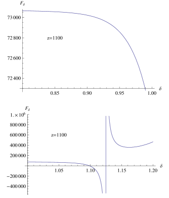
Figure 1: In this plot is represented $F_{\delta}$ vs $\delta$ for $\delta\leq 1$ (upper plot) and $\delta\geq 1$ (lower plot). The condition that the eccentricity is positive follows for $F_{\delta}>0$.

4 Light propagation in NLED and birefringence

In this Section we discuss the modification of the light velocity (birefringence effect) for the model of nonlinear electrodynamics $L(X,Y)$. We shall follow the paper [34] (see also [2, 35]), in which is studied the propagation of wave in local nonlinear electrodynamics by making use of the Fresnel equation for the wave covectors $k_{\mu}$. The latter are related to phase velocity $v$ of the wave propagation by the relation $k_{i}=\displaystyle{\frac{k_{0}}{v}{\hat{k}}_{i}}$, where ${\hat{k}}_{i}$ are the components of the unit 3-covector. Thus, in what follows we confine ourselves to the phase velocity. It is straightforward to show that for the models under consideration (4) the group velocity is always greater or equal to the phase velocity [34].

The main result in Ref. [34] corresponds to the optic metric tensors

$$g_{1}^{\mu\nu}={\cal X}g^{\mu\nu}+({\cal Y}+\sqrt{{\cal Y}-{\cal X}{\cal Z}})t^{\mu\nu}\,,$$ (39)

$$g_{2}^{\mu\nu}={\cal X}g^{\mu\nu}+({\cal Y}-\sqrt{{\cal Y}-{\cal X}{\cal Z}})t^{\mu\nu}\,,$$ (40)

which describe the effect of birefringent light propagation in a generic model for nonlinear electrodynamics. The quantities ${\cal X}$, ${\cal Y}$, and ${\cal Z}$ are related to the derivatives of the Lagrangian $L(X,Y)$ with respect to the invariant $X$ and $Y$, and $t^{\mu\nu}=F^{\mu\alpha}F^{\nu}_{\,\,\alpha}$.

For our model, expressed byEq. (4), the quantities ${\cal X}$, ${\cal Y}$, and ${\cal Z}$ are given by

$${\cal X}\equiv K_{1}^{2}=\frac{\gamma^{2}\delta^{2}}{4}X^{2(\delta-1)}\,,\quad{\cal Y}\equiv K_{1}K_{2}=\frac{\gamma^{2}\delta^{2}}{4}\,(\delta-1)X^{2(\delta-1)-1}\,,\quad{\cal Z}=0\,,$$

where $K_{1}=\displaystyle{4\frac{\partial L}{\partial X}}$ and $K_{2}=8\displaystyle{\frac{\partial^{2}L}{\partial X^{2}}}$, while the metrics (39) and (40) are

$$g^{\mu\nu}_{1}=K_{1}(K_{1}g^{\mu\nu}+2K_{2}t^{\mu\nu})\,,\quad g^{\mu\nu}_{2}=K_{1}^{2}g^{\mu\nu}.$$

As a consequence, birefringence is present in our model. This means that some photons propagate along the standard null rays of spacetime metric $g^{\mu\nu}$, whereas other photons propagate along rays null with respect to the optical metric $K_{1}g^{\mu\nu}+2K_{2}t^{\mu\nu}$.

The velocities of the light wave can be derived by using the light cone equations (effective metric)

$$g_{1}^{\mu\nu}k_{\mu}k_{\nu}=0\quad{\rm and}\quad g_{2}^{\mu\nu}k_{\mu}k_{\nu}=0\,.$$

It is worthwhile to report the general expression for the average value of the velocity scalar [34]

$$\langle v^{2}\rangle=1+\frac{4}{3}\frac{T^{00}({\cal Y}+{\cal Z}t^{00})}{{\cal X}+2{\cal Y}t^{00}+{\cal Z}(t^{00})^{2}}+\frac{2}{3}{\bf S}^{2}\,\frac{2{\cal Y}^{2}-{\cal X}{\cal Z}+{\cal Z}(t^{00})^{2}+2{\cal Y}{\cal Z}t^{00}}{[{\cal X}+2{\cal Y}t^{00}+{\cal Z}(t^{00})^{2}]^{2}}$$

where $T^{00}=-t^{00}+X=({\bf E}_{\gamma}^{2}+{\bf B}_{\gamma}^{2})/2$ ($t^{00}=-{\bf E}_{\gamma}^{2}$), and ${\bf S}^{2}=\delta_{\mu\nu}t^{0\mu}t^{0\nu}$, where ${\bf S}={\bf E}\times{\bf B}$ is the energy flux density. The subscript $\gamma$ is introduced for distinguishing the photon field from the magnetic background. The value of the mean velocity has been derived averaging over the directions of propagation and polarization. For our model, we get

$$\langle v^{2}\rangle\simeq 1+(\delta-1)R+(\delta-1)^{2}S\,,$$ (41)

$$R\equiv\frac{4}{3}\frac{T^{00}}{4X+2(\delta-1)t^{00}}\,,\quad S=\frac{4}{3}\frac{{\bf S}^{2}}{[4X+2(\delta-1)t^{00}]^{2}}$$

The high accuracy of optical experiments in laboratories requires tiny deviations from standard electrodynamics. This condition is satisfied provided $|\delta-1|\ll 1$. Moreover, there are two aspects related to (41):

• The average velocity does depend on (only) the parameter $\delta$, so that $\gamma$ or $\Lambda$ in our model can be fixed independently. This task is addressed in the next Section.

• Because $R$ is positive, one has to demand that $\delta-1<0$ in order that $v^{2}<1$.

The above considerations hold for flat spacetime, and can be straightforwardly generalized to the case of curved space time [34].

5 Stokes parameters, rotated CMB spectra and constraints on parameter $\Lambda$

The propagation of photons can be described in terms of the Stokes parameters $I$, $Q$, $U$, and $V$. The parameters $Q$ and $V$ can be decomposed in gradient-like ($G$) and a curl-like ($C$) components [32] ($G$ and $C$ are also indicated in literature as $E$ and $B$), and characterize the orthogonal modes of the linear polarization (they depend on the axes where the linear polarization are defined, contrarily to the physical observable $I$ and $V$ which are independent on the choice of coordinate system).

The polarization $G$ and $C$ and the temperature ($T$) are crucial because they allow to completely characterize the CMB on the sky. If the Universe is isotropic and homogeneous and the electrodynamics is the standard one, then the $TC$ and $GC$ cross-correlations power spectrum vanish owing to the absence of the cosmological birefringence. In presence of the latter, on the contrary, the polarization vector of each photons turns out to be rotated by the angle $\Delta\alpha$, giving rise to $TC$ and $GC$ correlations.

Using the expression for the power spectra $C_{l}^{XY}\sim\int dk[k^{2}\Delta_{X}(t_{0})\Delta_{Y}(t_{0})]$, where $X,Y=T,G,C$ and $\Delta_{X}$ are the polarization perturbations whose time evolution is controlled by the Boltzman equation, one can derive the correlation for $T$, $G$ and $C$ in terms of $\Delta\alpha$ [14]

$$C_{l}^{\prime\,TC}=C_{l}^{TC}\sin 2\Delta\alpha\,,\quad C_{l}^{\prime\,TG}=C_{l}^{TG}\cos 2\Delta\alpha\,,$$ (42)

$$C_{l}^{\prime\,GC}=\frac{1}{2}\left(C_{l}^{GG}-C_{l}^{CC}\right)\sin 4\Delta\alpha\,,$$ (43)

$$C_{l}^{\prime\,GG}=C_{l}^{GG}\cos^{2}2\Delta\alpha+C_{l}^{CC}\sin^{2}2\Delta\alpha\,,$$ (44)

$$C_{l}^{\prime\,CC}=C_{l}^{CC}\cos^{2}2\Delta\alpha+C_{l}^{GG}\sin^{2}2\Delta\alpha\,.$$ (45)

The prime indicates the rotated quantities. Notice that the CMB temperature power spectrum remains unchanged under the rotation.

Experimental constraints on $\Delta\alpha$ have been put from the observation of CMB polarization by WMAP and BOOMERanG [14, 27].

$$\Delta\alpha=(-2.4\pm 1.9)^{\circ}=[-0.0027\pi,-0.0238\pi]\,.$$ (46)

The combination of Eqs. (46) and (35), and the laboratory constraints $|\delta-1|\ll 1$ allow to estimate $\Lambda$.

5.1 Estimative of $\Lambda$

To estimate $\Lambda$ we shall write

$$B = 10^{-9+b}\,{\rm G}\qquad\,\,\,b\lesssim 2\,,$$ (47)

$$F_{\delta} = 2z^{3/2}\qquad\qquad z=1100\gg 1\,.$$ (48)

The bound (46) can be therefore rewritten in the form

$$\frac{10^{-3}}{\cal A}\lesssim|\delta-1|\lesssim\frac{10^{-2}}{\cal A}\,,$$ (49)

where

$${\cal A}\equiv\frac{9K}{14}\,F_{\delta}\Omega_{B}^{(0)}\simeq K\,10^{-6+2b}\left[0.24\times 10^{-56+2b}\left(\frac{\rm GeV}{\Lambda}\right)^{4}\right]^{\delta-1}\,.$$ (50)

The condition $|\delta-1|\ll 1$ requires ${\cal A}\gg 1$. It turns out convenient to set

$${\cal A}=10^{a}\,,\qquad a>{\cal O}(1)\,.$$ (51)

From Eqs. (50) and (51) it then follows

$$\Lambda=10^{-14+b/2}\left[\frac{1}{K}\,10^{a-2b+6}\right]^{-\frac{1}{4(\delta-1)}}\rm GeV\,,$$ (52)

or equivalently

$${\rm Log}\left[\frac{\Lambda}{\rm GeV}\right]=\left(-14+\frac{b}{2}\right)+\frac{(-1)}{4(\delta-1)}\left[a-2b+6-{\rm Log}K\right]\,.$$ (53)

The constant $K$ can now be determined to fix the characteristic scale $\Lambda$. Writing $\Lambda=10^{\Lambda_{x}}$ GeV, where $\Lambda_{x=Pl}=19$, $\Lambda_{\rm GUT}=16$ and $\Lambda_{\rm EW}=3$ for the Planck, GUT and electroweak (EW) scales, respectively, Eq. (53) yields

$$K=10^{a-2b+6-\zeta}\,,\qquad\zeta\equiv\frac{4(\delta-1)\Lambda_{x}}{14-b/2}\ll 1\,.$$ (54)

In Fig. 2 is plotted Log$(\Lambda$/GeV) vs $K$ for fixed values of the parameters $a$, $b$ and $\delta-1$. Similar plots can be derived for GUT and EW scales

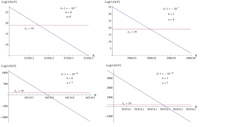
Figure 2: $\Lambda$ vs $K$ for different values of the parameter $\delta-1$, $a$ and $b$. The parameter $a$ is related to the range in which $\delta-1$ varies, i.e. $-10^{-3-a}\lesssim\delta-1\lesssim-10^{-2-a}$, while $b$ parameterizes the magnetic field strength $B=10^{-9+b}$ G. The red-shift is $z=1100$. Plot refers to Planck scale $\Lambda=10^{\Lambda_{x}}$ GeV, with $\Lambda_{x=Pl}=19$. Similar plots can be also obtained for GUT ($\Lambda_{\rm GUT}=16$) and EW ($\Lambda_{\rm EW}=3$) scales.

6 Discussion and closing remarks

In conclusion, in this paper we have calculated, in the framework of the nonlinear electrodynamics, the rotation of the polarization angle of photons propagating in a Universe with planar symmetry. We have found that the rotation of the polarization angle does depend on the parameter $\delta$, which characterizes the degree of nonlinearity of the electrodynamics. This parameter can be constrained by making use of recent data from WMAP and BOOMERang. Results show that the CMB polarization signature, if detected by future CMB observations, would be an important test in favor of models going beyond the standard model, including the nonlinear electrodynamics.

Some comments are in order. In our investigation we have assumed that the planar-symmetry is induced by a magnetic field. This is not the unique case. In fact, a planar geometry can also be induced by topological defects, such as cosmic string ($cs$) or domain wall ($dw$) [21]. In such a case, one has [21]

$$e^{2}\Biggl{|}_{dw}=\frac{2}{7}\Omega_{dw}^{(0)}\left[\frac{3}{(1+z)^{2}}+4(1+z)^{3/2}-7\right]\,,$$ (55)

and

$$e^{2}\Biggl{|}_{cs}=\frac{4}{5}\Omega_{cs}^{(0)}\left[\frac{3}{(1+z)}+2(1+z)^{3/2}-5\right]\,,$$ (56)

where $\Omega_{(dw,cs)}^{(0)}$ are the present energy densities, in units of critical density, of the domain wall and cosmic string. At the decoupling, one obtains

$$e^{2}(z_{dec})\Biggl{|}_{dw}\simeq 10^{-4}\frac{\Omega_{dw}^{(0)}}{5\times 10^{-7}}\,,$$ (57)

and

$$e^{2}(z_{dec})\Biggl{|}_{cs}\simeq 10^{-4}\frac{\Omega_{cs}^{(0)}}{4\times 10^{-7}}\,.$$ (58)

The analysis leading to determine the bounds on $\delta$ from CMB polarization goes along the line above traced.

Moreover, a complete analysis of the planar-geometry is required to fix the parameter $\delta$. From a side, in our calculations in fact we have assumed that the Universe is matter dominated. A more precise calculation should require to use (to solve (31)) the relation

$$t=\displaystyle{\frac{1}{H_{0}}\int_{0}^{z}\frac{1+z}{\sqrt{\Omega_{m}(1+z)^{3}+\Omega_{\Lambda}}}\,dz}\;,$$ (59)

where $\Omega_{m}=0.3$, $\Omega_{\Lambda}=0.7$ and $H_{0}=72$ km sec^-1 Mpc^-1 ($z=1100$). From the other side, a complete study of the Eq. (31) is necessary in order to put stringent constraints on the parameter $\delta$.

As closing remark, we would like to point out that the approach to analyze the CMB polarization in the context of NLED that we have presented above can also be applied to discuss the extreme-scale alignments of quasar polarization vectors [38], a cosmic phenomenon that was discovered by Hutsemekers[36] in the late 1990’s, who presented paramount evidence for very large-scale coherent orientations of quasar polarization vectors (see also Hutsemekers and Lamy [37]).. As far as the authors of the present paper are awared of, the issue has remained as an open cosmological connundrum, with a few workers in the field having focused their attention on to those intriguing observations. Nonetheless, we quote “en passant” that in a recent paper [39] Hutsemekers et al. discussed the possibility of such phenomenon to be understood by invoking very light pseudoscalar particles mixing with photons. They claimed that the observations of a sample of 355 quasars with significant optical polarization present strong evidence that quasar polarization vectors are not randomly oriented over the sky, as naturally expected. Those authors suggest that the phenomenon can be understood in terms of a cosmological-size effect, where the dichroism and birefringence predicted by a mixing between photons and very light pseudoscalar particles within a background magnetic field can qualitatively reproduce the observations. They also point out at a finding indicating that circular polarization measurements could help constrain their mechanism.

Since cosmic magnetic fields have a typical strength of $\sim 10^{-7}-10^{-8}$ G, on average, for a characteristic distance scale of 10-30 Mpc, it is our view that such phenomenology can be understood in the framework of a nonlinear description of photon propagation (NLED) over cosmic background magnetic fields and the use of a planar symmetry for the space-time. Specifically, phenomena involving light propagation as dichroism and birefringence can be inscribed on to the framework of Heisenberg-Euler NLED, which predicts the occurrence of birefringence on cosmological distance scales. We plan to present such analysis in a forthcoming communication [40].

Acknowledgments: The authors express their gratitude to the referee for relevant comments. The authors also thank Prof. Xin-min Zhang, and Dr. Mingzhe Li for reading the manuscript and their suggestions. H.J.M.C. thanks ICRANet International Coordinating Center, Pescara, Italy for hospitality during the early stages of this work. G.L. acknowledges the financial support of MIUR through PRIN 2006 Prot. $1006023491_{-}003$, and of research funds provided by the University of Salerno.

References

References

- [1] M. Born, Nature (London) 132, 282 (1933); Proc. R. Soc. A 143, 410 (1934). M. Born, L. Infeld, Nature (London) 132, 970 (1933); Proc. R. Soc. A 144, 425 (1934). W. Heisenberg, H. Euler, Z. Phys. 98, 714 (1936). J. Schwinger, Phys. Rev. 82, 664 (1951).
- [2] S.A. Guiterrez, A.L. Dudley, and J.F. Plebanski, J. Math. Phys. 22, 2835 (1981). J.F. Plebanski, Lectures on nonlinear electrodynamics, monograph of the Niels Bohr Institute (Nordita, Copenhagen, 1968).
- [3] P. Moniz, Phys. Rev. D 66, 103501 (2002). R. Garcia-Salcedo, N. Breton, Int. J. Mod. Phys. A15, 4341 (2000); Class. Quant. Grav. 20. 5425 (2003); Class. Quant. Grav. 22, 4783 (2005). V.V. Dyadichev, D.V. Galt’tsov, A.G. Zorin, and M. Yu. Zotov, Phys. Rev. D 65, 084007 (2002). D.V. Vollick, Gen. Rel. Grav. 35, 1511 (2003). L. Hollenstein, F.S.N. Lobo, arXiv:0807.2325 [gr-qc]. H.J. Mosquera Cuesta, J.M. Salim, M. Novello, arXiv:0710.5188 [astro-ph]. K. Bamba, S. Nojiri, arXiv:0811.0150 [hep-th]. K. Bamba, S.D. Odintsov, JCAP04 (2008) 024.
- [4] E. Ayon-Beato, A. Garcia, Phys. Rev. Lett. 80, 5056 (1998); Phys. Lett. B 464, 25 (1999); Gen. Rel. Grav. 31, 629 (1999). N. Breton, Phys. Rev. D 72, 044015 (2005). K.A. Bronnikov, Phys. Rev. D 63, 044005 (2001). A. Burinskii, S.R. Hildebrandt, Phys. Rev. D 65, 104017 (2002). M. Cataldo, A. Garcia, Phys. Rev. D 61, 084003 (2000).
- [5] A.V.B Arellano, F.S.N. Lobo, Class. Quant. Grav, 23, 5811 (2006); gr-qc/0604095. K.A. Bronnikov, S.V. Grinyok, Grav. Cosmol. 11, 75 (2006). F. Baldovin, M. Novello, S.E Pérez Bergliaffa, J.M. Salim, Class. Quant. Grav. 17, 3265 (2000).
- [6] Mingzhe Li, Jun-Qing Xia, Hong Li, and Xinmin Zhang, Phys. Lett. B 651, 357 (2007)
- [7] See the derivation of the rotation angle formulas in a fully general relativistic approach by Mingzhe Li, Xinmin Zhang, Phys. Rev. D 78, 103516 (2008). e-print: arXiv:0810.0403v2 [astro-ph].
- [8] H.J. Mosquera Cuesta, G. Lambiase, Phys. Rev. D 80, 023013 (2009).
- [9] K.E. Kunze, Phys. Rev. D 77, 023530 (2008).
- [10] J.D. Barrow, R. Marteens, Ch.G. Tsagas, Phys. rep. 449, 131 (2007).
- [11] L. Campanelli, P. Cea, G.L. Fogli, L. Tedesco, Phys. Rev. D 77, 043001 (2008); Phys. Rev. D 77, 123002 (2008).
- [12] A.K. Harding, M.G. Baring, and P.L. Gonthier, Astrophys. J. 476, 246 (1997). M.G. Baring, A.K. Harding, Astrophys. J. Lett. 507, L55 (1998). M.G. Baring, Phys. Rev. D 62, 016003 (2000). A.K. Harding and D. Lai, Rep. Prog. Phys. 69, 2631 (2006). H. J. Mosquera Cuesta and J. M. Salim, MNRAS 354, L55 (2004). H. J. Mosquera Cuesta and J. M. Salim, ApJ 608, 925 (2004). H. J. Mosquera Cuesta, J. A. de Freitas Pacheco and J. M. Salim, IJMPA 21, 43 (2006) J-P. Mbelek, H. J. Mosquera Cuesta, M. Novello and J. M. Salim Eur. Phys. Lett. 77, 19001 (2007).
- [13] J-Q Xia, H. Li, X. Zhang, arXiv:0908.1876v2 [astro-ph.CO]. See also B. Feng, M. Li, J. Q. Xia, X. Chen, and X. Zhang, Phys. Rev. Lett. 96, 221302 (2006).
- [14] G. Gubitosi, L. Pagano, G. Amelino-Camelia, A. Melchiorri, A. Cooray, JCAP 0908:021 (2009). M. Das, S. Mohanty, A.R. Prasanna, arXiv:0908.0629v1 [astro-ph.CO]. P. Cabella, P. Natoli, J. Silk, Phys. Rev. D 76, 123014 (2007). F.R. Urban, A.R. Zhitnitsky, arXiv:1011.2425 [astro-ph.CO]. G.-C. Liu, S. Lee, K.-W. Ng, Phys. Rev. Lett. 97, 161303 (2006). Y.-Z. Chu, D.M.Jacobs, Y. Ng, D. Starkman, Phys. Rev. D 82, 064022 (2010). S. di Serego Alighieri, arXiv:1011.4865 [astro-ph.CO].
- [15] R. Sung, P. Coles, arXiv:1004.0957v1[astro-ph.CO].
- [16] H. Pagels, E. Tomboulis, Nucl. Phys. B 143, 485 (1978). H. Arodz, M. Slusarczyk, A. Wereszcynski, Acta. Pol. B 32, 2155 (2001). M. Slusarczyk, A. Wereszcynski, Acta. Pol. B 34, 2623 (2003).
- [17] J. P. Mbelek, H. J. Mosquera Cuesta, MNRAS 389, 199 (2008).
- [18] M. Novello, S.E. Pérez Bergliaffa, J. Salim, Phys. Rev. D 69, 127301 (2004).
- [19] C.W. Misner, K.S. Thorne, J.A. Wheeler, Gravitation, Freeman Press, San Francisco, 1973.
- [20] A.H. Taub, Ann. Math. 53, 472 (1951).
- [21] L. Campanelli, P. Cea, L. Tedesco, Phys. Rev. D 76, 063007 (2007); Phys. Rev. Lett. 97, 131302 (2006).
- [22] Notice that the cases discussed in [21], i.e. the magnetic fields or the topological defects as responsible of the planar symmetry of the Universe, allow to explain the anomaly concerning the low quadruple amplitude probed by WMAP. The interesting analysis performed by CCT leads to the conclusion that an eccentricity at the decoupling of the order of is indeed able to explain the drastic reduction in the quadruple anisotropy without affecting higher multiples of the angular power spectrum of the temperature anisotropies.
- [23] E.N. Parker, Cosmological Magnetic Fields (Oxford University Press, Oxford, England, 1979). Ya. B. Zeldovich, A.A. Ruzmaikin, D.D. Sokoloff, Magnetic Fields in Astrophysics (Gordon & Breach, NY, 1980).
- [24] M. Giovannini, Int. J. Mod. Phys. D 13, 391 (2004). L.M. Widrow, Rev. Mod. Phys. 74, 775 (2002). D. Grasso, H.R. Rubinstein, Phys. Rep. 348, 163 (2001). P.P. Kronberg, Rep. Prog. Phys. 57, 325 (1994). A.D. Dolgov, hep-ph/0110293. J.-P. Valleé, New Astron. Rev. 48, 763 (2004).
- [25] M.S. Turner, L.M. Widrow, Phys. Rev. D 37, 2743 (1988). See also L. Campanelli, P. Cea, G.L. Fogli, L. Tedesco, Phys. Rev. D 77, 043001 (2008); Phys. Rev. D 77, 123002 (2008). T. Vachaspati, Phys. Lett. B 265, 258 (1991). B. Cheng, A. Olinto, Phys. Rev. D bf 50, 2421 (1994). A.P. Martin, A.C. Davies, Phys. Lett. B 360, 71 (1995). T.W.B. Kibble, A. Vilenkin, Phys. Rev. D 52, 679 (1995). M. Gasperini, M. Giovannini, G. Veneziano, Phys. Rev. Lett. 75, 3796 (1995). M. Gasperini, Phys. Rev. D 63, 047301 (2001). M. Giovannini, M. Shaposhnikov, Phys. Rev. D 62, 103512 (2000). G.B. Field, S.M. Carroll. Phys. Rev. D 62, 103008 (2000). B. Ratra, Astrophys. J. Lett. 391, L1 (1992). E. Calzetta, A. Kandus, F. Mazzitelli, Phys. Rev. D 57, 7139 (1998). G. Lambiase, A.R. Prasanna, Phys. Rev. D 70, 063502 (2004). G. Lambiase, S. Mohanty, G. Scarpetta, JCAP 07 (2008) 019. R. Opher, U.F. Wichoski, Phys. Rev. Lett. 78, 787 (1997). K. Bamba, JCAP 0710 015 (2007); Phys.Rev.D 75, 083516 (2007).K. Bamba, C.Q. Geng, S.H. Ho, astro-ph/0806.1856. F.D. Mazzitelli, F.M. Spedalieri, Phys. Rev. D 52, 6694 (1995). W.D. Garretson, G.B. Field, S.M. Carroll, Phys. Rev. D 46, 5346 (1992). S.M. Carroll, G.B. Field, R. Jackiw, Phys. Rev. D 41, 1231 (1990). D. Harari, P. Sikivie, Phys. Lett. B 289, 67 (1992). S. Matarrese, S. Mollerach, A. Notari, A. Riotto, Phys. Rev. D 71, 043502 (2005). A.L. Maroto, Phys. Rev. D 64, 083006 (2001). E. Fenu and R. Durrer, astr-ph/0809.1383. C.G. Tsagas, P.K.S. Dunsby, and M. Maklund, Phys. Lett. B 561, 17 (2003). C.G. Tsagas, Phys. Rev. D 72, 123509 (2005). A.D. Dolgov, D. Grasso, Phys. Rev. Lett. 88, 011301 (2001). J.D. Barrow, C.G. Tsagas, Phys. Rev. D 77, 107302 (2008). O. Bertolami, D.F. Mota, Phys. Lett. B 455, 96 (1999). T. Vachaspati, A. Vilenkin. Phys. Rev. Lett. 67, 1057 (1991). M. Joyce, M. Shaposhnikov, Phys. Rev. Lett, 79, 1193 (1997). A. Dolgov, J. Silk, Phys. Rev. D 47, 3144 (1993). A. Dolgov, Phys. Rev. D 48, 2499 (1993). V.B. Semikoz, D.D. Sokoloff, Phys. Rev. Lett. 92, 131301 (2004). J.H. Piddington, Aust. J. Phys. 23, 731 (1970). L.M. Widrow, Rev. Mod. Phys. 74, 775 (2002). D. Grasso, H.R. Rubinstein, Phys. Rep. 348, 163 (2001). K. Enqvist, Int. J. Mod. Phys. D 7, 331 (1998). S. Koh, C.H. Lee, Phys. Rev. D 62, 083509 (2000). J. Barrow, P. Ferreira, J. Silk, Phys. Rev. Lett. 78, 3610 (1997). J. Barrow, Phys. Rev. D 55, 7451 (1997). A. Kosowsky, A. Loeb, ApJ 461, 1 (1996). M. Giovannini, Phys. Rev. D 56, 3198 (1997). T. Kolatt, astro-ph/9704243. D. Grasso, H. Rubinstein, Astropart. Phys. 3, 4714 (1995); Phys. Lett B 379, 73 (1996). P. Kernan, G. Starkman, T. Vachaspati, Phys. Rev. D 54, 7207 (1996). B. Cheng, A. Olinto, D.N. Schramm, J. Truran, Phys. Rev. D 54, 4714 (1996). B. Cheng, D.N. Schramm, J. Truran, Phys. Rev. D 49, 5006 (1994). G. Greenstein, Nature 223, 938 (1968).
- [26] H.R. Rubinstein, Int. J. of Theor. Phys. 38, 1315 (1999).
- [27] J.Q. Xia, H. Li, G.B. Zhao, X. Zhang, Astrophys. J. 679, L61 (2008).
- [28] E.W. Kolb, M.S. Turner, The Early Universe (addison-Wesley, Reading, MA, 1990).
- [29] D. Grasso, H.R. Rubinstein, Phys. Lett. B 379, 73 (1996).
- [30] W. Hu, U. Seljak, M. White, M. Zaldarriaga, Phys. Rev. D 57, 3290 (1998).
- [31] A. Lue, L.M. Wang, M. Kamionkowski, Phys. Rev. Lett. 83, 1506 (1999).
- [32] M. Kamionkowski, A. Kosowski, A. Stebbins, Phys. Rev. D 55, 7368 (1997).
- [33] B. Feng, H. Li, X. Zhang, Phys. Lett. B 620, 27 (2005).
- [34] Y.N. Obukhov, G.F. Rubilar, Phys. Rev. D 66, 024042 (2002).
- [35] M. Novello, V.A. De Lorenci, J.M. Salin, R. Klippert, Phys. Rev. D 61, 045001 (2000). M. Novello, S.E. Pérez Bergliaffa, J. Salim, Phys. Rev. D 69, 127301 (2004). V.A. De Lorenci, R. Klippert, M. Novello, J.M. Salim, Phys. Lett. B 482, 134 (2000). V.A. De Lorenci, M.A. Souza, Phys. Lett. B 512, 417 (2001). V.A. De Lorenci, R. Klippert, Phys. Rev. D 65, 064027 (2002). G.W. Gibbons, C.A.R. Herdeiro, Phys. Rev. D 65, 064006 (2001). J.P.S. Lemos, R. KErner, Grav. Cosmol. 6, 49 (2000). I.T. Drummond, S.J. Hathrell, Phys. Rev. D 22, 343 (1980). J.I. Latorre, P. Pascual, R. Tarrach, Nucl. Phys. B 437, 60 (1995). G.M. Shore, Nucl. Phys. B 460, 379 (1996). W. Dittrich, H. Gies, Phys. Rev. D 58, 025004 (1998). H. Gies, Phys. Rev. D 60, 105033 (1999). D.I. Blokhintsev, V.V. Orlov, Zh. Eksp. Fiz. 25, 513 (1953). M. Lutzky, J.S. Toll, Phys. Rev. 113, 1649 (1959). H.S. Ibarguen, A. Garcia, J. Plebanski, J. Math. Phys. 30, 2689 (1989). S.L. Adler, Ann. Phys. (N.Y.) 67, 599 (1971). Z. Bialynicka-Birula, I. Bialynicki-Birula, Phys. Rev. D 2, 2341 (1970). W.-Y. Tsai, T. Erber, Phys. Rev. D 12, 1132 (1975).
- [36] D. Hutsemekers, Astron. Astrophys 332, 410 (1998)
- [37] D. Hutsemekers, H. Lamy, Astron. Astrophys 358, 835 (2000)
- [38] D. Hutsemekers, R. Cabanac, H. Lamy, D. Sluse, Astron.Astrophys. 441, 915-930 (2005)
- [39] D. Hutsemekers, A. Payez, R. Cabanac, H. Lamy, D. Sluse, B. Borguet, J.-R. Cudell, Large-Scale Alignments of Quasar Polarization Vectors: Evidence at Cosmological Scales for Very Light Pseudoscalar Particles Mixing with Photons? . (2008). e-Print: arXiv:0809.3088 [astro-ph]
- [40] H. J. Mosquera Cuesta, G. Lambiase, in preparation (2011)