A Gaussian mixture ensemble transform filter

Abstract

We generalize the popular ensemble Kalman filter to an ensemble transform filter where the prior distribution can take the form of a Gaussian mixture or a Gaussian kernel density estimator. The design of the filter is based on a continuous formulation of the Bayesian filter analysis step. We call the new filter algorithm the ensemble Gaussian mixture filter (EGMF). The EGMF is implemented for three simple test problems (Brownian dynamics in one dimension, Langevin dynamics in two dimensions, and the three dimensional Lorenz-63 model). It is demonstrated that the EGMF is capable to track systems with non-Gaussian uni- and multimodal ensemble distributions.

1 Introduction

We consider dynamical models given in the form of ordinary differential equations (ODEs)

$$\dot{\bf x}=f({\bf x},t)$$ (1)

with state variable ${\bf x}\in\mathbb{R}^{N}$. Initial conditions at time $t_{0}$ are not precisely known and are treated as a random variable instead, i.e., we assume that

$${\bf x}(t_{0})\sim\pi_{0},$$

where $\pi_{0}({\bf x})$ denotes a given probability density function (PDF). The solution of (1) at time $t$ with initial condition ${\bf x}_{0}$ at $t_{0}$ is denoted by ${\bf x}(t;t_{0},{\bf x}_{0})$.

The evolution of the initial PDF $\pi_{0}$ under the ODE (1) up to a time $t>t_{0}$ is provided by the continuity equation

$$\frac{\partial\pi}{\partial t}=-\nabla_{\bf x}\cdot(\pi f),$$ (2)

which is also called Liouville’s equation in the statistical mechanics literature (Gardiner, 2004). Let us denote the solution of Liouville’s equation at observation time $t$ by $\pi({\bf x},t)$. In other words, solutions ${\bf x}(t;t_{0},{\bf x}_{0})$ with ${\bf x}_{0}\sim\pi_{0}$ constitute a random variable with PDF $\pi(\cdot,t)$.

For a chaotic ODE (1), i.e. for an ODE with positive Lyapunov exponents, the PDF $\pi(\cdot,t)$ will be spread out over the whole chaotic attractor for $t\to\infty$. This in turn implies a limited solution predictability in the sense that the time-evolved PDF will become increasingly independent of the initial PDF $\pi_{0}$. Furthermore, even if the initial PDF is nearly Gaussian with mean $\overline{\bf x}_{0}$ and small covariance matrix ${\bf P}$, the solution ${\bf x}(t;t_{0},\overline{\bf x}_{0})$ will become increasingly unrepresentative of the expectation value of the underlying random variable it is supposed to represent.

To counteract the divergence of nearby trajectories under chaotic dynamics, we assume that we have uncorrelated measurements ${\bf y}_{\rm obs}(t_{j})\in\mathbb{R}^{K}$ at times $t_{j}$, $j\geq 1$ with measurement error covariance matrix ${\bf R}\in\mathbb{R}^{K\times K}$, i.e.

$${\bf y}_{\rm obs}(t_{j})-{\bf H}{\bf x}(t_{j})\sim{\rm N}({\bf 0},{\bf R}),$$ (3)

where the notation ${\rm N}(\overline{\bf y},{\bf B})$ is used to denote a normal distribution in ${\bf y}\in\mathbb{R}^{K}$ with mean $\overline{\bf y}$ and covariance matrix ${\bf B}\in\mathbb{R}^{K\times K}$. The matrix ${\bf H}\in\mathbb{R}^{K\times N}$ is called the forward operator. The task of combining solutions to (1) with intermittent measurements (3) is called data assimilation in the geophysical literature (Evensen, 2006) and filtering in the statistical literature (Bain and Crisan, 2009).

A first step to perform data assimilation for nonlinear ODEs (1) is to approximate solutions to the associated Liouville equation (2). In this paper, we rely exclusively on particle methods (Bain and Crisan, 2009) for which Liouville’s equation is naturally approximated by the evolving empirical measure. More precisely, particle or ensemble filters rely on the simultaneous propagation of $M$ independent solutions ${\bf x}_{i}(t)\in\mathbb{R}^{N}$, $i=1,\ldots,M$, of (1) (Evensen, 2006). We associate the empirical measure

$$\pi_{\rm em}({\bf x},t)=\sum_{i=1}^{M}\gamma_{i}\delta({\bf x}-{\bf x}_{i}(t))$$ (4)

with weights $\gamma_{i}>0$ satisfying

$$\sum_{i=1}^{M}\gamma_{i}=1.$$

Here $\delta(\cdot)$ denotes the Dirac delta function. Hence our statistical model is given by the empirical measure (4) and is parametrized by the particle weights $\{\gamma_{i}\}$ and the particle locations $\{{\bf x}_{i}\}$. In the absence of measurements, the empirical measure $\pi_{\rm em}$ with constant weights $\gamma_{i}$ is an exact (weak) solution to Liouville’s equation (2) provided the ${\bf x}_{i}(t)$’s are solutions to the ODE (1). Optimal statistical efficiency is achieved with equal particle weights $\gamma_{i}=1/M$.

The assimilation of a measurement at $t_{j}$ leads via Bayes’ theorem to a discontinuous change in the statistical model (4). Sequential Monte Carlo methods (Bain and Crisan, 2009) are primarily based on a discontinuous change in the weight factors $\gamma_{i}$. To avoid a subsequent degeneracy in the particle weights one re-samples or uses other techniques which essentially lead to a redistribution of particle positions ${\bf x}_{i}$. See, for example, Bain and Crisan (2009) for more details. The ensemble Kalman filter (EnKF) relies on the alternative idea to replace the empirical measure (4) by a Gaussian PDF prior to an assimilation step (Evensen, 2006). This approach allows for the application of the Kalman analysis formulas to the ensemble mean and covariance matrix. The final step of an EnKF is the re-interpretation of the Kalman analysis step in terms of modified particle positions while the weights are held constant at $\gamma_{i}=1/M$. We call filter algorithms that rely on modified particle/ensemble positions and fixed particle weights ensemble transform filters. A new ensemble transform filter has recently been proposed by Anderson (2010). The filter is based on an appropriate transformation step in observation space and subsequent linear regression of the transformation onto the full state space. The approach developed in this paper relies instead on a general methodology for deriving ensemble transform filters as proposed by Reich (2011). See Section 2 below for a summary. The same methodology has been developed for continuous-in-time observations by Crisan and Xiong (2010). In this paper, we demonstrate how our ensemble transform filter framework can be used to generalize EnKFs to Gaussian mixture models and Gaussian kernel density estimators. The essential steps are summarized in Section 3 while an algorithmic summary of the proposed ensemble Gaussian mixture filter (EGMF) is provided in Section 4. The EGMF can also be viewed as a generalization of the continuous formulation of ensemble square root filters (Tippett et al., 2003) as provided by Bergemann and Reich (2010a, b) and the EnKF with perturbed observations, as demonstrated by Reich (2011). The paper concludes with three numerical examples in Section 5. We first demonstrate the properties of the newly proposed EGMF for one-dimensional Brownian dynamics under a double-well potential. This simulation is extended to the associated two-dimensional Langevin dynamics model with only velocities being observed. Finally we consider the three variable model of Lorenz (1963).

We mention that alternative extensions of the EnKF to Gaussian mixtures have recently been proposed, for example, by Smith (2007), Stordal et al. (2011), and Frei and Künsch (2011). However, while the cluster EnKF of Smith (2007) is an example of an ensemble transform filter, it fits the posterior (analysed) ensemble distribution back to a single Gaussian PDF and, hence, only partially works with a Gaussian mixture. Both the mixture ensemble Kalman filter of Frei and Künsch (2011) and the adaptive Gaussian mixture filter of Stordal et al. (2011) approximate the model uncertainty by a sum of Gaussian kernels and utilize the ensemble Kalman filter as a particle update step under a single Gaussian kernel. Resampling or a re-weighting of particles is required to avoid a degeneracy of particle weights due to changing kernel weights. A related filter algorithm based on Gaussian kernel density estimators has previously been considered by Anderson and Anderson (1999).

2 A general framework for ensemble transform filters

Bayes’ formula can be interpreted as a discontinuous change of a forecast PDF $\pi_{f}$ into an analyzed PDF $\pi_{a}$ at each observation time $t_{j}$. On the other hand, one can find a continuous embedding $\pi({\bf x},s)$ with respect to a fictitious time $s\in[0,1]$ such that $\pi(\cdot,0)=\pi_{f}$ and $\pi_{a}=\pi(\cdot,1)$. As proposed by Reich (2011), this embedding can be viewed as being induced by a continuity (Liouville) equation

$$\frac{\partial\pi}{\partial s}=-\nabla_{\bf x}\cdot\left(\pi g\right)$$ (5)

for an appropriate vector field $g({\bf x},s)\in\mathbb{R}^{N}$. The vector field $g$ is not uniquely determined for a given continuous embedding $\pi(\cdot,s)$ unless we also require that it is the minimizer of the kinetic energy

$${\cal T}(v)=\frac{1}{2}\int{\rm d}\pi\,v^{T}{\bf M}v$$

over all admissible vector fields $v\in L^{2}({\rm d}\pi,\mathbb{R}^{N})$, where ${\bf M}\in\mathbb{R}^{N\times N}$ is a positive definite mass matrix (Villani, 2003). Admissibility means that $g=v$ satisfies (5) for given $\pi$ and $\partial\pi/\partial s$.

Under these assumptions, a constrained variational principle (Villani, 2003) implies that the desired vector field is given by $g={\bf M}^{-1}\nabla_{\bf x}\psi$, where the potential $\psi({\bf x},s)$ is the solution of the elliptic partial differential equation (PDE)

$$\nabla_{\bf x}\cdot\left(\pi{\bf M}^{-1}\nabla_{\bf x}\psi\right)=\pi\left(S-\mathbb{E}_{\pi}[S]\right)$$ (6)

for given PDF $\pi$, mass matrix ${\bf M}$, and negative log-likelihood function

$$S({\bf x};{\bf y}_{\rm obs}(t_{j}))=\frac{1}{2}({\bf H}{\bf x}-{\bf y}_{\rm obs}(t_{j}))^{T}{\bf R}^{-1}({\bf H}{\bf x}-{\bf y}_{\rm obs}(t_{j})).$$ (7)

Here $\mathbb{E}_{\pi}[f]$ denotes the expectation value of a function $f({\bf x})$ with respect to a PDF $\pi({\bf x})$. We finally replace (5) by

$$\frac{\partial\pi}{\partial s}=-\nabla_{\bf x}\cdot\left(\pi{\bf M}^{-1}\nabla_{\bf x}\psi\right)$$ (8)

with an underlying ODE formulation

$$\frac{{\rm d}{\bf x}}{{\rm d}s}={\bf M}^{-1}\nabla_{\bf x}\psi({\bf x},s)$$ (9)

in fictitious time $s\in[0,1]$. As for the ODE (1) and its associated Liouville equation (2), we may approximate (9) and its associated Liouville equation (8) by an empirical measure of type (4). Furthermore, one and the same empirical measure approximation can now be used for both the ensemble propagation step under the model dynamics (1) and the data assimilation step (8) using constant and equal weights $\gamma_{i}=1/M$. The particle filter approximation is closed by finding an appropriate numerical solution to the elliptic PDE (6). This is the crucial step which will lead to different ensemble transform filter algorithms.

The basic numerical approach to the data assimilation step within an ensemble transform filter formulation consists then of the following sequence of steps. (i) Given a current ensemble of solutions ${\bf x}_{i}(s)$, $i=1,\ldots,M$, one fits a statistical model $\widehat{\pi}({\bf x},s)$. (ii) Solve the elliptic PDE

$$\nabla_{\bf x}\cdot(\widehat{\pi}\widehat{g})=\widehat{\pi}\left(S-\mathbb{E}_{\widehat{\pi}}[S]\right)$$ (10)

for a vector field $\widehat{g}({\bf x},s)$. The solution is not uniquely determined and an appropriate choice needs to be made. See the discussion above. (iii) Propagate the ensemble members under the ODE

$$\frac{{\rm d}{\bf x}_{i}}{{\rm d}s}=\widehat{g}({\bf x}_{i},s).$$ (11)

We assume that a forecast ensemble of $M$ members ${\bf x}_{i}\in\mathbb{R}^{N}$, $i=1,\ldots,M$, is available at an observation time $t_{j}$ which provides the initial conditions for the ODE (11). Solutions at $s=1$ yield the analyzed ensemble members, which are then used as the new initial conditions for (1) at time $t=t_{j}$ and (1) is solved over $[t_{j},t_{j+1}]$ up to the next observation point.

If the statistical model is a Gaussian with mean $\overline{\bf x}\in\mathbb{R}^{N}$ and covariance matrix ${\bf P}\in\mathbb{R}^{N\times N}$, then the outlined approach leads to a continuous formulation of the ensemble square-root ensemble filter analysis step at time $t_{j}$ (Bergemann and Reich, 2010a, b), i.e.

$$\frac{{\rm d}{\bf x}_{i}}{{\rm d}s}=-\frac{1}{2}{\bf P}{\bf H}^{T}{\bf R}^{-1}\left({\bf H}{\bf x}_{i}+{\bf H}\overline{\bf x}-2{\bf y}_{\rm obs}(t_{j})\right)$$ (12)

for $s\in[0,1]$. It follows that ${\bf M}={\bf P}^{-1}$ and

$$\psi({\bf x})=-\frac{1}{4}\left({\bf H}{\bf x}+{\bf H}\overline{\bf x}-2{\bf y}_{\rm obs}(t_{j})\right)^{T}{\bf R}^{-1}\left({\bf H}{\bf x}+{\bf H}\overline{\bf x}-2{\bf y}_{\rm obs}(t_{j})\right).$$ (13)

3 An ensemble transform filter based on Gaussian mixture statistical models

We now develop an ensemble transform filter algorithm based on a $L\geq 1$ component Gaussian mixture model, i.e.

$$\widehat{\pi}({\bf x})=\sum_{l=1}^{L}\frac{\alpha_{l}}{(2\pi)^{N/2}\det{\bf P}_{l}^{1/2}}\exp\left(-\frac{1}{2}({\bf x}-\overline{\bf x}_{l})^{T}{\bf P}_{l}^{-1}({\bf x}-\overline{\bf x}_{l})\right)=\sum_{l=1}^{L}\alpha_{l}\pi_{{\rm Gauss},l}({\bf x}),$$ (14)

where $\pi_{{\rm Gauss},l}({\bf x})$ denotes the normal distribution in ${\bf x}\in\mathbb{R}^{N}$ with mean $\overline{\bf x}_{l}$ and covariance matrix ${\bf P}_{l}$. The Gaussian mixture parameters, i.e. $\alpha_{l},\overline{\bf x}_{l},{\bf P}_{l}$, $l=1,\ldots,L$, need to be determined from the ensemble ${\bf x}_{i}$, $i=1,\ldots,M$, in an appropriate manner using, for example, the expectation-maximization (EM) algorithm (Dempster et al., 1977; Smith, 2007). See Section 3.3 for more details. Note that $\sum_{l=1}^{L}\alpha_{l}=1$ and $\alpha_{l}\geq 0$. To simplify notation, we write $\pi_{l}$ instead of $\pi_{{\rm Gauss},l}$ from now on.

An implementation of the associated continuous formulation of the Bayesian analysis step proceeds as follows. To simplify the discussion we derive our filter formulation for a scalar observation variable, i.e. $K=1$, $y_{\rm obs}(t_{j})-{\bf H}{\bf x}(t_{j})\sim{\rm N}(0,R)$, and

$$S({\bf x};y_{\rm obs}(t_{j}))=\frac{1}{2R}\left(y_{\rm obs}(t_{j})-{\bf H}{\bf x}\right)^{2}.$$ (15)

The vector-valued case can be treated accordingly provided the error covariance matrix ${\bf R}$ is diagonal. We first decompose the vector field $\widehat{g}({\bf x},s)\in\mathbb{R}^{N}$ in (11) into two contributions, i.e.

$$\frac{{\rm d}{\bf x}}{{\rm d}s}=\widehat{g}({\bf x},s)={u}_{\rm A}({\bf x},s)+{u}_{\rm B}({\bf x},s).$$ (16)

To simplify notation we drop the explicit $s$ dependence in the following calculations. We next decompose the right hand side of the elliptic PDE (10) also into two contributions

$$\widehat{\pi}\left(S({\bf x})-\mathbb{E}_{\widehat{\pi}}[S]\right)=\left\{\sum_{l=1}^{L}\alpha_{l}\pi_{l}\left(S({\bf x})-\mathbb{E}_{\pi_{l}}[S]\right)\right\}+\left\{\sum_{l=1}^{L}\alpha_{l}\pi_{l}\left(\mathbb{E}_{\pi_{l}}-\mathbb{E}_{\widehat{\pi}}[S]\right)\right\}.$$ (17)

We now derive explicit expressions for $u_{\rm A}({\bf x})$ and $u_{\rm B}({\bf u})$.

3.1 Gaussian mixture Kalman filter contributions

We define the vector field ${u}_{\rm A}({\bf x})$ through the equation

$${u}_{\rm A}({\bf x})=\sum_{l=1}^{L}\frac{\alpha_{l}\pi_{l}({\bf x})}{\widehat{\pi}({\bf x})}{\bf P}_{l}\nabla_{\bf x}\psi_{{\rm A},l}({\bf x}),$$ (18)

together with

$$\nabla_{\bf x}\cdot\left\{\widehat{\pi}({\bf x}){u}_{\rm A}({\bf x})\right\}=\nabla_{\bf x}\cdot\left\{\sum_{l=1}^{L}\alpha_{l}\pi_{l}({\bf x}){\bf P}_{l}\nabla_{\bf x}\psi_{{\rm A},l}({\bf x})\right\}=\sum_{l=1}^{L}\alpha_{l}\pi_{l}({\bf x})(S({\bf x})-\mathbb{E}_{\pi_{l}}[S])$$ (19)

which implies that the potentials $\psi_{{\rm A},l}({\bf x})$, $l=1,\ldots,L$, are uniquely determined by

$$\nabla_{\bf x}\cdot\left\{\pi_{l}({\bf x}){\bf P}_{l}\nabla_{\bf x}\psi_{{\rm A},l}({\bf x})\right\}=\pi_{l}({\bf x})(S({\bf x})-\mathbb{E}_{\pi_{l}}[S])$$ (20)

for all $l=1,\ldots,L$. It follows that the potentials $\psi_{{\rm A},l}({\bf x})$ are equivalent to the ensemble Kalman filter potentials for the $l$-th Gaussian component. Hence, using (12) and (18), we obtain

$${u}_{\rm A}({\bf x},s)=-\frac{1}{2}\sum_{l=1}^{L}\frac{\alpha_{l}(s)\pi_{l}({\bf x},s)}{\widehat{\pi}({\bf x},s)}{\bf P}_{l}(s){\bf H}^{T}{R}^{-1}\left[{\bf H}{\bf x}(s)+{\bf H}\overline{\bf x}_{l}(s)-2y_{\rm obs}(t_{j})\right].$$ (21)

3.2 Gaussian mixture exchange contributions

The remaining contributions for solving (5) are collected in the vector field

$${u}_{\rm B}({\bf x})=\sum_{l=1}^{L}\frac{\alpha_{l}\pi_{l}({\bf x})}{\widehat{\pi}({\bf x})}{\bf P}_{l}\nabla_{\bf x}\psi_{{\rm B},l}({\bf x}),$$ (22)

which therefore needs to satisfy

$$\nabla_{\bf x}\cdot\left\{\widehat{\pi}({\bf x}){u}_{\rm B}({\bf x})\right\}=\nabla_{\bf x}\cdot\left\{\sum_{l=1}^{L}\alpha_{l}\pi_{l}({\bf x}){\bf P}_{l}\nabla_{\bf x}\psi_{{\rm B},l}({\bf x})\right\}=\sum_{l=1}^{L}\alpha_{l}\pi_{l}({\bf x})(\mathbb{E}_{\pi_{l}}[S]-\mathbb{E}_{\widehat{\pi}}[S])$$ (23)

and, hence, we may set

$$\nabla_{\bf x}\cdot\left\{\pi_{l}({\bf x}){\bf P}_{l}\nabla_{\bf x}\psi_{{\rm B},l}({\bf x})\right\}=\pi_{l}({\bf x})(\mathbb{E}_{\pi_{l}}[S]-\mathbb{E}_{\widehat{\pi}}[S])$$ (24)

for all $l=1,\ldots,L$. To find a solution of (24) we introduce functions $\widehat{\psi}_{{\rm B},l}$ such that

$$\psi_{{\rm B},l}({\bf x})=\widehat{\psi}_{{\rm B},l}({\bf H}{\bf x}-{\bf H}\overline{\bf x}_{l})=\widehat{\psi}_{{\rm B},l}(y-\overline{y}_{l})$$ (25)

with $y:={\bf H}{\bf x}$ and $\overline{y}_{l}={\bf H}\overline{\bf x}_{l}$. Now the right hand side of (24) gives rise to

$$\nabla_{\bf x}\cdot\left\{\pi_{l}({\bf x}){\bf P}_{l}\nabla_{\bf x}\psi_{{\rm B},l}({\bf x})\right\}=\pi_{l}({\bf x})\left(-(y-\overline{y}_{l})\frac{{\rm d}\widehat{\psi}_{{\rm B},l}}{{\rm d}y}(y-\overline{y}_{l})+{\bf H}{\bf P}_{l}{\bf H}^{T}\frac{{\rm d}^{2}\widehat{\psi}_{{\rm B},l}}{{\rm d}y^{2}}(y-\overline{y}_{l})\right)$$ (26)

and (24) simplifies further to the scalar PDE

$$-(y-\overline{y}_{l})\frac{{\rm d}\widehat{\psi}_{{\rm B},l}}{{\rm d}y}(y-\overline{y}_{l})+{\bf H}{\bf P}_{l}{\bf H}^{T}\frac{{\rm d}^{2}\widehat{\psi}_{{\rm B},l}}{{\rm d}y^{2}}(y-\overline{y}_{l})=\mathbb{E}_{\pi_{l}}[S]-\mathbb{E}_{\widehat{\pi}}[S].$$ (27)

The PDE (27) can be solved for

$$f(z)=\frac{{\rm d}\widehat{\psi}_{{\rm B},l}}{{\rm d}y}(y-\overline{y}_{l}),\qquad z=y-\overline{y}_{l},$$ (28)

under the condition $f(0)=0$ by explicit quadrature and one obtains

$$f(y-\overline{y}_{l})=\frac{1}{2}\frac{\mathbb{E}_{\pi_{l}}[S]-\mathbb{E}_{\widehat{\pi}}[S]}{{\bf H}{\bf P}_{l}{\bf H}}\frac{\mbox{erf}\left((y-\overline{y}_{l})/\sqrt{2\sigma_{l}^{2}}\right)}{\pi_{l}(y)}$$ (29)

with marginalized PDF

$$\pi_{l}(y):=\frac{1}{\sqrt{2\pi\sigma_{l}^{2}}}\exp\left(-\frac{\left(y-\overline{y}_{l}\right)^{2}}{2\sigma_{l}^{2}}\right),$$ (30)

$\sigma_{l}=\sqrt{{\bf H}{\bf P}_{l}{\bf H}^{T}}$, and the standard error function

$${\rm erf}(y)=\frac{2}{\sqrt{\pi}}\int_{0}^{y}e^{-s^{2}}{\rm d}s.$$ (31)

Note that

$$\frac{1}{2}\frac{{\rm d}}{{\rm d}y}\mbox{erf}\left((y-\overline{y}_{l})/\sqrt{2\sigma_{l}^{2}}\right)=\pi_{l}(y).$$ (32)

We finally obtain the expression

$${u}_{\rm B}({\bf x},s)=\frac{1}{2}\sum_{l=1}^{L}\frac{\alpha_{l}(s)\pi_{l}({\bf x},s)}{\widehat{\pi}({\bf x},s)}{\bf P}_{l}(s){\bf H}^{T}\frac{\mathbb{E}_{\pi_{l}}[S](s)-\mathbb{E}_{\widehat{\pi}}[S](s)}{\sigma_{l}^{2}}\frac{\mbox{erf}\left((y-\overline{y}_{l})/\sqrt{2\sigma_{l}^{2}}\right)}{\pi_{l}(y)}$$ (33)

for the vector field $u_{\rm B}({\bf x},s)$.

The expectation values $\mathbb{E}_{\pi_{l}}[S]$, $l=1,\ldots,L$, can be computed analytically, i.e.

$$\mathbb{E}_{\pi_{l}}[S]=\frac{1}{2R}\left((y_{\rm obs}(t_{j})-\overline{y}_{l})^{2}+\sigma_{l}^{2}\right)$$ (34)

or estimated numerically. Recall that $\sum\alpha_{l}=1$ and, therefore,

$$\mathbb{E}_{\widehat{\pi}}[S]=\sum_{l=1}^{L}\alpha_{l}\mathbb{E}_{\pi_{l}}[S].$$ (35)

It should be kept in mind that the Gaussian mixture parameters $\alpha_{l},\overline{{\bf x}}_{l},{\bf P}_{l}$ can be updated directly using the differential equations

$$\frac{{\rm d}\overline{\bf x}_{l}}{{\rm d}s} = -{\bf P}_{l}{\bf H}^{T}{R}^{-1}({\bf H}\overline{{\bf x}}_{l}-{\bf y}_{\rm obs}(t_{j})),$$ (36)

$$\frac{{\rm d}{\bf P}_{l}}{{\rm d}s} = -{\bf P}_{l}{\bf H}^{T}{R}^{-1}{\bf H}{\bf P}_{l},$$ (37)

$$\frac{{\rm d}\alpha_{l}}{{\rm d}s} = -\frac{1}{2}\alpha_{l}\left\{({\bf H}\overline{\bf x}_{l}-{\bf y}_{\rm obs}(t_{j}))^{T}{R}^{-1}({\bf H}\overline{\bf x}_{l}-{\bf y}_{\rm obs}(t_{j}))+\lambda\right\},$$ (38)

for $l=1,\ldots,L$. Here $\lambda\in\mathbb{R}$ is chosen such that

$$\sum_{l=1}^{L}\frac{{\rm d}\alpha_{l}}{{\rm d}s}=0.$$ (39)

Furthermore, ${u}_{\rm A}({\bf x},s)$ exactly mirrors the update of the Gaussian mixture means $\overline{\bf x}_{l}$ and covariance matrices ${\bf P}_{l}$, while ${u}_{\rm B}({\bf x},s)$ mimics the update of the weight factors $\alpha_{l}$ by rearranging the particle positions accordingly.

As already eluded to, we can treat each uncorrelated observation separately and sum the individual contributions in $u_{\rm A}({\bf x},s)$ and $u_{\rm B}({\bf x},s)$, respectively, to obtain the desired total vector field (16).

3.3 Implementation aspects

Given a set of ensemble members ${\bf x}_{i}$, $i=1,\ldots,M$, there are several options for implementing a Gaussian mixture filter. The trivial case $L=1$ leads back to the continuous formulations of Bergemann and Reich (2010a, b). More interestingly, one can chose $L\ll M$ and estimate the mean and the covariance matrices for the Gaussian mixture model using the EM algorithm (Dempster et al., 1977; Smith, 2007). The EM algorithm self-consistently computes the mixture mean $\overline{\bf x}_{l}$ and covariance matrix ${\bf P}_{l}$ via

$$\overline{\bf x}_{l}=\frac{1}{\sum_{i=1}^{M}\beta_{i,l}}\sum_{i=1}^{M}\beta_{i,l}{\bf x}_{i},\qquad{\bf P}_{l}=\frac{1}{\sum_{i=1}^{M}\beta_{i,l}}\sum_{i=1}^{M}\beta_{i,l}\left({\bf x}_{i}-\overline{\bf x}_{l}\right)\left({\bf x}_{i}-\overline{\bf x}_{l}\right)^{T}$$ (40)

for $l=1,\ldots,L$ using weights $\beta_{i,l}$ defined by

$$\beta_{i,l}=\frac{\alpha_{l}\pi_{l}({\bf x}_{i})}{\sum_{k=1}^{M}\alpha_{k}\pi_{k}({\bf x}_{i})},\qquad\alpha_{l}=\frac{1}{M}\sum_{i=1}^{M}\beta_{i,l}.$$ (41)

The EM algorithm can fail to converge and a possible remedy is to add a constant contribution $\delta{\bf I}$ to the empirical covariance matrix in (40) with the parameter $\delta>0$ appropriately chosen. We mention that more refined implementations of the EM algorithm, such as those discussed by Fraley and Raftery (2007), could also be considered. It is also possible to select the number of mixture components adaptively. See, for example, Smith (2007). The resulting vector fields for the $i$th ensemble member are given by

$${u}_{\rm A}({\bf x}_{i},s)=-\frac{1}{2}\sum_{l=1}^{L}\beta_{i,l}(s){\bf P}_{l}(s){\bf H}^{T}{R}^{-1}\left[{\bf H}{\bf x}_{i}(s)+{\bf H}\overline{\bf x}_{l}(s)-2y_{\rm obs}(t_{j})\right]$$ (42)

and, using (33),

$$u_{\rm B}({\bf x}_{i},s)=\frac{1}{2}\sum_{l=1}^{L}\beta_{i,l}(s){\bf P}_{l}(s){\bf H}^{T}\frac{\mathbb{E}_{\pi_{l}}[S](s)-\mathbb{E}_{\widehat{\pi}}[S](s)}{\sigma_{l}^{2}}\frac{\mbox{erf}\left((y-\overline{y}_{l})/\sqrt{2\sigma_{l}^{2}}\right)}{\pi_{l}(y)}$$ (43)

with weights $\beta_{i,l}$ given by (41).

Another option to implement an EGMF is to set the number of mixture components equal to the number of ensemble members, i.e. $L=M$, and to use a prescribed covariance matrix ${\bf B}$ for all mixture components, i.e. ${\bf P}_{l}={\bf B}$ and $\overline{\bf x}_{l}={\bf x}_{l}$, $l=1,\ldots,L$. We also give all mixture components equal weights $\alpha_{l}=1/M$. In this setting, it is more appropriate to call (14) a kernel density estimator (Wand and Jones, 1995). Then

$${u}_{\rm A}({\bf x}_{i},s)=-\frac{1}{2}\sum_{l=1}^{L}\beta_{i,l}(s){\bf B}{\bf H}^{T}{R}^{-1}\left[{\bf H}{\bf x}_{i}(s)+{\bf H}{\bf x}_{l}(s)-2y_{\rm obs}(t_{j})\right]$$ (44)

and

$$u_{\rm B}({\bf x}_{i},s)=\frac{1}{2}\sum_{l=1}^{L}\beta_{i,l}(s){\bf B}{\bf H}^{T}\frac{\mathbb{E}_{\pi_{l}}[S](s)-\mathbb{E}_{\widehat{\pi}}[S](s)}{{\bf H}{\bf B}{\bf H}^{T}}\frac{\mbox{err}\left((y-\overline{y}_{l})/\sqrt{2\sigma_{l}^{2}}\right)}{\pi_{l}(y)}$$ (45)

with weights $\beta_{i,l}$ given by (41), $\sigma_{l}=\sqrt{{\bf H}{\bf B}{\bf H}^{T}}$, and $\alpha_{l}=1/M$. The Kalman filter like contributions (44) can be replaced by a formulation with perturbed observations (Evensen, 2006; Reich, 2011) which yields

$${u}_{\rm A}({\bf x}_{i},s)=-{\bf B}{\bf H}^{T}{R}^{-1}\left[{\bf H}{\bf x}_{i}(s)-y_{\rm obs}(t_{j})+d_{i}\right],$$ (46)

where $d_{i}\in\mathbb{R}$, $i=1,\ldots,m$, are independent, identically distributed Gaussian random numbers with mean zero and variance $R$. A particular choice is ${\bf B}=c{\bf P}$, where ${\bf P}$ is the empirical covariance matrix of the ensemble and $c>0$ is an appropriate constant. Assuming that the underlying probability density is Gaussian with covariance ${\bf P}$, the choice

$$c=(2/(N+2))^{4/(N+4)}M^{-2/(N+4)}$$ (47)

is optimal for large ensemble sizes $M$ in the sense of kernel density estimation (see, e.g. Wand and Jones (1995)). Recall that $N$ denotes the dimension of phase space. The resulting filter is then similar in spirit to the rank histogram filter (RHF) suggested by Anderson (2010) with the RHF increments in observation space being replaced by those generated from a Gaussian kernel density estimator. Another choice is ${\bf B}\approx{\bf P}$ in which case (45) can be viewed as a correction term to the standard ensemble Kalman filter (46). We will explore the kernel estimator in the numerical experiment of Section 5.4.

Note that localization, as introduced by Houtekamer and Mitchell (2001) and Hamill et al. (2001), can be combined with (42)-(43) and (44)-(45), respectively, as outlined in Bergemann and Reich (2010a). For example, one could set the covariance matrix ${\bf B}$ in (44)-(45) equal to the localized ensemble covariance matrix. Localization will be essential for a successful application of the proposed filter formulations to high-dimensional systems (1). The same applies to ensemble inflation (Anderson and Anderson, 1999).

We also note that the computation of the particle-mixture weight factors (41) can be become expensive since it requires the computation of ${\bf P}_{l}^{-1}$. This can be avoided by either using only the diagonal part of ${\bf P}_{l}$ in $\pi_{l}({\bf x}_{i})$ (Smith, 2007) or by using a marginalized density such as (30), i.e. $\pi_{l}(y_{i})$, $y_{i}:={\bf H}{\bf x}_{i}$, instead of the full Gaussian PDF values $\pi_{l}({\bf x}_{i})$. Some other suitable marginalization could also be performed.

The vector field $u_{\rm B}({\bf x},s)$ is responsible for a transfer of particles between different mixture components according to the observation adjusted relative weight $\alpha_{l}$ of each mixture component. These transitions can be rather rapid implying that $\|u_{\rm B}({\bf x},s)\|_{\infty}$ can become large in magnitude. This can pose numerical difficulties and we eliminated those by limiting the $l_{\infty}$-norm of $u_{\rm B}({\bf x},s)$ through a cut-off value $u_{\rm cut}$. Alternatively, we might want to replace (30) by a PDF which leads to less stiff contributions to the vector field $u_{\rm B}({\bf x},s)$ such as the Student’s t-distributions (Schaefer, 1997). Hence a natural approximative PDF is provided by the the scaled t-distribution with three degrees of freedom, i.e.

$$\phi(y;\bar{y},\sigma)=\frac{2\sigma^{3}}{\pi}\frac{1}{\left(\sigma^{2}+(y-\bar{y})^{2}\right)^{2}}.$$ (48)

We also introduce the shorthand $\phi_{l}(y)=\phi(y;\bar{y}_{l},\sigma_{l})$ with $\bar{y}_{l}={\bf H}\overline{\bf x}_{l}$ and $\sigma_{l}=\sqrt{{\bf H}{\bf P}_{l}{\bf H}^{T}}$. A first observation is that

$$\mathbb{E}_{\phi_{l}}[y]=\bar{y}_{l},\qquad\mathbb{E}_{\phi_{l}}[(y-\bar{y}_{l})^{2}]=\sigma_{l}^{2},$$ (49)

i.e., the first two moments of $\phi_{l}$ match those of (30). The second observation is that $\phi_{l}$ can be integrated explicitly, i.e.

$$\Phi_{l}(y)=\int_{\bar{y}_{l}}^{y}\phi_{l}(u){\rm d}u=\frac{1}{\pi}\arctan\left(\frac{(y-\bar{y}_{l})}{\sigma_{l}}\right)+\frac{\sigma_{l}}{\pi}\frac{(y-\bar{y}_{l})}{\sigma_{l}^{2}+(y-\bar{y}_{l})^{2}}.$$ (50)

Hence the relation (32) suggests the alternative formulation

$$u_{\rm B}({\bf x},s)=\sum_{l=1}^{L}\frac{\alpha_{l}(s)\pi_{l}({\bf x},s)}{\widehat{\pi}({\bf x},s)}{\bf P}_{l}(s){\bf H}^{T}\frac{\mathbb{E}_{\pi_{l}}[S](s)-\mathbb{E}_{\widehat{\pi}}[S](s)}{\sigma_{l}^{2}}\frac{\Phi_{l}(y,s))}{\phi_{l}(y,s)},$$ (51)

where $\phi_{l}(y,s)=\phi(y;\bar{y}_{l}(s),\sigma_{l}(s))$.

The differential equation (16) needs to be approximated by a numerical time-stepping procedure. In this paper, we use the forward Euler method for simplicity. However, the limited region of stability of an explicit method such as forward Euler implies that the step-size $\Delta s$ needs to be made sufficiently small. This issue has been investigated by Amezcua et al. (2011) for the formulation with $L=1$ (standard continuous ensemble Kalman filter formulation) and a diagonally implicit scheme has been proposed which overcomes the stability restrictions of the forward Euler method while introducing negligible computational overhead. The computational cost of a single evaluation of (16) for given mixture components should be slightly lower than for a single EnKF step since no matrix inversion is required. Additional expenses arise from fitting the mixture components (e.g. using the EM algorithm) and from having to use a number of time-steps $1/\Delta s>1$.

4 Algorithmic summary of the ensemble Gaussian mixture filter (EGMF)

Since the proposed methodology for treating nonlinear filter problems is based on an extension of the EnKF approach, we call the new filter the ensemble Gaussian mixture filter (EGMF). We now provide an algorithmic summary.

First a set of $M$ ensemble members ${\bf x}_{i}(0)$ is generated at time $t_{0}$ according to the initial PDF $\pi_{0}$.

In between observations, the ensemble members are propagated under the ODE model (1), i.e.

$$\dot{\bf x}_{i}=f({\bf x}_{i},t),$$ (52)

for $i=1,\ldots,M$ and $t\in[t_{j-1},t_{j}]$.

At an observation time $t_{j}$, a Gaussian mixture model (14) is fitted to the ensemble members ${\bf x}_{i}$, $i=1,\ldots,M$. One can, for example, use the classic EM algorithm (Dempster et al., 1977; Smith, 2007) for this purpose. In this paper we use a simple heuristic to determine the number of components $L\in\{1,2\}$. An adaptive selection of $L$ is, however, feasible (see, e.g., Smith (2007)). Alternatively, one can set $L=M$ and implement the EGMF with a Gaussian kernel density estimator with $\overline{\bf x}_{l}={\bf x}_{l}$, $\alpha_{l}=1/M$. The covariance matrix ${\bf B}$ can be based on the empirical covariance matrix ${\bf P}$ of the whole ensemble via ${\bf B}=c{\bf P}$ with the constant $c>0$ appropriately chosen. At this stage covariance localization can also be applied.

The vector fields $u_{\rm A}({\bf x},s)$ and $u_{\rm B}({\bf x},s)$ are computed according to (42) and (43), respectively, (or, alternatively, use (45)-(46)) for each independent observation and the resulting contributions are summed up to a total vector field $\widehat{g}({\bf x},s)$. Next the ensemble members are updated according to (16) for ${\bf x}={\bf x}_{i}$, $i=1,\ldots,M$. Here we use a simple forward Euler discretization with step-size $\Delta s$ chosen sufficiently small. After each time-step the Gaussian mixture components are updated, if necessary, using the EM algorithm. The analyzed ensemble members ${\bf x}_{i}(t_{j})$ are obtained after $1/\Delta s$ time-steps as the numerical solutions at $s=1$ and provide the new initial conditions for (52) with time $t$ now in the interval $[t_{j},t_{j+1}]$.

Ensemble induced estimates for the expectation value of a function $f({\bf x})$ can be computed via

$$\overline{f}=\frac{1}{M}\sum_{i=1}^{M}f({\bf x}_{i})$$ (53)

without reference to a Gaussian mixture model.

5 Numerical experiments

In this section we provide results from several numerical simulations and demonstrate the performance of the proposed EGMF in comparison with standard implementations of the EnKF and an implementation of the RHF (Anderson, 2010). We first investigate the Bayesian assimilation step without model equations.

5.1 Single Bayesian assimilation step

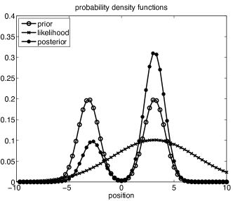
Figure 1: Displayed are the prior distribution, the likelihood from a measurement and the resulting posterior distribution. The prior as well as the posterior are bimodal Gaussian.

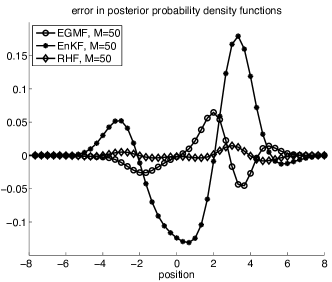
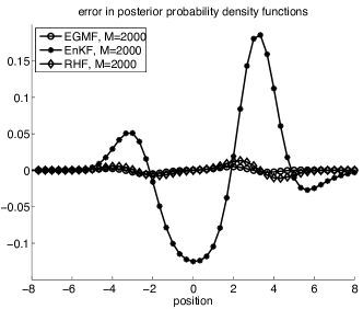
Figure 2: Numerically obtained posterior for ensemble sizes $M=50$ (left panel) and $M=2000$ (right panel). Shown are results from the EGMF, the RHF, and an EnKF analysis step. While the EGMF and the RHF converge to the correct posterior distribution, the EnKF leads to qualitatively incorrect results for both ensemble sizes.

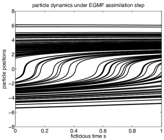
Figure 3: Displayed is the rearrangement of the particles under the dynamics of the EGMF analysis step. Rapid transitions between the Gaussian mixture components are induced by the vector field $u_{\rm B}$.

We test our formulation first for a single assimilation step where the prior is a bimodal Gaussian

$$\pi_{\rm prior}(x)=\frac{1}{2}\frac{1}{\sqrt{2\pi}}e^{-(x-\pi)^{2}/2}+\frac{1}{2}\frac{1}{\sqrt{2\pi}}e^{-(x+\pi)^{2}/2}$$ (54)

and the likelihood is

$$\pi(y_{\rm obs}|x)=\frac{1}{\sqrt{2\pi}4}e^{-(x-\pi)^{2}/32}.$$ (55)

The posterior distribution is again bimodal Gaussian and can be computed analytically. See Fig. 1. Here we demonstrate how an EnKF, the RHF, and the proposed EGMF approximate the posterior for ensemble sizes $M=50,2000$ and for $x_{i}(0)\sim\pi_{\rm prior}$, $i=1,\ldots,M$. See Fig. 2. Both the RHF and the EGMF are capable of reproducing the Bayesian assimilation step correctly for $M$ sufficiently large while the EnKF leads to a qualitatively incorrect result. The transformation of the ensemble members (particles) under the dynamics (16) is displayed in Fig. 3.

      

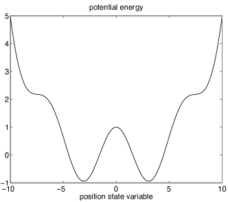
Figure 4: Shown is the potential energy $V$ used in both the Brownian and Langevin dynamics model.

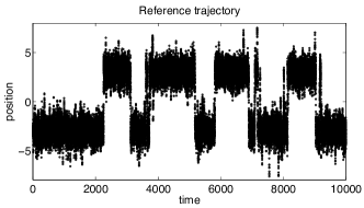
Figure 5: Shown is the reference solution from which observations are generated by adding Gaussian noise with mean zero and variance $R$.

      

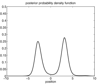
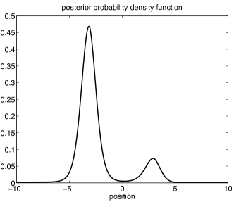
Figure 6: Displayed are two posterior PDFs for measurement error variance $R=36$ as obtained from the Fokker-Planck approach. A distinct bimodal behavior can be observed which motivates the use of a binary Gaussian mixture model for the EGMF.

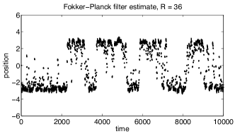
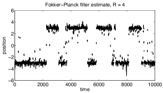
Figure 7: Estimated ensemble mean computed from a direct simulation of the assimilation problem using a discretized Fokker-Planck equation for measurement error variance $R=36$ (left panel) and $R=4$ (right panel).

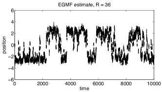
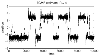
Figure 8: Ensemble mean from the EGMF for measurement error variance $R=36$ (left panel) and $R=4$ (right panel). It can be observed that the EGMF leads to results similar to those from the discrete Fokker-Planck approach (Fig. 7).

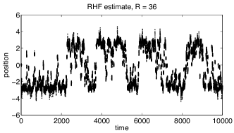
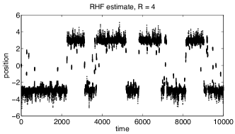
Figure 9: Ensemble mean from a RHF for measurement error variance $R=36$ (left panel) and $R=4$ (right panel). The results are for $M=50$ particles. It can be observed that the RHF leads to results similar to those from the discrete Fokker-Planck approach (Fig. 7).

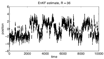
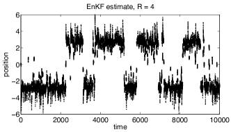
Figure 10: Ensemble mean from an EnKF with perturbed observations for measurement error variance $R=36$ (left panel) and $R=4$ (right panel). The results are for $M=50$ particles. The EnKF behaves not as well as the RHF, the EGMF, and the discretized Fokker-Planck approach. Similar results are obtained for an ensemble square root filter.

We now present results from three increasingly complex filtering problems.

5.2 A one-dimensional model problem

As a first numerical example we consider Brownian dynamics under a one-dimensional potential $V(x)$, i.e.

$${\rm d}x=-V^{\prime}(x){\rm d}t+{\rm d}w(t),$$ (56)

where $w(t)$ denotes standard Brownian motion and the potential is given by

$$V(x)=\cos(x)+\frac{3}{4}(x/6)^{4}.$$ (57)

See Fig. 4. The true reference trajectory is started at $x(0)=-3.14$. See Fig. 5. Measurements of $x(t)$ are collected every 10 time units with two different values of the measurement error variance $R$ ($R=4,36$).

The initial PDF is given by the bimodal distribution

$$\pi_{0}(x)\propto e^{-(x-3.14)^{2}/2}+e^{-(x+3.14)^{2}/2}.$$ (58)

Depending on the distribution of ensemble members we either use a single Gaussian ($L=1$) or a bi-Gaussian mixture ($L=2$) in the EGMF assimilation step. A single Gaussian is used whenever more than 90% of the particles are located near either the right (i.e. $x_{i}>0$) or left potential well (i.e. $x_{i}<0$). The computed variances are modified such that $\sigma_{l}^{2}\geq 0.0005$ to avoid singularities in the EM algorithm. The model equation (56) is discretized with the forward Euler method and time-step $\Delta t=0.1$. The total simulation interval is $t\in[0,100000]$. The assimilation equations with (42) and (43) are discretized with the forward Euler method and step-size $\Delta s=0.05$. The $l_{\infty}$-norm of $u_{\rm B}({\bf x},s)$ is limited to a value of $u_{\rm cut}=5/\Delta s$.

The performance of the EGMF is compared to an EnKF with perturbed observations, an ensemble square root filter, and a RHF. The particle positions are adjusted during each data assimilation step of a RHF such that the particles maintain equal weights $\gamma_{i}=1/M$. The adjustment is done similar to what has been proposed by Anderson (2010) except that the posterior is approximated by piecewise constant functions.

For this simple, one-dimensional problem the densities can be directly propagated through a discretization of the associated Fokker-Planck equation. Bayes theorem reduces to a multiplication of the prior PDF approximation from the Fokker-Planck approximation with the likelihood at each grid point. We have used a grid with mesh-size $\Delta x=0.125$ over $x\in[-10,10]$ to provide an independent and accurate filtering result. Periodic boundary conditions are used for the diffusion operator such that the spatial discretization leads to a stochastic matrix. It is found from the numerical simulations that $R=36$ leads to a pronounced bimodal behavior of the solution PDF $\pi$. See Figure 6 for two posterior PDF approximations from the Fokker-Planck approach.

Typical filter behaviors over the time interval $t\in[0,10000]$ with regard to the reference trajectory can be found in Figures 7, 8, 9, and 10, respectively, for $M=50$ ensemble members. The EGMF and the RHF display a behavior similar to that from the discretized Fokker-Planck approach while significantly different results are obtained from the EnKF implementation with perturbed observations. Similar results are obtained for an ensemble square root filter (not displayed). The EGMF uses a bi-Gaussian approximation in 97% of the assimilation steps for $R=36$ and in 47% of the assimilation steps for $R=4$.

We also provide the root mean square (RMS) error between the computed mean from the three different filters and the mean computed from the Fokker-Planck approach in Table 1 for $R=36$ and different ensemble sizes $M$. The RHF converges as $M\to\infty$ to the solution of the Fokker-Planck approach for this one-dimensional model problem. The EGMF provides better results than the EnKF but does not converge since the limiting distributions are not exactly bi-Gaussian. Note that the EGMF should converge for $M\to\infty$ and the number of mixture components sufficiently large. Note also that the RHF does not converge to the analytic filter solution as $M\to\infty$ in case of more than one dynamic variable (i.e. $N>1$). See also the following example.

Table 1: RMS errors for ensemble means obtained from EnKF, RHF, and EGMF compared to the expected value computed by a Fokker-Planck discretization with error variance $R=36$ and $M=20,50,100$ particles/ensemble members.

	RHF	EGMF	EnKF
$M=20$	0.6551	0.7683	1.0283
$M=50$	0.3717	0.5127	0.8798
$M=100$	0.2691	0.4033	0.8412

5.3 A two-dimensional model problem

We discuss another example from classical mechanics. The evolution of a particle with position $q\in\mathbb{R}$ and velocity $v\in\mathbb{R}$ is described by Langevin dynamics (Gardiner, 2004) with equations of motion

$$dq = v\,dt,$$ (59)

$$dv = -V^{\prime}(q)\,dt-\gamma v\,dt+\sigma dw(t),$$ (60)

where the potential $V(q)$ is given by

$$V(q)=\cos(q)+\frac{3}{4}(q/6)^{4},$$ (61)

the friction coefficient is $\gamma=0.25$, $w(t)$ denotes standard Brownian motion, and $\sigma^{2}=0.35$. A reference solution, denoted by $(q_{r}(t),v_{r}(t))$, is obtained for initial condition $(q_{0},v_{0})=(1,1)$ and a particular realization of $w(t)$.

Let us address the situation that the reference solution is not directly accessible to us and that instead we are only able to observe $Q(t)$ subject to

$$dQ(t)=v_{r}(t)\,dt+c^{1/2}d\xi(t),$$ (62)

where $\xi(t)$ denotes again standard Brownian motion and $c=0.2$. In other words, we are effectively only able to observe particle velocities.

We now combine the model equations and the observations within the ensemble Kalman-Bucy framework. The ensemble filter relies on the simultaneous propagation of an ensemble of solutions $x_{i}(t)=(q_{i}(t),v_{i}(t))\in\mathbb{R}^{2}$, $i=1,\ldots,M$. In our experiment we set $M=50$. The filter equations for an EGMF with a single Gaussian, ensemble Kalman-Bucy filter (Bergemann and Reich, 2011), respectively, become

$$dq_{i} = v_{i}\,dt-\frac{P_{qv}}{2c}(v_{i}\,dt+\bar{v}\,dt-2dQ(t)),$$ (63)

$$dv_{i} = -V^{\prime}(q_{i})\,dt-\gamma v_{i}\,dt+\sigma dw_{i}(t)-\frac{P_{vv}}{2c}(v_{i}\,dt+\bar{v}\,dt-2dQ(t))$$ (64)

with mean

$$\bar{v}=\frac{1}{M}\sum_{i=1}^{M}v_{i},\qquad\bar{q}=\frac{1}{M}\sum_{i=1}^{M}q_{i}$$ (65)

and variance/covariance

$$P_{vv}=\frac{1}{M-1}\sum_{i=1}^{M}(v_{i}-\bar{v})^{2},\qquad P_{qv}=\frac{1}{M-1}\sum_{i=}^{M}(q_{i}-\bar{q})(v_{i}-\bar{v}).$$ (66)

The equations are solved for each ensemble member with different realizations $w_{i}(t)$ of standard Brownian motion and step-size $\Delta t=0.01$. The observation interval in (62) is $\tau=\Delta t$. The extension of the EGMF to a Gaussian mixture with $L=2$ is straightforward. One substitutes $y=v$, $R=c/\Delta t$, and $y_{\rm obs}=\Delta Q(t_{n})/\Delta t$ with

$$\Delta Q(t_{n})=v_{r}(t_{n})\Delta t+\sqrt{c\Delta t}\xi_{n},\qquad\xi_{n}\sim N(0,1),$$ (67)

into (42) and (43) and sets $\Delta s=1$ in the numerical time-stepping procedure for the assimilation step. The $l_{\infty}$-norm of $u_{\rm B}({\bf x},s)$ is limited to a value of $u_{\rm cut}=0.25/\Delta s$. Assimilation is performed at every model time-step. We perform a total of two million time-steps/data assimilation cycles. In the same manner one can implement a RHF for this problem.

The computed ensemble means $\bar{q}(t)$ and $\bar{v}(t)$ in comparison to the reference solution can be found in Fig. 11 for the continuous EGMF (using $L=1$ and $L=2$ mixture components as appropriate) and the ensemble Kalman-Bucy filter (continuous EGMF with $L=1$). The root mean square (RMS) error with respect to the true reference solution is 2.3331 for the ensemble Kalman-Bucy filter and 1.9148 for the EGMF, which amounts to a relative improvement of about 20%. The EGMF uses a bi-Gaussian distribution in about 25% of the assimilation steps. For comparison we show the results from the RHF in Fig. 12 for $M=50$ particles. To interpret the behavior of the RHF one needs to look at the potential energy function $V(q)$ (see Fig. 4). The RHF assimilation scheme apparently pushes the solutions occasionally into the flat side regions of the potential energy curve resulting in a relatively large RMS error of 3.9375. Qualitatively similar results are obtained for the RHF with $M=800$ particles. Recall that we do observe velocities and not positions in this example and that the RHF uses the ensemble generated covariance matrix ${\bf P}$ to linearly regress filter increments onto state space.

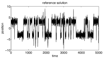
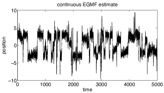
Figure 11: The reference solution $q_{r}(t)$ (left panel) and the estimated (ensemble mean) solution from the continuous EGMF (right panel) over the first quarter of the simulation interval $t\in[0,20000]$. The estimated solution mostly follows the reference solution with the exception of a number of missed transitions.

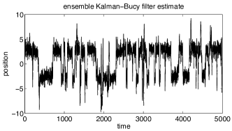
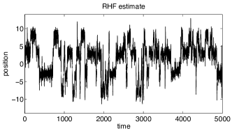
Figure 12: The estimated (ensemble mean) solution from the ensemble Kalman-Bucy filter over a quarter of the simulation interval is displayed in the left panel. The results look qualitatively similar to the results from the EGMF filter. However, in terms of RMS errors, the EGMF outperforms the ensemble Kalman-Bucy filter by about 20% over the complete simulation interval. The right panel displays the estimated (ensemble mean) solution from the RHF (left panel). The reader should note the enlarged range of the vertical axis. At several instances the filtered solution strongly deviates from the reference solution. To interpret this behavior we need to have a closer look at the potential energy $V(q)$ (compare Fig. 4). Apparently the RHF interprets the data as corresponding to solutions with positions in the flat side regions of the potential energy function.

5.4 Lorenz-63 model

The three variable model

$$\dot{x}=10(y-x),\quad\dot{y}=x(28-z)-y,\quad\dot{z}=xy-\frac{8}{3}z$$ (68)

of Lorenz (1963) is used as a final test for the EGMF method. Only the $x$ variable is observed every 0.20 time units with an observational error drawn from a normal distribution with mean zero and variance eight. The model time-step is $\Delta t=0.01$. A total of 101000 assimilation steps is performed for each experiment with only the last 100000 steps being used for the computation of RMS errors. We have implemented an ensemble square root filter, a RHF, and an EGMF using formulation (45)-(46) with ${\bf B}=c{\bf P}$, ${\bf P}$ the empirical covariance matrix of the ensemble. The parameter $c$ is chosen from the interval $c\in[0.4,1.0]$. The number of ensemble members is set to $M=25$ and no covariance localization is applied. The internal assimilation step-size is $\Delta s=1/4$ and the $l_{\infty}$-norm of $u_{\rm B}({\bf x},s)$ is limited to a value of $u_{\rm cut}=0.125/\Delta s$. We have computed the RMS errors for ensemble inflation factors between 1.0 and 1.3 and only report the optimal results in Fig. 13 as a function of $c$ for the EGMF. The overall smallest RMS error is achieved for $c=0.6$ with a value of 4.1114. The associated RMS errors for the ensemble square root filter are $4.4813$ and $4.6596$ for the RHF, respectively. An increase in the number of ensemble members to $M=100$ leads to a reduction in the RMS error for the RHF to 4.3276 while the ensemble square root filter yields its optimal performance for $M=50$ with a RMS error of 4.3785. Both values are significantly larger than the optimal RMS error for the EGMF with $M=25$. A better performance is observed for the EnKF with perturbed observations and $M=25$ for which we obtain 4.1775 as the smallest RMS error which, in fact, is close to the performance of the EGMF with $c=1$.

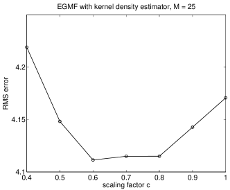
Figure 13: RMS errors from the EGMF for a range of values of the scaling parameter $c$ and ensemble size $M=25$. A series of experiments has been conducted with the Lorenz-63 model for each fixed scaling parameter $c\in[0.4,1.0]$ and a range of ensemble inflation factors. We only display the optimal results. The overall smallest RMS error is achieved for $c=0.6$ with a value of 4.1114. The corresponding optimal RMS error for an ensemble square root filter is $4.4813$ and $4.6596$ for the RHF, respectively. The EnKF with perturbed observations leads to a RMS error of $4.1775$ which is only slightly worse than the performance of the EGMF with $c=1$.

6 Summary

We have extended the popular EnKF to statistical models provided by Gaussian mixtures. The EGMF is derived using a continuous reformulation of the Bayesian analysis step and consists of a combination of EnKF steps for each mixture component and an exchange term. The exchange term is determined for each measurement by a scalar elliptic PDE, which can be solved analytically. We have demonstrated by means of two numerical examples that the EGMF performs well when bimodal PDFs arise naturally from the model dynamics. The EGMF provides a valuable and easy to implement alternative to sequential Monte Carlo methods and other nonlinear filter algorithms. In this paper, we have used the standard EM algorithm to assign Gaussian mixture models to ensemble predictions. More refined methods such as those discussed by Fraley and Raftery (2007) will be considered in future work in order to provide a robust and accurate clustering of ensemble predictions. Alternatively, one can implement the EGMF with a Gaussian kernel density estimator. In this case, the empirical covariance matrix of the ensemble can be used as a base for kernel bandwidth selection (Wand and Jones, 1995). With this choice, the EGMF becomes closely related to the RHF of Anderson (2010). The feasibility of our approach has been demonstrated for the Lorenz-63 model. Further work is required to assess the merits of Gaussian kernel density estimators in comparison to EnKF and RHF implementations for high dimensional systems. Encouraging results have also been reported by Stordal et al. (2011) for their related adaptive Gaussian mixture filter applied to the Lorenz-96 model (Lorenz, 1996; Lorenz and Emanuel, 1998).

References

- Amezcua et al. [2011] J. Amezcua, E. Kalnay, K. Ide, and S. Reich. Using the Kalman-Bucy filter in an ensemble framework. Mon. Weath. Rev., submitted, 2011.
- Anderson [2010] J.L. Anderson. A non-Gaussian ensemble filter update for data assimilation. Monthly Weather Review, 138:4186–4198, 2010.
- Anderson and Anderson [1999] J.L. Anderson and S.L. Anderson. A Monte Carlo implementation of the nonlinear filtering problem to produce ensemble assimilations and forecasts. Mon. Wea. Rev., 127:2741–2758, 1999.
- Bain and Crisan [2009] A. Bain and D. Crisan. Fundamentals of stochastic filtering, volume 60 of Stochastic modelling and applied probability. Springer-Verlag, New-York, 2009.
- Bergemann and Reich [2010a] K. Bergemann and S. Reich. A localization technique for ensemble Kalman filters. Q. J. R. Meteorological Soc., 136:701–707, 2010a.
- Bergemann and Reich [2010b] K. Bergemann and S. Reich. A mollified ensemble Kalman filter. Q. J. R. Meteorological Soc., 136:1636–1643, 2010b.
- Bergemann and Reich [2011] K. Bergemann and S. Reich. An ensemble Kalman-Bucy filter for continuous data assimilation. Meteorolog. Zeitschrift, submitted, 2011.
- Crisan and Xiong [2010] D. Crisan and J. Xiong. Approximate McKean-Vlasov representation for a class of SPDEs. Stochastics, 82:53–68, 2010.
- Dempster et al. [1977] A.P. Dempster, N.M. Laird, and D.B. Rubin. Maximum likelihood from incomplete data via the EM algorithm. J. Royal Statistical Soc., 39B:1–38, 1977.
- Evensen [2006] G. Evensen. Data assimilation. The ensemble Kalman filter. Springer-Verlag, New York, 2006.
- Fraley and Raftery [2007] Ch. Fraley and A.E. Raftery. Bayesian regularization for normal mixture estimation and model-based clustering. Journal of Classification, 24:155–181, 2007.
- Frei and Künsch [2011] M. Frei and H.R. Künsch. Mixture ensemble Kalman filters. Computational Statistics and Data Analysis, in press, 2011.
- Gardiner [2004] C.W. Gardiner. Handbook on stochastic methods. Springer-Verlag, 3rd edition, 2004.
- Hamill et al. [2001] Th.M. Hamill, J.S. Whitaker, and Ch. Snyder. Distance-dependent filtering of background covariance estimates in an ensemble Kalman filter. Mon. Wea. Rev., 129:2776–2790, 2001.
- Houtekamer and Mitchell [2001] P.L. Houtekamer and H.L. Mitchell. A sequential ensemble Kalman filter for atmospheric data assimilation. Mon. Wea. Rev., 129:123–136, 2001.
- Lorenz [1963] E.N. Lorenz. Deterministic non-periodic flows. J. Atmos. Sci., 20:130–141, 1963.
- Lorenz [1996] E.N. Lorenz. Predictibility: A problem partly solved. In Proc. Seminar on Predictibility, volume 1, pages 1–18, ECMWF, Reading, Berkshire, UK, 1996.
- Lorenz and Emanuel [1998] E.N. Lorenz and K.E. Emanuel. Optimal sites for suplementary weather observations: Simulations with a small model. J. Atmos. Sci., 55:399–414, 1998.
- Reich [2011] S. Reich. A dynamical systems framework for intermittent data assimilation. BIT, 51:235–249, 2011.
- Schaefer [1997] J.L. Schaefer. Analysis of incomplete multivariate data by simulation. Chapmann and Hall, London, 1997.
- Smith [2007] K.W. Smith. Cluster ensemble Kalman filter. Tellus, 59A:749–757, 2007.
- Stordal et al. [2011] A.S. Stordal, H.A. Karlsen, G. Nævdal, H.J. Skaug, and B. Vallés. Bridging the ensemble Kalman filter and particle filters: the adaptive Gaussian mixture filter. Comput. Geosci., 15:293–305, 2011.
- Tippett et al. [2003] M.K. Tippett, J.L. Anderson, G.H. Bishop, T.M. Hamill, and J.S. Whitaker. Ensemble square root filters. Mon. Wea. Rev., 131:1485–1490, 2003.
- Villani [2003] C. Villani. Topics in Optimal Transportation. American Mathematical Society, Providence, Rhode Island, NY, 2003.
- Wand and Jones [1995] M.P. Wand and M.C. Jones. Kernel smoothing. Chapmann and Hall, London, 1995.