On Production of ‘Soft’ Particles in Au+Au and Pb+Pb Collisions at High Energies

Abstract

Production of low-$p_{T}$ (soft) hadronic particles in high energy collisions constitutes a significant corner of special interests and problems, as the perturbative quantum chromodynamics (pQCD) does not work in this region. We have probed here into the nature of the light particle production in two symmetric nuclear collisions at two neighbouring energies with the help of two non-standard models. The results are found to be in good agreement with data. Despite this, as the models applied here are not intended to provide deep insights into the actual physical processes involved in such collisions, the phenomenological bounds and constraints which cannot be remedied for the present continue to exist.

Keywords: Relativistic heavy ion collision, Inclusive production with identified hadrons, Inclusive Cross-section, Meson production

PACS nos.: 25.75.-q, 13.85.Ni, 13.60.Hb, 13.60.Le

1 Introduction

Multiple production of hadrons at high energies, named also multiparticle production phenomena, is still not at all a well-understood sector. In general, the largest bulk of the particles produced in nature, called secondaries, is detected to be of the small transverse momenta, though in arranged laboratory collisions at colliders (inclusive of LHC) the particles are, in the main, detected with and reported for large transverse momenta. The theoretical studies based on the standard model(SM) of particle interaction are grounded on an artificial division between ’soft’(low-$p_{T}$) and ’hard’(large-$p_{T}$) regions. The latter wherein the perturbative techniques are applied is called Perturbative Quantum Chromodynamics (pQCD); and the former wherein perturbation theory fails is termed non-perturbative domain. And most of the particles in nature as well as in laboratory collisions fall under this non-perturbative sector, for whom there is no widely acceptable general theory[1]. Our interest in the present work is focussed on particle production at low-$p_{T}$ valued $Pb+Pb$ interaction at relatively lower SPS energies. The prime object of this paper is to study the $p_{T}$-dependence of the invariant cross-sections for main vaieties of hadron secondaries with the help of one or two models which do not typically fall under the Standard variety and which will be outlined in the next section. The main species (like kaon, pion, proton) of the secondaries here are pions, kaons and proton-antiproton produced in both lead-lead interactions at $\sqrt{S_{NN}}$=17.3GeV and $E_{lab}$=20A, 30A, 40AGeV and Au+Au reactions at RHIC at $\sqrt{S_{NN}}$=19.6GeV.

In our approach we would try (i) to demolish the artifact of soft-hard division and try to apply a unified outlook by treating the production of particles on a uniform footing.(ii) to check whether the outlook of the divide between the exponentialisation and the power-law nature based on the artificial soft-hard boundary is of any real merit or worth and in probing this point we have been spurred on to by a very recent report published by Busza[2] with emphasis on the first lesson to be learnt from PHOBOS Collaboration that there is no anomalous production of low-$p_{T}$ (Soft) particles at RHIC; (iii) to study how the nature of $p_{T}$-scaling in the particle production scenario manifests itself in the extreme case of low-$p_{T}$ and the relatively lower side of the high energy domain i.e., at SPS region.

The work to be reported here aims at putting a strong question-mark to the time honoured contention of the large bulk of the high energy physicists that the data on ‘soft’ collisions could be described by the exponential models; the power laws are applicable for explaining the data on ‘hard’ collisions. In fact, in this work we have contested this view and have attempted at showing that power laws could be applied almost universally.

The organisation of the work is as follows. In Section-2 we present a brief outline of the very simple theoretical frameworks. The Section-3 embodies the results of the work in graphical plots, and tables which show up the used values of the parameters. In Section-4 we have discussed in detail the very minute points that worked in arriving at the desired results and had provided answers to some anticipatory and probable questions from the readers. The last section offers precisely the summary and outlook.

2 Outlines of the Theoretical Framework

This section is divided into subsections comprising the (i) Power-law-based $p_{T}$-scaling Model (also named Hagedorn Model) and (ii) The Combinational Approach, both of which are very much in use in recent times by some of us

2.1 Hagedorn Model : Essentially a Power Law with $p_{T}$-scaling

Our objective here is to study the inclusive $p_{T}$-spectra of the various secondaries of main varieties produced in $pp$ collisions. The kinematics of an inclusive reaction $h_{a}h_{b}$$\longrightarrow$$hX$ is described by Lorentz invariants. These are e.g. the center-of-mass energy squared s = ($P_{a}$+$P_{b}$)², the transverse momentum transverse (squared) t = ($P_{h}$-$P_{a}$)² and the missing mass $M_{X}$, where $M_{X}$ is the mass of the undetected components that are produced in the reaction process, denoted by ‘X’ in $h_{a}h_{b}$$\longrightarrow$$hX$. It is common to introduce the dimensionless variables (u = $M_{X}$²-s-t),

$$x_{1}=-\frac{u}{s},x_{2}=-\frac{t}{s}$$ (1)

where s,t,u are called Mandelstam variables. These variables are related to the rapidity y and radial scaling factor, $x_{R}$ of the observed hadron by

$$y=\frac{1}{2}log(x_{1}/x_{2})$$ (2)

$$x_{R}=\frac{2|\overrightarrow{p_{cm}}|}{\sqrt{s}}=1-\frac{M_{X}^{2}}{s}=x_{1}+x_{2}$$ (3)

Since most of existing data are at y = 0 where $x_{R}$ = $x_{T}$ = 2$p_{T}$/$\sqrt{s}$ and $|\overrightarrow{p_{cm}}|$ is just the magnitude of the three momentum in c.m. system, one often refers to the scaling of the invariant cross section as ”$x_{T}$ scaling”. For y$\neq$0, we find the variable $x_{R}$ more useful than $x_{T}$, since $x_{R}$ allows a smooth matching of inclusive and exclusive reactions in the limit $x_{R}$ $\longrightarrow$ 1.

We will assume that at high $p_{T}$, the inclusive cross section takes a factorized form. And one such a factorized form was given by Back et al[3].

$$\frac{dN}{dp_{T}}=\frac{p_{T}(n-2)(n-1)}{{p_{0}}^{2}}(1+\frac{p_{T}}{p_{0}})^{-n}$$ (4)

where n and $p_{0}$ are adjustable parameters. The values of the exponent n are just numbers. $p_{0}$ is to be viewed as a energy-band dependent critical value of the transverse momentum within the low-$p_{T}$ limits and is introduced for the sake of making the term within the parenthesis dimensionless, thus lending the expression within the parenthesis a scaling form with $p_{T}/p_{0}$, called $p_{T}$-scaling.

With the simplest recasting of form the above expression (4) and with replacements like $p_{T}$=x, $p_{0}$=q, C = a normalisation factor, and in the light of the definitions of the inclusive cross-sections, we get the following form as the final working formula

$$z=f(x)=\frac{C}{q^{2}}(1+\frac{x}{q})^{-n}$$ (5)

2.2 Combinational Approach : De-Bhattacharyya Model

The combinational approach outlines a method for arriving at the results to be obtained on some observables measured in particle-nucleus or nucleus-nucleus interactions at high energies from those obtained for the basic nucleon-nucleon (or proton-proton) collision. And the results for nucleon-nucleon interactions are based on power-law fits which are assumed to be physically understood somewhat fairly in the light of both thermal model and/or pQCD-related phenomenology. So, essentially this represents a notional combination of power law model for pp reactions and the the introduction of some mass number-dependent product term signifying the nuclear effects on invariant cross-sections, from which the name ‘Combinational Approach’ is derived. And this notional combination subsumes the property of factorization which is one of the cardinal principles in the domain of particle physics.

The expression for the transverse momentum-dependence of the inclusive cross-section for secondary particle, Q, produced in nucleus-nucleus(AB) collisions is given by[4]-[7]

$$E\frac{d^{3}\sigma}{dp^{3}}|_{AB\rightarrow QX}\sim(AB)^{f(p_{T})}E\frac{d^{3}\sigma}{dp^{3}}|_{pp\rightarrow QX}$$ (6)

Where A and B on the right-hand side of the above equation stand for the mass numbers of two colliding nuclei; the term, $E\frac{d^{3}\sigma}{dp^{3}}|_{pp\rightarrow QX}$ is the inclusive cross section for production of the same secondary,Q,in pp or $p\overline{p}$ collision at the same (center-of-mass) c.m. energy.

The nature of ($p_{T}$)-dependence of the inclusive cross-section term, $E\frac{d^{3}\sigma}{dp^{3}}|_{pp\rightarrow QX},$ occurring in eqn.(1), for production of a Q-species in $pp/p\overline{p}$ reactions at high energies is taken here in the form of a power-law as was initially suggested by G.Arnison et al.[8]:

$$E\frac{d^{3}\sigma}{dp^{3}}|_{pp\rightarrow QX}\approx C_{1}(1+\frac{p_{T}}{p_{0}})^{-n}$$ (7)

Where $C_{1}$ is the normalization constant; and $p_{0}$ and n are two interaction-dependent parameters for which the values are to be obtained by fitting the pp and $p\overline{p}$ data at various energies. Of course, such a power-law form was applied to understand the nature of the transverse momentum spectra of the pion secondaries by some other authors[9]-[12] as well.

Hence including eqn. (7) and a parametrization for the factor, $f(p_{T})$, into eqn. (6), the final working formula is given by[4]-[7]

$$E\frac{d^{3}\sigma}{dp^{3}}|_{AB\rightarrow QX}\approx C(AB)^{(\alpha p_{T}-\beta p^{2}_{T})}(1+\frac{p_{T}}{p_{0}})^{-n}$$ (8)

Where C,$\alpha$ and $\beta$ are constants and have to be determined by fitting the measured data on ($p_{T}$)-spectra for production of charged hadrons in nucleus-nucleus collisions at high energies. Some sort of physical interpretations for $\alpha$ and $\beta$ are given in some of our previous works[5],[6].

A useful way[3],[13] to compare the spectra from nucleus-nucleus collisions to those from nucleon-nucleon collisions is to scale the normalized pp (or $p\overline{p}$)spectrum (assuming the value of inelastic pp cross-section, $\sigma^{pp}_{inel}\approx$ 41 mb) by the number of binary collisions,$\langle N_{coll}\rangle$, corresponding to the centrality cuts applied to the nucleus-nucleus spectra and construct the ratio. This ratio is called the nuclear modification factor, $R_{AB}$, which is to be expressed in the form

$$R_{AB}=\frac{\frac{1}{\langle N_{coll}\rangle}E\frac{d^{3}N}{dp^{3}}|_{AB}}{\frac{1}{\sigma^{PP}_{inel}}E\frac{d^{3}\sigma}{dp^{3}}|_{PP}}$$ (9)

It is to be noted here that both the numerator and the denominator of equation (9) contain a term of the form $(1+\frac{p_{T}}{p_{0}})^{-n}$which gives the $p_{T}$-dependence of the hadronic-spectra produced in basic ($pp/p\overline{p}$)collision. And as the other terms like, $\langle N_{coll}\rangle,\sigma^{pp}_{inel}$ are constants for a specific interaction at a definite energy and fixed centrality, we can obtain by combining eqn.(8) and (9) the final expression for the ratio value in the following form :

$$R_{AB}\propto(AB)^{(\alpha p_{T}-\beta p^{2}_{T})}$$ (10)

The above steps provide the operational aspects of the combinational approach (CA). But, this approach outlines a method for arriving at the result to be obtained on some observables measured in particle-nucleus or nucleus-nucleus interactions at high energies from those obtained exclusively for only the basic nucleon-nucleon (or proton-proton)collision.And results for nucleon-nucleon collisions are based on power-law form (eqn.(7)) which is supposed here to be fairly physically understood in the light of both thermal model and/or pQCD-related phenomenology. Besides, if the data sets on a specific observable are measured in pp reactions at five or six different high energies at reasonably distant intervals, the pure parameter-effects on $p_{0}$ and n could be considerably reduced and we may build up a methodology for arriving at $p_{0}$ and n values at any other different energy by drawing the graphical plots of $p_{0}$ versus $\sqrt{S}$ and n versus $\sqrt{S}$ curves, as are done in some of our previous works[4],[5]. And on this supposition of availability of data in PP reactions at certain intervals of energy values, the number of arbitrary parameters for NA or AA collisions is reduced to only three which offer us quite a handy, useful and economical tool to understand the various aspects of the data characteristics.

The $p_{0}$ and n values in eqn. (7) represent the contributions from basic NN (PP OR $p\overline{p}$) collision at a particular energy. The values of $p_{0}$ and n are to be obtained from the expressions and plots shown in the work of De et al[4],[5]. The relevant expressions are

$$p_{0}(\sqrt{S_{NN}})=a+\frac{b}{\sqrt{\frac{S_{NN}}{GeV^{2}}}\ln(\sqrt{\frac{S_{NN}}{GeV^{2}}})}$$ (11)

$$n(\sqrt{S_{NN}})=a^{\prime}+\frac{b^{\prime}}{\ln^{2}(\sqrt{\frac{S_{NN}}{GeV^{2}}})}$$ (12)

The values of the parameters $a$, $a^{\prime}$, b and $b^{\prime}$ for different secondaries are taken from Ref.[7]. The empirically proposed nature of the plots based on eqn. (11) and eqn. (12) against the data-sets, have also been presented for $\pi^{\pm}$, $K^{\pm}$ and $p^{\pm}$ production separately in a subsequent section (Section 4).

3 Results

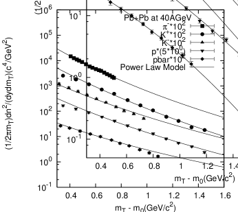
Figure 7: Transverse mass spectra of $K^{+}$, $K^{-}$, $p$, $\overline{p}$ and $\pi^{-}$ produced in central Pb+Pb Collision at 40A GeV. The lines are fits of equation of DBP Model [Left Figure] and Power Law Model [Right Figure]. The statistical errors are smaller than the symbol size, for which no errors are shown in the figure. Data are taken from [22].

In order to attain the comparability of the results obtained at various energies, we have, at the very beginning, converted all the relevant energies (with laboratory energies) into the c.m. system. And they have been presented in a tabular form as is given in Table 1. The results are presented here in graphical plots and the accompanying tables for the values of the used parameters. In Fig.(1a) and Fig.1(b) the differential cross-sections for negative and positive pion, kaon and proton-antiproton production cases in Pb+Pb collisions at SPS energies are reproduced by the used empirical parametrizations given in expressions (4) and (7). The parameter values used to obtain the model-based plots are shown in Table-2. The figures in all the cases have been appropriately labeled and the parameters are shown in the tables as mentioned in the text for each case. The data are obtained at such low-$p_{T}$ values and at the relatively lower side of the high energy in terms of $m_{T}$-values, instead of $p_{T}$ values. The relationship between $m_{T}$ and $p_{T}$ is generally given by $m_{T}^{2}$=$m_{h}^{2}+p_{T}^{2}$. Within the low-$p_{T}$ limits and for the low-mass particles ($m_{h}\ll p_{T}$) produced in any high energy collisions $m_{T}$$\approx$$p_{T}$. As the measured data are obtained and exhibited with $m_{T}$ in the abscissa we choose to retain them intact; the ordinate-observable too is kept thus undisturbed. The plots in Fig.2(a) and Fig.2(b) are for positive and negative pion, positive and negative kaon in Pb+Pb collisions at 30A GeV and the corresponding parameters are depicted in Table-3. The plots presented in Fig.(2c) for proton-antiproton production in lead-lead interaction at SPS energies, specifically at 17.3 GeV and the corresponding parameters are depicted in Table-3. The graphs in Fig.3 and Fig.4 present the results for the secondaries $\pi^{\pm}$, $K^{\pm}$ and proton-antiproton produced in the Au+Au collisions at 19.6 GeV. Used parameter values for these two figures are given in Table-4. The rest of the figures demonstrated in the Fig.5, Fig.6, Fig.8 and Fig.9 are for collisions as labelled and are based on the De-Bhattacharyya model for the major varieties of hadronic secondaries produced at four very close energies as mentioned in each of the figures separately. The parameter values used to obtain the nature of fits are shown in Table-5,6,9. The graph plotted in Fig.7 are based on both Power Law Model and DBP Model respectively, at 40A GeV in Pb+Pb collsions. The parameter values obviously remain the same as given in table-7 and Table-8.

The graphs plotted in Fig. 10(a) and Fig. 11(a) are based on Power Law Model and DBP Model respectively; they represent the fits to the invariant $p_{T}$-spectra for production of the main varieties of secondaries in 19.6 GeV Au+Au collisions at mid-rapidity and at the range of 0-10% centrality which covers the highest centrality region of nuclear collisions. The parameter values used are given in Table-10 and Table-11. The rest of the plots in Fig. 10 and Fig. 11 are for the nature of the charge-ratios-behaviours for the specific variety of the secondary particles. The Fig. 10(b), Fig. 10(c) and Fig. 10(d) are drawn on the basis of the Power Law Model; and the plots shown in Fig. 11(b), Fig. 11(c) and Fig. 11(d) are on the basis of the DBP model for the same set of charge-ratios.

At last, even on the basis of a very few four close-ranging energies and on an approximation that the measured data-values on Pb+Pb and Au+Au at the neighboring would not differ too much, we have tried to check here the merits of the phenomenological energy-dependences proposed by us in eqns. (11), (12) of the two key parameters, viz, $p_{0}$ and n. In Fig. 12 to Fig. 14 we have plotted the parameter values $p_{0}$ along the Y-axis with the energy-values as the corresponding X-axis. The dotted curves in all these figures depict the nature of the parameters obtained by the proposed empirical expressions represented by eqns. (11) and (12). The phenomenologically formulated expressions reproduce fairly well the nature of fit-values used for the two parameters. Despite the limitations pointed here out before and some others, the agreements are modestly encouraging.

4 General Discussion and Some Specific Points

By all indications, the results manifested in the measured data on the specific observables chosen here are broadly consistent with both the approaches put into work here. This is modestly true of even the nature of charge-ratios which provide virtually a cross-check of the models utilised here. Of course, at this point let us make some comments on our model-based plots, especially the plots on the charge-ratios . This is not very surprising in the sense that the De-Bhattacharyya phenomenology (DBP) through a parametrization is also essentially a power law model with a bare A-dependence, while in the pure power law model any of the chosen parameters absorb the nuclear-dependence. Still, the DBP-model inducts some physical postulates which are as follows :(i) It is assumed that the inclusive cross section of any particle in a nucleus-nucleus (AB) collision can be obtained from the production of the same in nucleon-nucleon collisions by multiplying by a product of the atomic numbers of each of the colliding nuclei raised to a particular function, $\epsilon(y,p_{T})$, which at first is unspecified (Equation 6), (ii) Secondly, we have accepted that factorization [14] of the function $\epsilon(y,p_{T})$ = $f(y)g(p_{T})$ which helps us to perform the integral over $p_{T}$ in a relatively simpler manner, (iii) Finally, we have based on the ansatz that the function f(y) can be modeled by a quadratic function with the parameters $\alpha$ and $\beta$ (Equation 10). They are to be tested in the high energy experiments of the future generations. Besides, the present DBP-based approach to deal with the data advances a systematic methodical approach in which the main parameters could be determined and ascertained, if and only if, measured laboratory data of higher accuracy and precision are available at different energies in a regular and successive interval. So, the lack of predictivity of the used two models is caused only by the circumstances, i.e. the lack of measured data at the successive and needed intervals ; the problem can be remedied by supplying the necessary and reliable data from the arranged laboratory experiments at high - to - very high energies. However, the problem of constraining the parameters still remains. The other observations are : as is expected for two symmetric collisions of neighbouring values of mass numbers at very close energies, the measured data do not reveal any significant differences with respect to the observables chosen by the experimental groups. This work demonstrates somewhat convincingly that the power law models can easily take care of data even for very low-$p_{T}$ (soft) collisions; so the notion of compartmentalisation between the possible applicability of the power law models and of the exponential models is only superficial. Besides, the power law models which establish them as more general ones obtain a clear edge over the exponential models. Reliable data on various other related observables are necessary for definitive final conclusions. By all indications, the experimentally observed nature of $p_{T}$- scaling is found to remain valid even in the studied low-$p_{T}$ range of this paper. The deeper physical implications of this work have implicity been pointed out in the last two paragraphs of the Section 1 of this work, wherein we made very clear and categorical statements on our intentions, purposes and the prime objectives. So, in order to avoid repetitions, we refrain ourselves here very carefully from commiting a rehash of the same. However, let us now try to pinpoint below some physical points and considerations which provide the necessary underpinning of the power law models.

The wide and near successful applications of the various forms of power laws have, by now, grown almost universal in almost all the branches of physics as well as in other branches of sciences. Speaking in the most general and scientific terms, the processes which are complex, violent and dissipative contributing to the non-equilibrium phenomena do generally subscribe to the power laws. The used power law behaviors are commonly believed to be the “manifestations of the dynamics of complex systems whose striking feature is of showing universal laws characterized by exponents in scale invariant distributions that happen to be basically independent of the details in the microscopic dynamics[15]”. Now let us revert from the general to the particular case(s) of high energy particle-particle, particle-nucleus or nucleus collisions. For purely hadronic, hadronuclear or nuclear interactions one of the basic features is : irrespective of the initial state, agitations caused by the impinging projectile (be it a parton or a particle/nucleon) generate system effects of producing avalanches of new kind of partons [called quark(s)/gluon(s)/any other(s)] which form an open dissipative system. The avalanches caused by production of excessive number of new partons give rise to the well-known phenomenon of jettiness of particle production processes and of cascadisation of the particle production processes leading to the fractality as was shown in a paper by Sarcevic[16]. These cascades are self-organizing, self-similar and do just have the fractal behavior. Driven by the physical impacts of these well-established factors, in the high energy collision processes do crop up the several power-laws. And how such power laws do evolve from exponential origins or roots is taken care of by the induction of Tsallis entropy[17] and a generalisation of Gibbs-Boltzmann statistics for long-range and multifractal processes. Following Sarcevic[16] the relationship between/among cascadisation, self-similarity and fractality is/was evinced in a paper[18] by a set of the present authors. In this paper we have, once more, tried to examine the worth and utility of such power laws as have been advocated here.

In the data-plots of Fig. 3(a) we observe some differences between the trends of WA98 data and the others. But it is to be noted that the data in WA98 experiment is for the observation of neutral pions, whereas our plot is intended to be one of the charged varieties of pions, e.g., $\pi^{+}$ detected at the experimental energy 17.3 GeV in c.m. system; besides, the STAR data was measured at 19.6 GeV (c.m.). This apart, in the WA98 experiment the observable along the Y-axis was just $E\frac{d^{3}\sigma}{dp^{3}}$, whereas for the others the Y-axis was described to be $\frac{1}{2\pi}\frac{d^{2}n}{m_{T}dm_{T}dy}$. The data from WA98 took up values of $m_{T}-m_{0}$ from 1 to 4 GeV/c. But all the other plots were limited to just $m_{T}-m_{0}$=1 GeV/c. So there are a host of factors of differences between WA98 data and the rest. The differences in the magnitudes of the $\pi^{+}$ plots in the invariant cross section between various data-sets might be a cumulative effect of all the above-mentioned factors.

Quite spectacularly, in fig. 3(d) for production of $K^{-}$, the differences between the data-points measured by WA98 and the rest are surely non-negligible. So the existence of discrepancy to a certain degree cannot be denied altogether.

However, one must note that the observable plotted as ordinate in the WA98 experiment is a bit different from the others, where does occur a term, denoted by $N_{evt}$ related with both statistical and systematic uncertainties, though the uncertainties in all other cases (i.e., for non-WA98) the errors are only statistical. Our guess is : the twin factors of systematic uncertainties and the separate y-observable [in the WA98] along the ordinate are responsible for introducing such differences as are shown in data-plot of Fig. 3(d). The reason(s) might be something else as well.

We observe that the data points on invariant cross-sections for production of protons show relatively much slower fall with $m_{T}$ ($p_{T}$) than the other prime varieties of hadrons. Thus one might have doubts on the accuracy of data-measurements and recordings for protons. If this is too unlikely to be the case, we guess that in the detection/measurement process the part of the ‘leading’ protons has disguised themselves and appeared as the product proton-particles enhancing protonic invariant cross-section for which the fall in the invariant cross-section with $m_{T}$ is much less. Uptil now, this explanation is certainly just tentative.

In the end, one more comment is in order. Quite knowingly, we have used here the usual binned $\chi^{2}$-method with the attending limitations of this approach to check the goodness-of-fit of our results to the data, as unbinned multivariate goodness-of-fit tests[19] have not yet gained much ground in the High Energy Physics (HEP) sector.

5 Concluding Remarks

Let us we present here very precisely the main conclusions of this work. Firstly, for these limited sets of data on production of soft particles in high energy collisions which have, so far, defied explanation, we have attempted to provide two alternative theoretical/phenomenological approaches for their interpretation in modestly successful manners. Secondly, in fact, these two approaches conceptually and inwardly are somewhat interlinked, for which limited successes of both of them are not very surprising. Thirdly, power law models are seen to act much better here than all other models; besides, they are much more general than the others. Fourthly, the applications of power law models are quite widespread in the different fields of physics in particular and of science in general, for which active interests in investigating the origin of these power laws have been aroused. And this has, so far, given rise to, in the main, two parallel streams of thought, of which one is the cascadisation phenomena and fractal mechanisms; and the other is the science of nonequilibrium phenomena that are generally probed by applying the Tsallis entropy and Tsallis statistics[20]. Confirmation of such multiple educated guesses can be made only by further dedicated researches in these fields.

At last, in response to what we learn very precisely from this work we submit the following few points: (i) Our unquestioned belief in and reliance on the Standard Model(SM) have, so far, been virtually ’regimented’, for which we fail to think of any other avenues and accept the singularity and uniqueness phenomena of the SM as taken for granted. (ii) In the sphere of surely very limited sets of data we explore and assess here the potential of two alternative models in explaining the observed data. (iii) And as we have succeeded in our attempts to a considerable extent, in our opinion, these two models dealt herewith could in future be viewed and projected as possible alternative approaches to explain the nature of observed and measured data-sets on ‘soft’ production of particle in high energy collisions.

Acknowledgements

The authors express their deep indebtedness to the learned referees for some encouraging remarks, constructive comments and valuable suggestions which helped a lot in improving an earlier version of the manuscript.

Table 1: Conversion of energy system

Beam Energy	$20AGeV$	$30AGeV$	$40AGeV$
$\sqrt{S_{NN}}$	$6.3GeV$	$7.6GeV$	$8.7GeV$

Table 2: Numerical values of the fit parameters of power law equation for $Pb+Pb$ Collisions.

Beam Energy	$Products$	$c$	$q(GeV/c)$	$n$	$\frac{\chi^{2}}{ndf}$
$20AGeV$	$\pi^{-}$	$43.935\pm 0.015$	$1.197\pm 0.037$	$10.010\pm 0.234$	$0.612/7$
$20AGeV$	$\pi^{+}$	$38.950\pm 0.233$	$1.178\pm 0.087$	$9.410\pm 0.531$	$2.628/6$
$20AGeV$	$K^{-}$	$1.690\pm 0.013$	$2.404\pm 0.014$	$14.003\pm 0.054$	$0.806/4$
$20AGeV$	$K^{+}$	$5.515\pm 0.136$	$2.001\pm 0.022$	$11.888\pm 0.180$	$4.894/4$
$20AGeV$	$p$	$3.568\pm 0.062$	$2.757\pm 0.138$	$8.006\pm 0.352$	$0.904/4$

Table 3: Numerical values of the fit parameters of power law equation for $Pb+Pb$ Collisions.

Beam Energy	$Products$	$c$	$q(GeV/c)$	$n$	$\frac{\chi^{2}}{ndf}$
$30AGeV$	$\pi^{-}$	$52.202\pm 0.307$	$1.158\pm 0.073$	$9.232\pm 0.438$	$1.158/5$
$30AGeV$	$\pi^{+}$	$47.041\pm 0.637$	$1.344\pm 0.211$	$10.026\pm 1.166$	$5.790/8$
$30AGeV$	$K^{-}$	$2.551\pm 0.040$	$2.001\pm 0.021$	$11.240\pm 0.115$	$3.519/3$
$30AGeV$	$K^{+}$	$8.962\pm 0.341$	$1.999\pm 0.017$	$12.986\pm 0.293$	$3.697/4$
$17.3GeV$	$p$	$15027.3\pm 34.99$	$2.047\pm 0.0001$	$8.504\pm 0.011$	$1.252/4$
$17.3GeV$	$\overline{p}$	$0.450\pm 0.042$	$0.439\pm 0.049$	$3.999\pm 0.037$	$1.338/5$

Table 4: Numerical values of the fit parameters for pion, kaon, proton and antiproton using Power Law Model for $Au+Au$ collisions at 19.6GeV.

Beam Energy	$Products$	$c$	$q(GeV/c)$	$n$	$\frac{\chi^{2}}{ndf}$
$19.6GeV$	$\pi^{+}$	$12.588\pm 0.183$	$0.559\pm 0.061$	$5.547\pm 0.358$	$6.518/7$
$19.6GeV$	$\pi^{-}$	$13.443\pm 0.089$	$2.001\pm 0.011$	$13.192\pm 0.065$	$27.759/29$
$19.6GeV$	$K^{+}$	$1.455\pm 0.017$	$2.002\pm 0.256$	$9.803\pm 0.109$	$13.526/11$
$19.6GeV$	$K^{-}$	$0.742\pm 0.007$	$6.640\pm 0.038$	$29.998\pm 0.050$	$27.027/18$
$19.6GeV$	$p$	$1.995\pm 0.027$	$0.887\pm 0.103$	$4.257\pm 0.233$	$18.933/11$
$19.6GeV$	$\overline{p}$	$0.188\pm 0.005$	$2.440\pm 0.057$	$7.001\pm 0.044$	$2.741/06$

Table 5: Numerical values of the fit parameters of DBP equation for $Pb+Pb$ Collisions.

Beam Energy	$Products$	$c$	$\alpha$	$\beta$	$\frac{\chi^{2}}{ndf}$
$20AGeV$	$\pi^{-}$	$1608.85\pm 18.320$	$0.020\pm 0.008$	$0.004\pm 0.010$	$20.330/12$
$20AGeV$	$\pi^{+}$	$1492.27\pm 61.830$	$0.031\pm 0.017$	$0.018\pm 0.018$	$19.790/10$
$20AGeV$	$K^{-}$	$35.667\pm 0.151$	$0.202\pm 0.010$	$0.083\pm 0.010$	$9.847/4$
$20AGeV$	$K^{+}$	$94.412\pm 2.063$	$0.334\pm 0.013$	$0.211\pm 0.014$	$2.456/3$
$20AGeV$	$p$	$11.309\pm 4.938$	$0.522\pm 0.106$	$0.142\pm 0.066$	$2.148/4$

Table 6: Numerical values of the fit parameters of DBP equation for $Pb+Pb$ Collisions.

Beam Energy	$Products$	$c$	$\alpha$	$\beta$	$\frac{\chi^{2}}{ndf}$
$30AGeV$	$\pi^{-}$	$1707.12\pm 18.260$	$0.059\pm 0.007$	$0.029\pm 0.009$	$21.159/12$
$30AGeV$	$\pi^{+}$	$1697.79\pm 27.510$	$0.050\pm 0.002$	$0.026\pm 0.004$	$24.543/15$
$30AGeV$	$K^{-}$	$45.951\pm 1.407$	$0.302\pm 0.013$	$0.181\pm 0.013$	$15.312/12$
$30AGeV$	$K^{+}$	$104.667\pm 2.330$	$0.373\pm 0.011$	$0.244\pm 0.012$	$5.078/5$
$17.3GeV$	$p$	$10.352\pm 0.070$	$0.654\pm 0.002$	$0.121\pm 0.001$	$0.635/8$
$17.3GeV$	$\overline{p}$	$6.084\pm 0.121$	$0.723\pm 0.009$	$0.281\pm 0.009$	$2.259/8$

Table 7: Numerical values of the fit parameters for negative pion, positive and negative kaon, proton and antiproton using DBP Model for $Pb+Pb$ collisions at 40A GeV.

Beam Energy	$Products$	$c$	$\alpha$	$\beta$	$\frac{\chi^{2}}{ndf}$
$40AGeV$	$\pi^{-}$	$1302.44\pm 9.467$	$0.079\pm 0.008$	$0.065\pm 0.012$	$0.109/15$
$40AGeV$	$K^{+}$	$108.27\pm 0.428$	$0.220\pm 0.002$	$0.090\pm 0.003$	$0.328/13$
$40AGeV$	$K^{-}$	$44.963\pm 0.323$	$0.200\pm 0.005$	$0.093\pm 0.006$	$0.099/13$
$40AGeV$	$p$	$80.879\pm 1.260$	$0.346\pm 0.007$	$0.109\pm 0.006$	$0.638/14$
$40AGeV$	$\overline{p}$	$0.599\pm 0.004$	$0.382\pm 0.005$	$0.145\pm 0.006$	$0.129/14$

Table 8: Numerical values of the fit parameters for negative pion, positive and negative kaon, proton and antiproton using Power Law Model for $Pb+Pb$ collisions at 40A GeV.

Beam Energy	$Products$	$c$	$q(GeV/c)$	$n$	$\frac{\chi^{2}}{ndf}$
$40AGeV$	$\pi^{-}$	$54.328\pm 1.296$	$1.198\pm 0.022$	$10.003\pm 0.042$	$0.103/15$
$40AGeV$	$K^{+}$	$9.176\pm 0.166$	$1.999\pm 0.007$	$13.856\pm 0.132$	$0.617/07$
$40AGeV$	$K^{-}$	$2.429\pm 0.067$	$1.734\pm 0.048$	$10.031\pm 0.210$	$1.114/11$
$40AGeV$	$p$	$12.827\pm 0.589$	$1.629\pm 0.043$	$10.002\pm 0.070$	$0.433/08$
$40AGeV$	$\overline{p}$	$0.078\pm 0.002$	$1.382\pm 0.054$	$7.022\pm 0.178$	$0.800/08$

Table 9: Numerical values of the fit parameters for pion, kaon, proton and antiproton using DBP Model for $Au+Au$ collisions at 19.6GeV.

Beam Energy	$Products$	$c$	$\alpha$	$\beta$	$\frac{\chi^{2}}{ndf}$
$19.6GeV$	$\pi^{+}$	$223.493\pm 28.050$	$0.239\pm 0.037$	$0.100\pm 0.027$	$4.202/6$
$19.6GeV$	$\pi^{-}$	$352.948\pm 12.490$	$0.113\pm 0.006$	$0.029\pm 0.002$	$3.292/5$
$19.6GeV$	$K^{+}$	$22.951\pm 0.709$	$0.350\pm 0.014$	$0.168\pm 0.015$	$9.672/8$
$19.6GeV$	$K^{-}$	$13.611\pm 0.041$	$0.287\pm 0.005$	$0.110\pm 0.006$	$19.681/19$
$19.6GeV$	$p$	$7.030\pm 0.044$	$0.648\pm 0.004$	$0.168\pm 0.006$	$15.994/14$
$19.6GeV$	$\overline{p}$	$0.557\pm 0.021$	$0.649\pm 0.024$	$0.297\pm 0.032$	$4.117/4$

Table 10: Numerical values of the fit parameters for pion, kaon, proton and antiproton using Power Law Model for $Au+Au$ collisions at 19.6GeV for 0-10% centrality.

Beam Energy	$Products$	$c$	$q(GeV/c)$	$n$	$\frac{\chi^{2}}{ndf}$
$19.6GeV$	$\pi^{+}$	$18.522\pm 0.520$	$0.592\pm 0.019$	$6.689\pm 0.156$	$20.538/13$
$19.6GeV$	$\pi^{-}$	$15.410\pm 0.302$	$0.658\pm 0.026$	$6.834\pm 0.216$	$13.235/13$
$19.6GeV$	$K^{+}$	$1.686\pm 0.028$	$1.833\pm 0.070$	$8.648\pm 0.234$	$0.841/19$
$19.6GeV$	$K^{-}$	$0.999\pm 0.039$	$1.999\pm 0.032$	$9.123\pm 0.264$	$0.700/12$
$19.6GeV$	$p$	$1.672\pm 0.016$	$1.567\pm 0.025$	$6.587\pm 0.066$	$10.212/16$
$19.6GeV$	$\overline{p}$	$0.159\pm 0.002$	$1.568\pm 0.018$	$6.587\pm 0.052$	$8.980/21$

Table 11: Numerical values of the fit parameters for pion, kaon, proton and antiproton using DBP Model for $Au+Au$ collisions at 19.6GeV for 0-10% centrality.

Beam Energy	$Products$	$c$	$\alpha$	$\beta$	$\frac{\chi^{2}}{ndf}$
$19.6GeV$	$\pi^{+}$	$435.425\pm 20.210$	$0.353\pm 0.021$	$0.085\pm 0.022$	$11.887/26$
$19.6GeV$	$\pi^{-}$	$465.221\pm 16.760$	$0.301\pm 0.016$	$0.043\pm 0.016$	$6.918/29$
$19.6GeV$	$K^{+}$	$24.176\pm 0.328$	$0.484\pm 0.004$	$0.009\pm 0.001$	$10.611/19$
$19.6GeV$	$K^{-}$	$14.898\pm 0.274$	$0.469\pm 0.005$	$0.018\pm 0.012$	$8.199/13$
$19.6GeV$	$p$	$11.273\pm 0.103$	$0.731\pm 0.002$	$0.271\pm 0.003$	$14.043/21$
$19.6GeV$	$\overline{p}$	$1.139\pm 0.018$	$0.730\pm 0.006$	$0.269\pm 0.015$	$12.847/21$

Figure 1: Transverse mass spectra of $\pi^{+}$, $K^{+}$, $p$ (left) and $\pi^{-}$, $K^{-}$ (right) produced in central Pb+Pb Collision at 20A GeV. The lines are fits of equation Power Law Model. The statistical errors are smaller than the symbol size, for which no errors are shown in the figure. Data are taken from Ref.[21] and [22].

Figure 2: Transverse mass spectra of $\pi^{+}$, $K^{+}$ (upper left) and $\pi^{-}$, $K^{-}$ (upper right) and $p$, $\overline{p}$ (lower) produced in central Pb+Pb Collision at 30A GeV and 17.3 GeV. The lines are fits of equation of Power Law Model. The statistical errors are smaller than the symbol size, for which no errors are shown in the figure. Data are taken from Ref.[21] and [23].

2.6in

Figure 3: The transverse mass spectra of $\pi^{+}$ (upper left), $\pi^{-}$ (upper right) and $K^{+}$ (lower left), $K^{-}$ (lower right) from STAR experiment at 19.6 GeV in Au+Au collisions and the results of SPS experiments NA44, NA49, WA98 at 17.3 GeV in Pb+Pb collisions. The line is fit of Power Law Model with all the STAR and SPS experiment. Data are taken from Ref.[24] and all errors are only of statistical nature.

Figure 4: The transverse mass spectra of $p$ (left) and $\overline{p}$ (right) from STAR experiment at 19.6 GeV in Au+Au collisions and the results of SPS experiments NA44, NA49, WA98 at 17.3 GeV in Pb+Pb collisions. The line is fit of Power Law Model with all the STAR and SPS experiment. Data are taken from Ref.[24]. The statistical errors are smaller than the symbol size, for which no errors are shown in the figure.

Figure 5: Transverse mass spectra of $\pi^{+}$, $K^{+}$ (upper left) and $\pi^{-}$, $K^{-}$ (upper right) and $p$ (lower) produced in central Pb+Pb Collision at 20A GeV. The lines are fits of equation of DBP Model. The statistical errors are smaller than the symbol size, for which no errors are shown in the figure. Data are taken from Ref.[21] and [22].

Figure 6: Transverse mass spectra of $\pi^{+}$, $K^{+}$ (upper left) and $\pi^{-}$, $K^{-}$ (upper right)and $p$, $\overline{p}$ (lower) produced in central Pb+Pb Collision at 30A GeV and 17.3 GeV. The lines are fits of equation of DBP Model. The statistical errors are smaller than the symbol size, for which no errors are shown in the figure. Data are taken from Ref.[21] and [23].

Figure 8: The transverse mass spectra of $\pi^{+}$ (left), $\pi^{-}$ (right) from STAR experiment at 19.6 GeV in Au+Au collisions and the results of SPS experiments NA44, NA49, WA98 at 17.3 GeV in Pb+Pb collisions. The line is fit of Power Law Model with all the STAR and SPS experiment. Data are taken from Ref.[24]. The statistical errors are smaller than the symbol size, for which no errors are shown in the figure.

2.6in

Figure 9: The transverse mass spectra of $K^{+}$ (upper left), $K^{-}$ (upper right) and $p$ (lower left), $\overline{p}$ (lower right) from STAR experiment at 19.6 GeV in Au+Au collisions and the results of SPS experiments NA44, NA49, WA98 at 17.3 GeV in Pb+Pb collisions. The line is fit of Power Law Model with all the STAR and SPS experiment. Data are taken from Ref.[24]. All errors are only of statistical nature.

2.6in

Figure 10: (a) Transverse mass spectra of identified hadrons measured at midrapidity $(|y|<0.1)$. The results at $\sqrt{s_{NN}}$=19.6 GeV for the production of $\pi^{+}$, $\pi^{-}$, p, $\overline{p}$, $K^{+}$ and $K^{-}$ for 0-10% centrality in Au+Au collisions. The solid curves provide the Power Law Model based results. Data are taken from Ref.[25] (b),(c),(d) $\pi^{-}/\pi^{+}$, $\overline{p}/p$ and $K^{-}/K^{+}$ ratios vs. $m_{T}-m_{0}$ for 0-10% centrality in Au+Au collisions at $\sqrt{s_{NN}}$=19.6 GeV $(-0.1<y<0.1)$. The solid curves provide the Power Law Model based results. Data are taken from Ref.[25]. All errors are only of statistical nature.

2.6in

Figure 11: (a) Transverse mass spectra of identified hadrons measured at midrapidity $(|y|<0.1)$. The results at $\sqrt{s_{NN}}$=19.6 GeV for the production of $\pi^{+}$, $\pi^{-}$, p, $\overline{p}$, $K^{+}$ and $K^{-}$ for 0-10% centrality in Au+Au collisions. The solid curves provide the DBP Model based results. Data are taken from Ref.[25] (b),(c),(d) $\pi^{-}/\pi^{+}$, $\overline{p}/p$ and $K^{-}/K^{+}$ ratios vs. $m_{T}-m_{0}$ for 0-10% centrality in Au+Au collisions at $\sqrt{s_{NN}}$=19.6 GeV $(-0.1<y<0.1)$. The solid curves provide the DBP Model based results. Data are taken from Ref.[25] and all errors are only of statistical nature.

Figure 12: Values of $p_{0}$ and n as a function of c.m. energy $\sqrt{S_{NN}}$. The dotted curves are drawn for $\pi^{+}$ and $\pi^{-}$ on the basis of eqn. (11) and (12).

Figure 13: Values of $p_{0}$ and n as a function of c.m. energy $\sqrt{S_{NN}}$. The dotted curves are drawn for $K^{+}$ and $K^{-}$ on the basis of eqn. (11) and (12).

Figure 14: Values of $p_{0}$ and n as a function of c.m. energy $\sqrt{S_{NN}}$. The dotted curves are drawn for $p$ and $\overline{p}$ on the basis of eqn. (11) and (12).

References

- [1] Sunil Mukhi and Probir Roy : Pramana 73, (2009), 3-60.
- [2] Wit Busza : Nucl. Phys. A 830, (2009), 35c-42c.
- [3] B.B.Back : Phys. Rev. C 72, (2005), 064906 [nucl-ex/0508018 v1 15 August 2005].
- [4] B.De, S.Bhattacharyya and P.Guptaroy : J. Phys. G28, (2002), 2963.
- [5] B.De and S.Bhattacharyya : Int. J. Mod. Phys. A 19, (2004), 3225.
- [6] B.De and S.Bhattacharyya : Mod. Phys. Lett. A 18, (2003), 1383.
- [7] B.De and S.Bhattacharyya : Eur. Phys. J. A 19, (2004), 237.
- [8] UA1 Collaboration(G.Arnison et al.) : Phys. Lett. B 118, (1982), 167.
- [9] UA1 Collaboration(G.Bocqet et al.) : Phys. Lett. B 366, (1996), 434.
- [10] WA80 Collaboration(R.Albrecht et al.) : Eur. J. C 5, (1998),255.
- [11] R.Hagedorn : Riv. Nuovo. Cimento 6, (1983), 46; R.Hagedorn: CERN-TH.3684,1983.
- [12] T.Peitzmann : Phys. Lett. B 450, (1999), 7 .
- [13] BRAHMS Collaboration(I.Arsene et al) : Phys. Rev. Lett. 91, (2003), 072305.
- [14] G. Sau, S. K. Biswas, A. C. Das Ghosh, A. Bhattachrya and S. Bhattacharyya : IL Nuovo Cimento B 125, (2010), 833.
- [15] S. Lehmann, A. D. Jackson and B. E. Lantrap : Physics/0512238 v1 24 December 2005.
- [16] Ina Sarcevic : Proc. of Large Hadron Collidier Workshop vol.II, Edited by G. Jarlskog and D. Rein : CERN 90-10, ECFA 10-133(03 December 1990) 1214-1223.
- [17] T. S. Biro and G. Purcsel : Phys. Rev. Lett 95, (2005), 162302.
- [18] S. K. Biswas, G. Sau, B. De, A. Bhattacharya and S. Bhattacharyya : Hadronic Journal 30, (2007), 533-554.
- [19] Mike Williams : hep-ex/1006.3019 v1 15 June 2010.
- [20] C. Tsallis : J. Stat. Phys. 52, (1988), 479; Physica A 221, (1995), 277; Braz. J. Phys. 29, (1999), 1; D. Prato and C. Tsallis : Phys. Rev. E 60, (1999), 2398.
- [21] NA49 Collaboration (C.Alt et al) : Phys. Rev. C 77, (2008), 024903 [nucl-ex/0710.0118 v1 30 September 2007].
- [22] NA49 Collaboration (C.Alt et al) : Phys. Rev. C 77, (2008), 064908 [nucl-ex/0709.4507 v2 26 September 2007].
- [23] NA49 Collaboration (C.Alt et al) : Phys. Rev. C 77, (2008), 034906 [nucl-ex/0711.0547 v2 28 March 2008].
- [24] STAR Collaboration (D.Cebra) : nucl-ex/0903.4702 v1 (Submitted on 26 March 2009).
- [25] Roppon Picha : Ph. D. Thesis, University of California, Davis, USA (2005).