Quantum computation with moving quantum dots generated by surface acoustic waves

Abstract

Motivated by the recent experimental observations [M. Kataoka et al., Phys. Rev. Lett. 102, 156801 (2009)], we propose here an theoretical approach to implement quantum computation with bound states of electrons in moving quantum dots generated by the driving of surface acoustic waves. Differing from static quantum dots defined by a series of static electrodes above the two-dimensional electron gas (2DEG), here a single electron is captured from a 2DEG-reservoir by a surface acoustic wave (SAW) and then trapped in a moving quantum dot (MQD) transporting across a quasi-one dimensional channel (Q1DC), wherein all the electrons have been excluded out by the actions of the surface gates. The flying qubit introduced here is encoded by the two lowest adiabatic levels of the electron in the MQD, and the Rabi oscillation between these two levels could be implemented by applying finely-selected microwave pulses to the surface gates. By using the Coulomb interaction between the electrons in different moving quantum dots, we show that a desirable two-qubit operation, i.e., i-SWAP gate, could be realized. Readouts of the present flying qubits are also feasible with the current single-electron detected technique.

PACS numbers: 73.50.Rb, 73.63.Kv, 03.67.Lx, 73.23.Hk.

I Introduction

In the past decades a considerable attention is paid to quantum computation implemented usually by an array of weakly-coupled quantum systems Lloyd . Basically, a quantum computing process involves a series of time-evolution of the coupled two-level quantum systems (qubits). In the classical computer, the information unit is represented by a bit, which is always understood as either $0$ or $1$. The information unit in quantum computation is very different. For example, the qubit can be at logic “0” or logic “1” and also the superposition of both. Owing to this property, quantum computer provides an automatically-parallel computing and thus possesses much more powerful features than that realized by the classical computer. This basic advantage has been definitely demonstrated with Shor algorithm Shor for significantly speeding up the large number factoring.

A central challenge in the current quantum information science is, how to build such a quantum computer? Until now, there has been many proposals for experimental quantum computation, such as atomic qubits coupled via a cavity field Parkins ; Pellizzari , cold ions confined in a linear trap CiracN , nuclear magnetic resonance Gershenfeld , photons Bouwmeester ; Kim , quantum dots Loss ; Brown , and Josephson superconducting system SC , etc.. Note that all these candidates are based on the static qubits, and the controllable interbit interactions are difficult to achieve. Alternatively, in this paper we focus on the flying qubits generated by the electrons in moving quantum dots (MQDs). In fact, quantized transport of electrons along a quasi-one dimensional channel (Q1DC) by surface acoustic waves have been observed Shilton ; Talyanskii . The original attempt in these experiments is to build the desirable current standards, but now has also leaded to the study for quantum computation. The qubit in such a systems is ”flying” Barnes ; Furuta , since the electron in the MQD is drawn along the Q1DC by a surface acoustic wave (SAW). In principle, quantum computing with these flying qubits realized by using SAWs possess two manifest advantages Roberta ; Bordone ; i) one can make ensemble measurements over billions of identical MQDs and thus be robust against various random errors, and ii) it should allow a longer quantum operation by preventing the spreading of the wave function and reducing undesired reflection effects.

The approach using the above SAW-based flying qubits to implement quantum computation was first proposed by Barnes et al Barnes , who used two spin-states of the transported electron to encode a flying qubit. Although the feasibility of this proposal was then analyzed in detail Furuta , the experimental demonstration of this proposal has not been achieved yet. One of the possible obstacles is that the required local magnetic fields are not easy to realize for manipulating the spin-states of the electrons in the MQDs. In order to overcome such a difficulty, the flying qubits in our quantum computing proposal are directly encoded by the two bound-states (rather than the above spin-states) of the electrons in the MQDs. Our idea is motivated by the recent experimental work, wherein the coherent single-electron dynamics on these bound states was successfully observed KataokaL .

The paper is organized as follows. In Sec. II we briefly describe the SAW-based MQDs and numerically calculate the electronic levels. By applying an additional driving electric field to the gates above the channel, we show in Sec. III that the Rabi oscillations between the qubit’s levels could be implemented. In Sec. IV, we describe an approach to implement a two-qubit operation between the flying qubits across different channels. Finally, we summarize our main results and give some discussions on feasibility of our proposal, including how to read out the proposed flying qubit by using the existing experimental-technique.

II SAW-based moving quantum dots

We consider a system showed in Fig. 1  Cunningham ; KataokaL ; Kataoka ; Robinson , wherein quantized-acoustoelectric-current driven by SAW was observed. A two-dimensional electron gas (2DEG) is formed in a GaAs/AlGaAs heterostructure below the metallic surface split-gate. At $1.5~{}K$ the electronic density and the mobility in this 2DEG are measured as Kataoka $1.8\times 10^{15}~{}m^{-2}$ and $160~{}m^{2}V^{-1}s^{-1}$, respectively. The surface gates are utilized to define a Q1DC without any electron. Two SAW interdigital transducers placed on each side of the device are used to generate a SAW (with a resonant frequency around $3~{}GHz$) propagating along the Q1DC. The surface gate geometry is chosen to produce an electrostatically defined channel with the length approximately of the SAW wavelength ($\lambda=1~{}\mu\text{m}$), so that a single electron can be periodically transported through the channel. The moving potential containing few electrons related to the SAW’s propagation can be considered as a MQD. Of course, when the quantum dot carrying few electrons moves through the channel, a quantized current is generated. This current can be measured by connecting an ammeter to two Ohmic contacts on the 2DEG mesa.

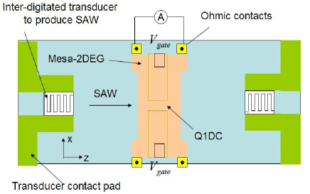
Figure 1: A schematic diagram of the MQD device Cunningham ; KataokaL ; Kataoka ; Robinson .

For simplicity, we assume that only one electron is captured into the MQD and then propagates along the narrow depleted Q1DC. The potential of the electron in a MQD could be effectively simplified as

$$V_{\rm eff}(z,t)=V_{\rm SAW}(z,t)+V_{\rm gate}(z),$$ (1)

where $V_{\rm SAW}(z,t)$ and $V_{\rm gate}(z)$ are the piezoelectric potential accompanying the SAW and the electrostatic potential defined by the surface split-gate, respectively. First, the thickness and width of the quantum dot (i.e., its sizes along the $y$- and $x$-direction) are all neglected, such that the electrostatic potential could be simply modeled as a strictly 1D potential GodfreyB ; Godfrey

$$V_{\rm gate}(z)=\frac{V_{0}}{\cosh^{2}(z/a)}.$$ (2)

Here, the $z$-axis is chosen along the channel which the SAW propagates through and the parameter $V_{0}$ determines the effective height of the potential barrier. The split-gate is operated well beyond the pinch off voltage in the absence of the SAW, so the energy $V_{0}$ could be greater than the electron Fermi energy in the 2DEG, and the edge of the depleted Q1DC is well away from the edge of the surface split-gate. The effective length of the Q1DC can be taken as $l_{\rm eff}=2a$, and it takes also approximately as long as the SAW wavelength $\lambda=1\mu$m. Consequently, we have $a=0.5~{}\mu$m. Next, by considering the screening effect of the metal gates on the SAW-induced electric potential, and neglecting the mechanical coupling between the semiconductor and the metal surface gate, all the changes in the components of the stress tensor, and the separation between split-gates, etc., Aǐzin $et~{}al$ Aizin showed that the piezoelectric potential $V_{\rm SAW}$ could be simplified to the form

$$V_{\rm SAW}=V_{S}\cos(kz-wt).$$ (3)

Here, $V_{S}$ is the amplitude of the SAW, and $k$ and $w$ are the frequency and wave number, respectively.

With the above potential the electronic levels of the electron trapped in the MQD can be determined by solving the instantaneous eigenvalue equation

$$\hat{H}_{0}(t)\rvert E_{n}(t)\rangle=E_{n}(t)\rvert\psi_{n}(t)\rangle,$$

$$\hat{H}_{0}(t)=-\frac{\hbar^{2}}{2m^{*}}\frac{d^{2}}{dz^{2}}+\frac{V_{0}}{\cosh^{2}(z/a)}+V_{S}\cos(kx-wt).$$ (4)

Here, $m^{*}=0.0067m_{e}$ is the effective mass of the electron in GaAs, and $V_{0}=\hbar^{2}/2m^{*}l_{0}^{2}$, $V_{S}=\gamma V_{0}$. The parameter $l_{0}=4\times 10^{-2}a$ is the effective width of the Q1DC, and $\gamma=0.5$ the ratio of the SAW potential amplitude to the height of the electrostatically-induced potential barrier in the Q1DC. The SAW velocity is $v=2981$m/s GodfreyB . By finite differential method we can numerically solve Eq. (4) and obtain the electronic levels in the MQD. Although the shape of the potential or the size of the quantum dot changes with the motion, the dot is still “big” enough to hold a few levels. Specifically, Fig. 2 shows the effective potential and its corresponding bound levels for the different times over the SAW period. Qualitatively, the dot could capture many electrons initially, but most of them will be escaped from the local well and returned to the source reservoir. In the present calculation, we consider the ideal condition wherein only one electron is initially captured by the MQD and held in where across the channel. One can see from Fig. 2 that, a few bound levels exist in the local potential of the quantum dot moving along the channel. The wave function and the corresponding probabilistic distributions of the electron residing in these levels are shown in Fig. 3. One can see that the electron in the third (blue-line) level or the higher ones could escape from the well. While, the probabilities of the electron in the lowest two levels, the ground and first excited ones, tunneling to the source reservoir is negligible. As a consequence, these two levels can be used to encode the desirable flying qubit, the unit of the moving quantum information.

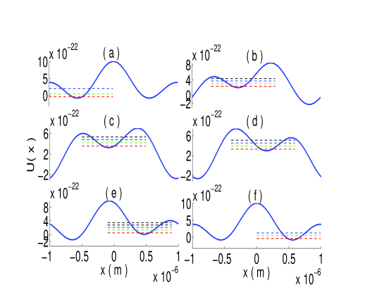
Figure 2: The effective potential and its allowed energy levels for $\gamma=0.5$ at various typical times: (a) $t=0$, (b) $t=0.1$ns, (c) $t=0.15$ns, (d) $t=0.2$ns, (e) $0.3\times 10^{-9}~{}s$, and (f) $t=T=0.34$ns. The blue solid line represent the effective potential and the colored dashed-lines show the allowed levels: red (ground state), green (the first exited state), blue (the second excited state), etc..

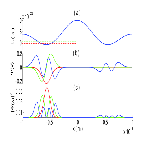
Figure 3: Wave functions of the lowest three levels and their relevant probabilistic distributions at certain time: (a) Potential and its allowed levels, (b) The eigenfunctions of the allowed levels and (c) the probabilistic distributions of the electron in the allowed-levels along the channel. Here, the red, green and blue lines denote the ground, the first excited and the second excited state, respectively.

We now show that the flying qubit defined above is sufficiently stationary, although the shape of the potential varies with the quantum dot moving along the channel. The adiabatic theorem asserts that, if the rate of the change of Hamiltonian is slow enough, the system will stay at an instantaneous eigenstate of the time-Hamiltonian. For the present case the adiabatic condition is expressed as

$$\beta=\left|\frac{\hbar\langle m\lvert\frac{\partial H_{0}(t)}{\partial t}\rvert n\rangle}{(E_{m}(t)-E_{n}(t))^{2}}\right|\ll 1,$$ (5)

where $E_{m}(t)-E_{n}(t)$ is the energy splitting between the state $\rvert m\rangle$ and $\rvert n\rangle$. Our numerical results show that, at certain time: $E_{0}=-3.57\times 10^{-23}~{}J,E_{1}=4.80\times 10^{-23}~{}J$ and consequently $\beta=0.0289$. This indicates that the adiabatic condition could be satisfied. Less value of the $\beta$-parameter is also possible by properly adjusting the relevant parameters. This means that the levels used above to encode the flying qubit is adiabatic. Thus, once the flying qubit is prepared at one of its logic states ($|0\rangle$ and $|1\rangle$), it always stays at that state until the specific driving is applied.

III Rabi oscillations between the levels of flying qubit

For realizing quantum computation, we need to first implement arbitrary rotations of the single-qubit. For the present flying qubit, this can be achieved by using the usual Rabi oscillations between the adiabatic states $\rvert 0\rangle$ and $\rvert 1\rangle$. Basically, these states should be kept as the pure ones. This can be realized by cooling the system to a sufficiently low temperature $T_{\rm temp}$, such that the condition $k_{B}T_{\rm temp}\ll\hbar\omega$ is satisfied. Here, $\omega=\omega_{1}-\omega_{0}$ is the electronic transition frequency of the flying qubit, and $k_{B}$ is Boltzmann constant. Experimentally KataokaL , the system can be worked approximately at the temperature $T_{\rm temp}=0.27~{}K$, yielding $k_{B}T_{\rm temp}=3.726\times 10^{-24}~{}J\ll\hbar\omega\sim 8.3667\times 10^{-23}~{}J$. Thus, the transitions between the qubit’s levels due to the thermal excitations can be safely neglected.

We now apply a resonant electric driving to the surface gates for implementing the desirable Rabi oscillations. Under such a driving the previous 1D-potential $V_{\rm gate}$, i.e., Eq. (2), is now changed as $V_{\rm gate}\rightarrow V^{\prime}_{\rm gate}=V_{\rm gate}+V_{e}\cos(\omega t)/\cosh^{2}(z/a)$. Consequently, the dynamics of the driven flying qubit is determined by the following time-dependent Schrödinger equation

$$i\hbar\frac{\partial\rvert\psi(t)\rangle}{\partial t}=(\hat{H}_{0}+\hat{H}^{\prime})\rvert\psi(t)\rangle.$$ (6)

Here,

$$\hat{H}^{\prime}=\frac{V_{e}\cos(\omega t)}{\cosh^{2}(z/a)},$$ (7)

describes the driving induced by the applied oscillating electric-field, which is perpendicular to the Q1DC and linearly polarized along the x-axis. Above, $V_{e}$ is a parameter depending on the power of the applied electric-filed. In our calculation, we choose it as $V_{e}=0.1V_{S}$ for simplicity. Generally, the wave function of the driven flying qubit can be written as

$$\rvert\psi(t)\rangle=C_{0}\rvert 0\rangle+C_{1}\rvert 1\rangle,$$ (8)

with $C_{0}$ and $C_{1}$ being the probability-amplitudes of finding the electron in the states $\rvert 0\rangle$ and $\rvert 1\rangle$, respectively.

From Eqs. (6-8), the equations of motion for the amplitudes $C_{0}$ and $C_{1}$ can be derived as

$$\frac{\partial C_{0}}{\partial t}=-i\omega_{0}C_{0}-iC_{0}D_{00}\cos{(\omega t)}-iC_{1}D_{01}\cos(\omega t),$$ (9)

and

$$\frac{\partial C_{1}}{\partial t}=-i\omega_{1}C_{1}-iC_{1}D_{11}\cos{(\omega t)}-iC_{0}D_{10}\cos(\omega t),$$ (10)

with $D_{ij}=V_{e}/[\hbar\langle i|\cosh^{2}(z/a)|j\rangle],\,i,j=0,1$. The above equations can be exactly solved by numerical method. Then, the time-dependent probabilities of the electron being in the states $\lvert 0\rangle$ and $\lvert 1\rangle$ can be obtained as $\lvert C_{0}(t)\rvert^{2}$ and $\lvert C_{1}(t)\rvert^{2}$, respectively. Certainly, the relation

$$\lvert C_{0}(t)\rvert^{2}+\lvert C_{1}(t)\rvert^{2}=1,$$ (11)

is always satisfied. With the initial condition $|\psi(0)\rangle=|0\rangle$ we plot the time-dependent $|C_{1}(t)|^{2}$ in Fig. 4. It is seen really that the population in one of the logic state of the flying reveals a obviously oscillating behavior with a period: $\tau\sim 0.32$ ns for the parameters selected above. This time-interval is sufficiently-long for the MQD across the Q1DC demonstrated in the experiment. The time interval for a quantum dot across the channel is estimated as $\sim 0.34~{}ns$. Thus, Rabi oscillations can be really utilized to realize the desirable single-qubit operations.

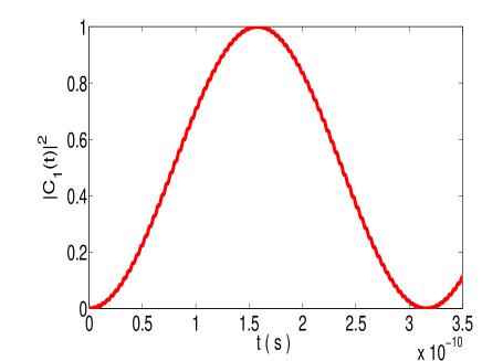
Figure 4: Rabi oscillation of the population in flying qubit’s level $|1\rangle$. The oscillation period shown here is about $0.32$ ns.

IV Coupling the separated moving quantum dots for two-flying-qubit operations

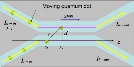
Figure 5: The schematic diagram to implement controllable couplings between two flying-qubits. Two MQDs passage along the the upper- and lower Q1DCs, respectively and the coupling between them is realized by the Coulomb interaction of the inside electrons.

We now discuss how to implement an universal gate, i.e., the two-qubit operation, with the MQDs. A simple way to achieve such a task is by utilizing the Coulomb interaction between the electrons in the nearest-neighbour interaction MQDs. To do this, let us consider the situation schematically shown in Fig. 5, wherein two MQDs driven by two SAWs pass across two Q1DCs, the upper- and lower ones. Suppose that the tunneling between them is negligible and only the Coulomb interaction between them is important. First, the Coulomb force between the electrons in these two MQDs can be expressed as

$$F_{\rm int}(z_{u},z_{l})=\frac{e^{2}}{4\pi\varepsilon_{0}}\frac{(z_{l}-z_{u})}{[d^{2}+(z_{l}-z_{u})^{2}]^{3/2}},$$ (12)

with $z_{u}$ and $z_{l}$ being their coordinates along the channels (the indices $u$ and $l$ refer to the upper and lower channels, respectively) and $d$ the distance between the two Q1DCs. Since the motions of the electrons are always along the Q1DCs, the vertical force of the Coulomb interaction can be ignored and thus only the horizontal force along the z-axis is taken account into. Second, the potential related to above force can be written as

$$\begin{array}[]{l}V_{\rm int}(z)=\frac{1}{4\pi\varepsilon_{0}}\int_{0}^{z}\frac{e^{2}zdz}{(d^{2}+z^{2})^{3/2}}\\ \\ \,\,\,\,\,\,\,\,\,\,\,\,\,\,\,\,\,\,\,=-\frac{1}{4\pi\varepsilon_{0}}\frac{e^{2}}{d}\left\{\frac{1}{[1+(z/d)^{2}]^{1/2}}-1\right\},\end{array}$$ (13)

where $z=z_{l}-z_{u}$. By using the usual Taylor expansion and ignoring the high-order terms under the condition $d\gg z$, the above Coulomb potential reduces to

$$V_{\rm int}(z)=\frac{e^{2}}{8\pi\varepsilon_{0}d^{3}}z^{2}=\frac{e^{2}}{8\pi\varepsilon_{0}d^{3}}\left(z_{u}^{2}+z_{l}^{2}-2z_{u}z_{l}\right).$$ (14)

Thirdly, the Hamiltonian describing the dynamics of the two-coupling MQDs reads

$$\hat{H}_{h} =\hat{H}_{t}+V_{\rm int}(z),$$ (15)

with

$$\begin{array}[]{l}\hat{H}_{t}=\sum_{j=u,l}\left[-\frac{\hbar^{2}}{2m_{j}^{*}}\frac{d^{2}}{dz_{j}^{2}}+\frac{V_{0}^{j}}{\cosh^{2}(z_{j}/a)}+V_{S}^{j}\cos(kz_{j}-\omega t)\right]\\ \\ \,\,\,\,\,\,\,\,\,=\sum_{j=u,l}\frac{\hbar\omega_{j}}{2}\hat{\sigma}_{j}^{z},\end{array}$$ (16)

and $\hat{\sigma}_{j}^{z}=\rvert 1_{j}\rangle\langle 1_{j}\lvert-\rvert 0_{j}\rangle\langle 0_{j}\lvert$, $\omega_{j}=(E_{1}^{j}-E_{0}^{j})/\hbar$.

In the qubit representation, the position operators $\hat{z}_{j}$, $\hat{z}_{j}^{2}$ and $\hat{z}_{j}\hat{z}_{k}$ (where $j,k=u,l$ and $j\neq k$) can be expressed as

$$\begin{array}[]{l}\hat{z}_{j}=\frac{1}{2}(z_{j}^{11}-z_{j}^{00})\hat{\sigma}_{j}^{z}+z_{j}^{01}\hat{\sigma}_{j}^{x},\\ \\ \hat{z}_{j}^{2}=\frac{1}{2}(z_{j}^{11}+z_{j}^{00})(z_{j}^{11}-z_{j}^{00})\hat{\sigma}_{j}^{z}\\ \\ \,\,\,\,\,\,\,\,\,\,\,\,+(z_{j}^{00}+z_{j}^{11})z_{j}^{01}\hat{\sigma}_{j}^{x},\end{array}$$ (17)

and

$$\begin{array}[]{l}\hat{z}_{j}\hat{z}_{k}=\frac{1}{4}(z_{k}^{11}+z_{k}^{00})(z_{j}^{11}-z_{j}^{00})\hat{\sigma_{j}^{z}}+z_{j}^{01}z_{k}^{01}\hat{\sigma}_{j}^{x}\hat{\sigma}_{k}^{x}\\ \\ \,\,\,\,\,\,\,\,\,\,\,\,\,\,\,\,\,\,+\frac{1}{4}(z_{j}^{11}+z_{j}^{00})(z_{k}^{11}-z_{k}^{00})\hat{\sigma_{k}^{z}}\\ \\ \,\,\,\,\,\,\,\,\,\,\,\,\,\,\,\,\,\,+\frac{1}{2}(z_{k}^{00}+z_{k}^{11})z_{j}^{01}\hat{\sigma_{j}^{x}}+\frac{1}{2}(z_{j}^{00}+z_{j}^{11})z_{k}^{01}\hat{\sigma_{k}^{x}}\\ \\ \,\,\,\,\,\,\,\,\,\,\,\,\,\,\,\,\,\,+\frac{1}{4}(z_{j}^{11}-z_{j}^{00})(z_{k}^{11}-z_{k}^{00})\hat{\sigma_{j}^{z}}\hat{\sigma_{k}^{z}}\\ \\ \,\,\,\,\,\,\,\,\,\,\,\,\,\,\,\,\,\,+\frac{1}{2}(z_{j}^{11}-z_{j}^{00})z_{k}^{01}\hat{\sigma}_{j}^{z}\hat{\sigma}_{k}^{x}+\frac{1}{2}(z_{k}^{11}-z_{k}^{00})z_{j}^{01}\hat{\sigma}_{j}^{z}\hat{\sigma}_{k}^{x},\end{array}$$ (18)

respectively. Above, $\hat{\sigma}_{j}^{x}=\hat{\sigma}_{j}^{+}+\hat{\sigma}_{j}^{-}$ with $\hat{\sigma}_{j}^{+}=\rvert 1_{j}\rangle\langle 0_{j}\lvert$ and $\hat{\sigma}_{j}^{-}=\rvert 0_{j}\rangle\langle 1_{j}\lvert$; $z_{j}^{11}$, $z_{j}^{00}$ and $z_{j}^{01}$ are the matrix elements $\langle 1_{j}\lvert z_{j}\rvert 1_{j}\rangle$, $\langle 0_{j}\lvert z_{j}\rvert 0_{j}\rangle$, and $\langle 1_{j}\lvert z_{j}\rvert 0_{j}\rangle$, respectively. As a consequence, the above Coulomb potential $V_{\rm int}(z)$ can be rewritten as

$$\begin{array}[]{l}\hat{V}_{\rm int}=C_{u}^{z}\hat{\sigma}_{u}^{z}+C_{l}^{z}\hat{\sigma}_{l}^{z}+C_{u}^{x}\hat{\sigma}_{u}^{x}+C_{l}^{x}\hat{\sigma}_{l}^{x}+C_{ul}^{zz}\hat{\sigma}_{u}^{z}\hat{\sigma}_{l}^{z}\\ \\ \,\,\,\,\,\,\,\,\,\,\,\,\,\,\,\,+C_{ul}^{xx}\hat{\sigma}_{u}^{x}\hat{\sigma}_{l}^{x}+C_{ul}^{zx}\hat{\sigma}_{u}^{z}\hat{\sigma}_{l}^{x}+C_{ul}^{xz}\hat{\sigma}_{u}^{x}\hat{\sigma}_{l}^{z},\end{array}$$ (19)

with

$$\left\{\begin{array}[]{l}C_{u}^{z}=\frac{e^{2}}{16\pi\varepsilon_{0}d^{3}}(z_{u}^{00}+z_{u}^{11}-z_{l}^{00}-z_{l}^{11})(z_{u}^{11}-z_{u}^{00}),\\ \\ C_{l}^{z}=\frac{e^{2}}{16\pi\varepsilon_{0}d^{3}}(z_{l}^{00}+z_{l}^{11}-z_{u}^{00}-z_{u}^{11})(z_{l}^{11}-z_{l}^{00}),\\ \\ C_{u}^{x}=\frac{e^{2}}{8\pi\varepsilon_{0}d^{3}}(z_{u}^{00}+z_{u}^{11}-z_{l}^{00}-z_{l}^{11})z_{u}^{01},\\ \\ C_{l}^{x}=\frac{e^{2}}{8\pi\varepsilon_{0}d^{3}}(z_{l}^{00}+z_{l}^{11}-z_{u}^{00}-z_{u}^{11})z_{l}^{01},\end{array}\right.$$ (27)

and

$$\left\{\begin{array}[]{l}C_{ul}^{zz}=\frac{-e^{2}}{16\pi\varepsilon_{0}d^{3}}(z_{u}^{11}-z_{u}^{00})(z_{l}^{11}-z_{l}^{00}),\\ \\ C_{ul}^{xx}=\frac{-e^{2}}{4\pi\varepsilon_{0}d^{3}}z_{u}^{01}z_{l}^{01},\\ \\ C_{ul}^{zx}=\frac{-e^{2}}{8\pi\varepsilon_{0}d^{3}}(z_{u}^{11}-z_{u}^{00})z_{l}^{01},\\ \\ C_{ul}^{xz}=\frac{-e^{2}}{8\pi\varepsilon_{0}d^{3}}(z_{l}^{11}-z_{l}^{00})z_{u}^{01}.\end{array}\right.$$ (35)

In the interaction picture defined by the unitary $\hat{U}_{0}(t)=\exp{[(-i/\hbar)t\sum_{j=u,l}\lambda_{j}\hat{\sigma}_{j}^{z}]}$ with $\lambda_{j}=\hbar\omega_{j}/2+C_{j}^{z}$, the Hamiltonian of the system reduces to

$$\begin{array}[]{l}\hat{H}_{I}=C_{ul}^{zz}\hat{\sigma}_{u}^{z}\hat{\sigma}_{l}^{z}+\sum_{j=u,l}C_{j}^{x}\left(e^{2it\lambda_{j}/\hbar}\hat{\sigma}_{j}^{+}+e^{-2it\lambda_{j}/\hbar}\hat{\sigma}_{j}^{-}\right)\\ \\ \,\,\,\,\,\,\,\,\,\,\,\,\,\,\,\,+C_{ul}^{xx}[e^{2it(\lambda_{u}+\lambda_{l})/\hbar}\hat{\sigma}_{u}^{+}\hat{\sigma}_{l}^{+}+e^{2it(\lambda_{u}-\lambda_{l})/\hbar}\hat{\sigma}_{u}^{+}\hat{\sigma}_{l}^{-}\\ \\ \,\,\,\,\,\,\,\,\,\,\,\,\,\,\,\,+e^{-2it(\lambda_{u}-\lambda_{l})/\hbar}\hat{\sigma}_{u}^{-}\hat{\sigma}_{l}^{+}+e^{-2it(\lambda_{u}+\lambda_{l})/\hbar}\hat{\sigma}_{u}^{-}\hat{\sigma}_{l}^{-}]\\ \\ \,\,\,\,\,\,\,\,\,\,\,\,\,\,\,\,+C_{ul}^{zx}\left(e^{2it\lambda_{l}/\hbar}\hat{\sigma}_{u}^{z}\hat{\sigma}_{l}^{+}+e^{-2it\lambda_{l}/\hbar}\hat{\sigma}_{u}^{z}\hat{\sigma}_{l}^{-}\right)\\ \\ \,\,\,\,\,\,\,\,\,\,\,\,\,\,\,\,+C_{ul}^{xz}\left(e^{2it\lambda_{u}/\hbar}\hat{\sigma}_{u}^{+}\hat{\sigma}_{l}^{z}+e^{-2it\lambda_{u}/\hbar}\hat{\sigma}_{u}^{-}\hat{\sigma}_{l}^{z}\right).\end{array}$$ (36)

Consequently, under the usual rotating-wave approximation, we have

$$\overline{H}_{I}=C_{ul}^{xx}(\hat{\sigma}_{u}^{+}\hat{\sigma}_{l}^{-}+\hat{\sigma}_{u}^{-}\hat{\sigma}_{l}^{+}).$$ (37)

During this derivation, the significantly-small quantities $C_{ul}^{zz}\ll C_{ul}^{xx}$ has been omitted, and we have also assumed that $\lambda_{u}=\lambda_{l}$. Typically, for the experimental parameters: $z=2.981\times 10^{-2}\mu$m, we have $z_{u}^{00}=-5.6186\times 10^{-1}\mu\text{m},\,z_{u}^{11}=-5.6975\times 10^{-1}\mu\text{m},\,z_{u}^{01}=z_{u}^{10}=-5.6431\times 10^{-2}\mu\text{m}$; $z_{l}^{00}=-5.3594\times 10^{-1}\mu\text{m},\,z_{l}^{11}=-5.4418\times 10^{-1}\mu\text{m},\,z_{l}^{01}=z_{l}^{10}=-5.6607\times 10^{-2}\mu\text{m}$, and thus $C_{ul}^{zz}/C_{ul}^{xx}=1.3\times 10^{-3}\ll 1$.

Finally, the above Hamiltonian yield the following two qubit evolution (in the representation with the basis$\{\rvert 11\rangle,\rvert 10\rangle,\rvert 01\rangle,\rvert 00\rangle\}$

$$\hat{U}=e^{-i\hat{H}_{I}t/\hbar}=\left(\begin{array}[]{cccc}1&0&0&0\\ 0&\cos{\xi}&-i\sin{\xi}&0\\ 0&-i\sin{\xi}&\cos{\xi}&0\\ 0&0&0&1\end{array}\right),\,\,\xi=tC_{ul}^{xx}/\hbar.$$ (42)

This is the typical two-qubit i-SWAP gate. With such an universial gate, assisted by arbitrary rotations of single qubits, any quantum computing network could be constructed Lloyd .

V Discussions and conclusions

Readout of the qubits is another crucial tasks in quantum computing. In Barnes et al’s scheme Barnes , the flying qubit is encoded by the spin-states of the electrons in the MQDs and its readout is implemented by using the usually magnetic Stern-Gerlach effect. In our proposal the flying qubit is encoded by the lowest two levels of the electron in the moving trapped potential. These levels are theoretically steady but still exist weak tunnelings. Thus, by detecting the tunnelings of the moving electron from the trapped potential, one can achieve the qubit readouts. This is because that the tunneling rates of electron in either the state $|0\rangle$ or the state $|1\rangle$ should be different and thus could be distinguished individually. In fact, these tunneling-measurements have been realized in the recent experiment KataokaL . There, another channel is introduced to detect the tunnelings of the electrons in the MQDs across the computational channels. Physically, the flying electron in the state $|1\rangle$ should yield significantly-high probability of tunneling to the detecting channel, and thus decrease the current $I_{\rm top}$ flowing along the computational channel. While, if the flying electron in the ground level $|0\rangle$, then the probability of tunneling out should be obviously small and thus $I_{\rm top}$ should be almost unchanged. Stronger tunnelings are also possible, if the flying qubit is excited for leakage. This can be achieved by applying a resonant pulse to excite the electron staying at the computational basis $|0\rangle$ (or $|1\rangle$) to the higher level (e.g., the state $|2\rangle$) with significantly-bigger tunneling-probabilities pepper07 . By this way, flying qubit staying at $|0\rangle$ or $|1\rangle$ could be more robustly detected.

Another challenge for realizing our proposal is how to hold only one electron in a MQD across the computational channel. Initially, many electrons can be captured by the SAWs from the source region of 2DEG; the number of electrons residing in the minima of SAWs depend on the size of the formed quantum dot. Note that the static potential generated by the split-gate is fixed, but the depth and the curvature of the MQD vary with the time during the MQD moving along the channel. When the size of the dot becomes smaller, electrons captured from the source are ejected from the dot and let a few ones be still trapped by the potential. By suitably controlling the relevant parameters, e.g., the power of the SAW and the split-gate voltage, only one electron could reside in a MQD for realizing the desirable flying qubit. Finally, as in all the other solid-state quantum computing candidates, decoherence in the present flying qubit is also an open problem and would be discussed in future.

In summary, we have put forward an approach to implementing quantum computation with the energy levels of the electrons trapped in the MQDs. The idea involves the capture of electrons from a 2DEG by the SAWs to form the potentials for trapping a single electron. Each SAW may capture many electrons from the 2DEG source, but we can make only one electron reside in the minimum of the SAW by tuning the surface split-gate to change the barrier height, that forces the excessive electrons to tunnel out from the quantum dot. By numerical method, we have known that few adiabatic levels of each electron could be formed in a MQD, and the lowest two ones are utilized to encode a flying qubit. We have shown how to implement the Rabi oscillations with the flying qubit for performing single-qubit operation. A two-qubit gate, i.e., i-SWAP gate, has also be constructed by using the Coulomb interaction of the electrons in different MQDs across the nearest-neighbor computational channels. In principle, our proposal can be extended to the system including $N$ qubits by integrating an array of $N$ Q1DCs.

References

- (1) S. Lloyd, Science 261, 5128 (1993).
- (2) P. W. Shor, Proceedings of the 35th Annual Symposium on Foundations of Computer Science (IEEE Computer Press,Los Alamitos, 1994), p. 124.
- (3) A. S. Parkins, P. Marte and P. Zoller, Phys. Rev. Lett. 71, 3095 (1993).
- (4) T. Pellizzari, S. A. Gardiner, J. I. Cirac and P. Zoller, Phys. Rev. Lett. 45, 3788 (1995).
- (5) See, e.g., J. I. Cirac and P. Zoller, Phys. Rev. Lett. 74, 4091 (1995); L. F. Wei, S. Y. Liu, and X. L. Lei, Phys. Rev. A 65, 062316 (2002).
- (6) N. A. Gershenfeld and I. L. Chuang, Science 275, 350-356 (1997).
- (7) D. Bouwmeester, J. W. Pan, M. Daniell, H. Weinfurter and A. Zeilinger, Phys. Rev. Lett. 82, 1345 (1999).
- (8) Y. H. Kim, S. P. Kulik, M. V. Cekhova, W. P. Grice and Y. Shih, Phys. Rev. A 67, 010301 (2003).
- (9) D. Loss and D. P. DiVincenzo, Phys. Rev. A 57, 120 (1998).
- (10) K. R. Brown, D. A. Lidar and K. B. Whaley, Phys. Rev. A 65, 012307 (2001).
- (11) See, e.g., Y. Makhlin, G. Schön, and A. Shnirman, Rev. Mod. Phys. 73, 357 (2001); L. F. Wei, Yu-xi Liu, and Franco Nori, Phys. Rev. B 71, 134506 (2005).
- (12) J. M. Shilton, V. I. Talyanskii, M. Pepper, D. A. Ritchie, J. E. F. Frost, C. J. V. Ford, C. G. Smith and G. A. C. Jones, J. Phys. Condens. Matter 8, L531 (1996).
- (13) V. I. Talyanskii, J. M. Shiltion, M. Pepper, C. G. Smith, C. J. B. Ford, E. H. Linfield, D. A. Ritchie, and G. A. C. Jones, Phys. Rev. B 56, 15180 (1997).
- (14) C. H. W. Barnes, J. M. Shilton, and A. M. Robinson, Phys. Rev. B 62, 8410 (2000).
- (15) S. Furuta, C. H. W. Barnes, and C. J. L. Doran, Phys. Rev. B 70, 205320 (2004).
- (16) R. Rodriquez, D. K. L. Oi, M. Kataoka, C. H. W. Barnes, T. Ohshima and A. K. Ekert, Phys. Rev. B 72, 085329 (2005).
- (17) P. Bordone, A. Bertoni, MRosini, S. Reggiani and C. Jacoboni, Semicond. Sci. Technol. 19, S412 (2004).
- (18) M. Kataoka, M. R. Astley, A. L. Thorn, D. K. L. Oi, C. H. W. Barnes, C. J. B. Ford, D. Anderson, G. A. C. Jones, I. Farrer, D. A. Ritchie, and M. Pepper, Phys. Rev. Lett. 102, 156801 (2009).
- (19) J. Cunningham, V. I. Talyanskii, J. M. Shilton, M. Pepper, M. Y. Simmons and D. A. Ritchie, Phys. Rev. B 60, 4850 (1999).
- (20) M. Kataoka, R. J. Schneble, A. L. Thorn, C. H. W. Branes, X. J. V. Ford, D. Anderson, G. A. C. Jones, I. Farrer, D. A. Ritchie, and M. Pepper, Phys. Rev. Lett. 98, 046801 (2007).
- (21) A. M. Robinson and C. H. W. Barnes, Phys. Rev. B 63, 165418 (2001).
- (22) G. Gumbs, G. R. Aǐzin and M. Pepper, Phys. Rev. B 60, 13954 (1999).
- (23) G. Gumbs and Y. Abranyos, Phys. Rev. A 70, 050302 (2004).
- (24) G. R. Aǐzin, G. Gumbs, and M. Pepper, Phys. Rev. B 58, 10589 (1998).
- (25) M. R. Astley, M. Kataoka, C. J. B. Ford, C. H. W. Barnes, D. Anderson, G. A. C. Jones, I. Farrer, D. A. Ritchie, and M. Pepper Phys. Rev. Lett. 99, 156802 (2007).