A Generalized Least Squares Matrix Decomposition

Abstract

Variables in many massive high-dimensional data sets are structured, arising for example from measurements on a regular grid as in imaging and time series or from spatial-temporal measurements as in climate studies. Classical multivariate techniques ignore these structural relationships often resulting in poor performance. We propose a generalization of the singular value decomposition (SVD) and principal components analysis (PCA) that is appropriate for massive data sets with structured variables or known two-way dependencies. By finding the best low rank approximation of the data with respect to a transposable quadratic norm, our decomposition, entitled the Generalized least squares Matrix Decomposition (GMD), directly accounts for structural relationships. As many variables in high-dimensional settings are often irrelevant or noisy, we also regularize our matrix decomposition by adding two-way penalties to encourage sparsity or smoothness. We develop fast computational algorithms using our methods to perform generalized PCA (GPCA), sparse GPCA, and functional GPCA on massive data sets. Through simulations and a whole brain functional MRI example we demonstrate the utility of our methodology for dimension reduction, signal recovery, and feature selection with high-dimensional structured data.
Keywords: matrix decomposition, singular value decomposition, principal components analysis, sparse PCA, functional PCA, structured data, neuroimaging.

1 Introduction

Principal components analysis (PCA), and the singular value decomposition (SVD) upon which it is based, form the foundation of much of classical multivariate analysis. It is well known, however, that with both high-dimensional data and functional data, traditional PCA can perform poorly (Silverman, 1996; Jolliffe et al., 2003; Johnstone and Lu, 2004). Methods enforcing sparsity or smoothness on the matrix factors, such as sparse or functional PCA, have been shown to consistently recover the factors in these settings (Silverman, 1996; Johnstone and Lu, 2004). Recently, these techniques have been extended to regularize both the row and column factors of a matrix (Huang et al., 2009; Witten et al., 2009; Lee et al., 2010). All of these methods, however, can fail to capture relevant aspects of structured high-dimensional data. In this paper, we propose a general and flexible framework for PCA that can directly account for structural dependencies and incorporate two-way regularization for exploratory analysis of massive structured data sets.

Examples of high-dimensional structured data in which classical PCA performs poorly abound in areas of biomedical imaging, environmental studies, time series and longitudinal studies, and network data. Consider, for example, functional MRIs (fMRIs) which measure three-dimensional images of the brain over time with high spatial resolution. Each three-dimensional pixel, or voxel, in the image corresponds to a measure of the bold oxygenation level dependent (BOLD) response (hereafter referred to as “activation”), an indirect measure of neuronal activity at a particular location in the brain. Often these voxels are vectorized at each time point to form a high-dimensional matrix of voxels ($\approx$ 10,000 - 100,000) by time points ($\approx$ 100 - 10,000) to be analyzed by multivariate methods. Thus, this data exhibits strong spatial dependencies among the rows and strong temporal dependencies among the columns (Lindquist, 2008; Lazar, 2008). Multivariate analysis techniques are often applied to fMRI data to find regions of interest, or spatially contiguous groups of voxels exhibiting strong co-activation as well as the time courses associated with these regions of activity (Lindquist, 2008). Principal components analysis and the SVD, however, are rarely used for this purpose. Many have noted that the first several principal components of fMRI data appear to capture spatial and temporal dependencies in the noise rather than the patterns of brain activation in which neuroscientists are interested. Furthermore, subsequent principal components often exhibit a mixture of noise dependencies and brain activation such that the signal in the data remains unclear (Friston et al., 1999; Calhoun et al., 2001; Thirion and Faugeras, 2003; Viviani et al., 2005). This behavior of classical PCA is typical when it is applied to structured data with low signal compared to the noise dependencies induced by the data structure.

To understand the poor performance of the SVD and PCA is these settings, we examine the model mathematically. We observe data $\operatorname{\mathbf{Y}}\in\Re^{n\times p}$, for which standard PCA considers the following model: $\operatorname{\mathbf{Y}}=\operatorname{\mathbf{M}}+\operatorname{\mathbf{U}}\operatorname{\mathbf{D}}\operatorname{\mathbf{V}}^{T}+\operatorname{\mathbf{E}}$, where $\operatorname{\mathbf{M}}$ denotes a mean matrix, $\operatorname{\mathbf{D}}$ the singular values, $\operatorname{\mathbf{U}}$ and $\operatorname{\mathbf{V}}$ the left and right factors, respectively, and $\operatorname{\mathbf{E}}$ the noise matrix. Implicitly, SVD models assume that the elements of $\operatorname{\mathbf{E}}$ are independently and identically distributed, as the SVD is calculated by minimizing the Frobenius norm loss function: $||\operatorname{\mathbf{X}}-\operatorname{\mathbf{U}}\operatorname{\mathbf{D}}\operatorname{\mathbf{V}}^{T}||_{F}^{2}=\sum_{i=1}^{n}\sum_{j=1}^{p}(X_{ij}-\operatorname{\mathbf{u}}_{i}\operatorname{\mathbf{D}}\operatorname{\mathbf{v}}_{j}^{T})^{2}$, where $\operatorname{\mathbf{u}}_{i}$ is the $i^{th}$ column of $\operatorname{\mathbf{U}}$ and $\operatorname{\mathbf{v}}_{j}$ is analogous and $\operatorname{\mathbf{X}}$ denotes the centered data, $\operatorname{\mathbf{X}}=\operatorname{\mathbf{Y}}-\operatorname{\mathbf{M}}$. This sums of squares loss function weights errors associated with each matrix element equally and cross-product errors, between elements $X_{ij}$ and $X_{i^{\prime}j^{\prime}}$, for example, are ignored. It comes as no surprise then that the Frobenius norm loss and thus the SVD perform poorly with data exhibiting strong structural dependencies among the matrix elements. To permit unequal weighting of the matrix errors according to the data structure, we assume that the noise is structured: $\mathrm{vec}(\operatorname{\mathbf{E}})\sim(\mathbf{0},\operatorname{\mathbf{R}}^{-1}\otimes\operatorname{\mathbf{Q}}^{-1})$, or the covariance of the noise is separable and has a Kronecker product covariance (Gupta and Nagar, 1999). Our loss function, then changes from the Frobenius norm to a transposable quadratic norm that permits unequal weighting of the matrix error terms based on $\operatorname{\mathbf{Q}}$ and $\operatorname{\mathbf{R}}$: $||\operatorname{\mathbf{X}}-\operatorname{\mathbf{U}}\operatorname{\mathbf{D}}\operatorname{\mathbf{V}}^{T}||_{\operatorname{\mathbf{Q}},\operatorname{\mathbf{R}}}^{2}=\sum_{i=1}^{n}\sum_{j=1}^{p}\sum_{i^{\prime}=1}^{n}\sum_{j^{\prime}=1}^{p}\operatorname{\mathbf{Q}}_{ii^{\prime}}\operatorname{\mathbf{R}}_{jj^{\prime}}(X_{ij}-\operatorname{\mathbf{u}}_{i}\operatorname{\mathbf{D}}\operatorname{\mathbf{v}}_{j}^{T})(X_{i^{\prime}j^{\prime}}-\operatorname{\mathbf{u}}_{i^{\prime}}\operatorname{\mathbf{D}}\operatorname{\mathbf{v}}_{j^{\prime}}^{T})$. By finding the best low rank approximation of the data with respect to this transposable quadratic norm, we develop a decomposition that directly accounts for two-way structural dependencies in the data. This gives us a method, Generalized PCA, that extends PCA for applications to structured data.

While this paper was initially under review, previous work on unequal weighting of matrix elements in PCA via a row and column generalizing operators came to our attention (Escoufier, 1977). This so called, “duality approach to PCA” is known in the French multivariate community, but has perhaps not gained the popularity in the statistics literature that it deserves. Developed predominately in the 1970’s and 80’s for applications in ecological statistics, few texts on this were published in English (Escoufier, 1977; Tenenhaus and Young, 1985; Escoufier, 1987). Recently, a few works review these methods in relation to classical multivariate statistics (Escoufier, 2006; Purdom, 2007; Dray and Dufour, 2007; Holmes, 2008). While these works propose a mathematical framework for unequal weighting matrices in PCA, much more statistical and computational development is needed in order to directly apply these methods to high-dimensional structured data.

In this paper, we aim to develop a flexible mathematical framework for PCA that accounts for known structure and incorporates regularization in a manner that is computationally feasible for analysis of massive structured data sets. Our specific contributions include (1) a matrix decomposition that accounts for known two-way structure, (2) a framework for two-way regularization in PCA and in Generalized PCA, and (3) results and algorithms allowing one to compute (1) and (2) for ultra high-dimensional data. Specifically, beyond the previous work in this area reviewed by Holmes (2008), we provide results allowing for (i) general weighting matrices, (ii) computational approaches for high-dimensional data, and (iii) a framework for two-way regularization in the context of Generalized PCA. As our methods are flexible and general, they will enjoy wide applicability to a variety of structured data sets common in medical imaging, remote sensing, engineering, environmetrics, and networking.

The paper is organized as follows. In Sections 2.1 through 2.5, we develop the mathematical framework for our Generalized Least Squares Matrix Decomposition and resulting Generalized PCA. In these sections, we assume that the weighting matrices, or quadratic operators are fixed and known. Then, by discussing interpretations of our approach and relations to existing methodology, we present classes of quadratic operators in Section 2.6 that are appropriate for many structured data sets. As the focus of this paper is the statistical methodology for PCA with high-dimensional structured data, our intent here is to give the reader intuition on the quadratic operators and leave other aspects for future work. In Section  3, we propose a general framework for incorporating two-way regularization in PCA and Generalized PCA. We demonstrate how this framework leads to methods for Sparse and Functional Generalized PCA. In Section  4, we give results on both simulated data and real functional MRI data. We conclude, in Section  5, with a discussion of the assumptions, implications, and possible extensions of our work.

2 A Generalized Least Squares Matrix Decomposition

We present a generalization of the singular value decomposition (SVD) that incorporates known dependencies or structural information about the data. Our methods can be used to perform Generalized PCA for massive structured data sets.

2.1 GMD Problem

Here and for the remainder of the paper, we will assume that the data, $\operatorname{\mathbf{X}}$ has previously been centered. We begin by reviewing the SVD which can be written as $\operatorname{\mathbf{X}}=\operatorname{\mathbf{U}}\operatorname{\mathbf{D}}\operatorname{\mathbf{V}}^{T}$ with the data $\operatorname{\mathbf{X}}\in\Re^{n\times p}$, and where $\operatorname{\mathbf{U}}\in\Re^{n\times p}$ and $\operatorname{\mathbf{V}}\in\Re^{p\times p}$ are orthonormal and $\operatorname{\mathbf{D}}\in\Re^{p\times p}$ is diagonal with non-negative diagonal elements. Suppose one wishes to find the best low rank, $K<\mathrm{min}(n,p)$, approximation to the data. Recall that the SVD gives the best rank-$K$ approximation with respect to the Frobenius norm (Eckart and Young, 1936):

$$\operatorname*{\mathrm{minimize}}_{\operatorname{\mathbf{U}}:\mathrm{rank}(\operatorname{\mathbf{U}})=K,\operatorname{\mathbf{D}}:\operatorname{\mathbf{D}}\in\mathcal{D},\operatorname{\mathbf{V}}:\mathrm{rank}(\operatorname{\mathbf{V}})=K}\ \ ||\operatorname{\mathbf{X}}-\operatorname{\mathbf{U}}\operatorname{\mathbf{D}}\operatorname{\mathbf{V}}^{T}||_{F}^{2}$$

subject to $$\operatorname{\mathbf{U}}^{T}\operatorname{\mathbf{U}}=\operatorname{\mathbf{I}}_{(K)},\ \ \operatorname{\mathbf{V}}^{T}\operatorname{\mathbf{V}}=\operatorname{\mathbf{I}}_{(K)}\ \ \&\ \ \mathrm{diag}(\operatorname{\mathbf{D}})\geq 0.$$ (1)

Here, $\mathcal{D}$ is the class of diagonal matrices. The solution is given by the first $K$ singular vectors and singular values of $\operatorname{\mathbf{X}}$.

The Frobenius norm weights all errors equally in the loss function. We seek a generalization of the SVD that allows for unequal weighting of the errors to account for structure or known dependencies in the data. To this end, we introduce a loss function given by a transposable quadratic norm, the $\operatorname{\mathbf{Q}},\operatorname{\mathbf{R}}$-norm, defined as follows:

Definition 1

Let $\operatorname{\mathbf{Q}}\in\Re^{n\times n}$ and $\operatorname{\mathbf{R}}\in\Re^{p\times p}$ be positive semi-definite matrices, $\operatorname{\mathbf{Q}},\operatorname{\mathbf{R}}\succeq 0$. Then the $\operatorname{\mathbf{Q}},\operatorname{\mathbf{R}}$-norm (or semi-norm) is defined as $||\operatorname{\mathbf{X}}||_{\operatorname{\mathbf{Q}},\operatorname{\mathbf{R}}}=\sqrt{\mathrm{tr}(\operatorname{\mathbf{Q}}\operatorname{\mathbf{X}}\operatorname{\mathbf{R}}\operatorname{\mathbf{X}}^{T})}$.

We note that if $\operatorname{\mathbf{Q}}$ and $\operatorname{\mathbf{R}}$ are both positive definite, $\operatorname{\mathbf{Q}},\operatorname{\mathbf{R}}\succ 0$, then the $\operatorname{\mathbf{Q}},\operatorname{\mathbf{R}}$-norm is a proper matrix norm. If $\operatorname{\mathbf{Q}}$ or $\operatorname{\mathbf{R}}$ are positive semi-definite, then it is a semi-norm, meaning that for $\operatorname{\mathbf{X}}\neq 0$, $||\operatorname{\mathbf{X}}||_{\operatorname{\mathbf{Q}},\operatorname{\mathbf{R}}}=0$ if $\operatorname{\mathbf{X}}\in null(\operatorname{\mathbf{Q}})$ or if $\operatorname{\mathbf{X}}^{T}\in null(\operatorname{\mathbf{R}})$. We call the $\operatorname{\mathbf{Q}},\operatorname{\mathbf{R}}$-norm a transposable quadratic norm, as it right and left multiplies $\operatorname{\mathbf{X}}$ and is thus an extension of the quadratic norm, or “norm induced by an inner product space” (Boyd and Vandenberghe, 2004; Horn and Johnson, 1985). Note that $||\operatorname{\mathbf{X}}||_{\operatorname{\mathbf{Q}}}\triangleq||\operatorname{\mathbf{X}}||_{\operatorname{\mathbf{Q}},\mathbf{I}}$ and $||\operatorname{\mathbf{X}}^{T}||_{\operatorname{\mathbf{R}}}\triangleq||\operatorname{\mathbf{X}}^{T}||_{\operatorname{\mathbf{R}},\mathbf{I}}$ are then quadratic norms.

The GMD is then taken to be the best rank-$K$ approximation to the data with respect to the $\operatorname{\mathbf{Q}},\operatorname{\mathbf{R}}$-norm:

$$\operatorname*{\mathrm{minimize}}_{\operatorname{\mathbf{U}}:\mathrm{rank}(\operatorname{\mathbf{U}})=K,\operatorname{\mathbf{D}}:\operatorname{\mathbf{D}}\in\mathcal{D},\operatorname{\mathbf{V}}:\mathrm{rank}(\operatorname{\mathbf{V}})=K}\hskip 11.38109pt ||\operatorname{\mathbf{X}}-\operatorname{\mathbf{U}}\operatorname{\mathbf{D}}\operatorname{\mathbf{V}}^{T}||_{\operatorname{\mathbf{Q}},\operatorname{\mathbf{R}}}^{2}$$

subject to $$\operatorname{\mathbf{U}}^{T}\operatorname{\mathbf{Q}}\operatorname{\mathbf{U}}=\operatorname{\mathbf{I}}_{(K)},\ \ \operatorname{\mathbf{V}}^{T}\operatorname{\mathbf{R}}\operatorname{\mathbf{V}}=\operatorname{\mathbf{I}}_{(K)}\ \ \&\ \ \mathrm{diag}(\operatorname{\mathbf{D}})\geq 0.$$ (2)

So we do not confuse the elements of the GMD with that of the SVD, we call $\operatorname{\mathbf{U}}$ and $\operatorname{\mathbf{V}}$ the left and right GMD factors respectively, and the diagonal elements of $\operatorname{\mathbf{D}}$, the GMD values. The matrices $\operatorname{\mathbf{Q}}$ and $\operatorname{\mathbf{R}}$ are called the left and right quadratic operators of the GMD respectively. Notice that the left and right GMD factors are constrained to be orthogonal in the inner product space induced by the $\operatorname{\mathbf{Q}}$-norm and $\operatorname{\mathbf{R}}$-norm respectively. Since the Frobenius norm is a special case of the $\operatorname{\mathbf{Q}},\operatorname{\mathbf{R}}$-norm, the GMD is in fact a generalization of the SVD.

We pause to motivate the rationale for finding a matrix decomposition with respect to the $\operatorname{\mathbf{Q}},\operatorname{\mathbf{R}}$-norm. Consider a matrix-variate Gaussian matrix, $\operatorname{\mathbf{X}}\sim N_{n,p}(\operatorname{\mathbf{U}}\operatorname{\mathbf{D}}\operatorname{\mathbf{V}}^{T},\operatorname{\mathbf{Q}}^{-1},\operatorname{\mathbf{R}}^{-1})$, or $\mathrm{vec}(\operatorname{\mathbf{X}})\sim N(\mathrm{vec}(\operatorname{\mathbf{U}}\operatorname{\mathbf{D}}\operatorname{\mathbf{V}}^{T}),\operatorname{\mathbf{R}}^{-1}\otimes\operatorname{\mathbf{Q}}^{-1})$ in terms of the familiar multivariate normal. The normal log-likelihood can be written as:

$$\ell(\operatorname{\mathbf{X}}|\operatorname{\mathbf{Q}}^{-1},\operatorname{\mathbf{R}}^{-1}) \propto\mathrm{tr}\left(\operatorname{\mathbf{Q}}(\operatorname{\mathbf{X}}-\operatorname{\mathbf{U}}\operatorname{\mathbf{D}}\operatorname{\mathbf{V}}^{T})\operatorname{\mathbf{R}}(\operatorname{\mathbf{X}}-\operatorname{\mathbf{U}}\operatorname{\mathbf{D}}\operatorname{\mathbf{V}}^{T})^{T}\right)=||\operatorname{\mathbf{X}}-\operatorname{\mathbf{U}}\operatorname{\mathbf{D}}\operatorname{\mathbf{V}}^{T}||_{\operatorname{\mathbf{Q}},\operatorname{\mathbf{R}}}^{2}.$$

Thus, as the Frobenius norm loss of the SVD is proportional to the log-likelihood of the spherical Gaussian with mean $\operatorname{\mathbf{U}}\operatorname{\mathbf{D}}\operatorname{\mathbf{V}}^{T}$, the $\operatorname{\mathbf{Q}},\operatorname{\mathbf{R}}$-norm loss is proportional to the log-likelihood of the matrix-variate Gaussian with mean $\operatorname{\mathbf{U}}\operatorname{\mathbf{D}}\operatorname{\mathbf{V}}^{T}$, row covariance $\operatorname{\mathbf{Q}}^{-1}$, and column covariance $\operatorname{\mathbf{R}}^{-1}$. In general, using the $\operatorname{\mathbf{Q}},\operatorname{\mathbf{R}}$-norm loss assumes that the covariance of the data arises from the Kronecker product between the row and column covariances, or that the covariance structure is separable. Several statistical tests exist to check these assumptions with real data (Mitchell et al., 2006; Li et al., 2008). Hence, if the dependence structure of the data is known, taking the quadratic operators to be the inverse covariance or precision matrices directly accounts for two-way dependencies in the data. We assume that $\operatorname{\mathbf{Q}}$ and $\operatorname{\mathbf{R}}$ are known in the development of the GMD and discuss possible choices for these with structured data in Section 2.5.

2.2 GMD Solution

The GMD solution, $\hat{\operatorname{\mathbf{X}}}=\operatorname{\mathbf{U}}^{*}\operatorname{\mathbf{D}}^{*}(\operatorname{\mathbf{V}}^{*})^{T}$, is comprised of $\operatorname{\mathbf{U}}^{*},\operatorname{\mathbf{D}}^{*}$ and $\operatorname{\mathbf{V}}^{*}$, the optimal points minimizing the GMD problem (2.1). The following result states that the GMD solution is an SVD of an altered data matrix.

Theorem 1

Suppose $\mathrm{rank}(\operatorname{\mathbf{Q}})=l$ and $\mathrm{rank}(\operatorname{\mathbf{R}})=m$. Decompose $\operatorname{\mathbf{Q}}$ and $\operatorname{\mathbf{R}}$ by letting $\operatorname{\mathbf{Q}}=\tilde{\operatorname{\mathbf{Q}}}\tilde{\operatorname{\mathbf{Q}}}^{T}$ and $\operatorname{\mathbf{R}}=\tilde{\operatorname{\mathbf{R}}}\tilde{\operatorname{\mathbf{R}}}^{T}$ where $\tilde{\operatorname{\mathbf{Q}}}\in\Re^{n\times l}$ and $\tilde{\operatorname{\mathbf{R}}}\in\Re^{p\times m}$ are of full column rank. Define $\tilde{\operatorname{\mathbf{X}}}=\tilde{\operatorname{\mathbf{Q}}}^{T}\operatorname{\mathbf{X}}\tilde{\operatorname{\mathbf{R}}}$ and let $\tilde{\operatorname{\mathbf{X}}}=\tilde{\operatorname{\mathbf{U}}}\tilde{\operatorname{\mathbf{D}}}\tilde{\operatorname{\mathbf{V}}}^{T}$ be the SVD of $\tilde{\operatorname{\mathbf{X}}}$. Then, the GMD solution, $\hat{\operatorname{\mathbf{X}}}=\operatorname{\mathbf{U}}^{*}\operatorname{\mathbf{D}}^{*}(\operatorname{\mathbf{V}}^{*})^{T}$, is given by the GMD factors $\operatorname{\mathbf{U}}^{*}=\tilde{\operatorname{\mathbf{Q}}}^{-1}\tilde{\operatorname{\mathbf{U}}}$ and $\operatorname{\mathbf{V}}^{*}=\tilde{\operatorname{\mathbf{R}}}^{-1}\tilde{\operatorname{\mathbf{V}}}$ and the GMD values, $\operatorname{\mathbf{D}}^{*}=\tilde{\operatorname{\mathbf{D}}}$. Here, $\tilde{\operatorname{\mathbf{Q}}}^{-1}$ and $\tilde{\operatorname{\mathbf{R}}}^{-1}$ are any left matrix inverse: $(\tilde{\operatorname{\mathbf{Q}}}^{-1})^{T}\tilde{\operatorname{\mathbf{Q}}}=\mathbf{I}_{(l)}$ and $(\tilde{\operatorname{\mathbf{R}}}^{-1})^{T}\tilde{\operatorname{\mathbf{R}}}=\mathbf{I}_{(m)}$.

We make some brief comments regarding this result. First, the decomposition, $\operatorname{\mathbf{Q}}=\tilde{\operatorname{\mathbf{Q}}}\tilde{\operatorname{\mathbf{Q}}}^{T}$ where $\tilde{\operatorname{\mathbf{Q}}}\in\Re^{n\times l}$ is of full column rank, exists since $\operatorname{\mathbf{Q}}\succeq 0$ (Horn and Johnson, 1985); the decomposition for $\operatorname{\mathbf{R}}$ exists similarly. A possible form of this decomposition, the resulting $\tilde{\operatorname{\mathbf{X}}}$, and the GMD solution $\hat{\operatorname{\mathbf{X}}}$ can be obtained from the eigenvalue decomposition of $\operatorname{\mathbf{Q}}$ and $\operatorname{\mathbf{R}}$: $\operatorname{\mathbf{Q}}=\operatorname{\mathbf{\Gamma}}_{\operatorname{\mathbf{Q}}}\operatorname{\mathbf{\Lambda}}_{\operatorname{\mathbf{Q}}}\operatorname{\mathbf{\Gamma}}_{\operatorname{\mathbf{Q}}}^{T}$ and $\operatorname{\mathbf{R}}=\operatorname{\mathbf{\Gamma}}_{\operatorname{\mathbf{R}}}\operatorname{\mathbf{\Lambda}}_{\operatorname{\mathbf{R}}}\operatorname{\mathbf{\Gamma}}_{\operatorname{\mathbf{R}}}^{T}$. If $\operatorname{\mathbf{Q}}$ is full rank, then we can take $\tilde{\operatorname{\mathbf{Q}}}=\operatorname{\mathbf{Q}}^{1/2}=\operatorname{\mathbf{\Gamma}}_{\operatorname{\mathbf{Q}}}\operatorname{\mathbf{\Lambda}}_{\operatorname{\mathbf{Q}}}^{1/2}\operatorname{\mathbf{\Gamma}}_{\operatorname{\mathbf{Q}}}^{T}$, giving the GMD factor $\operatorname{\mathbf{U}}^{*}=\operatorname{\mathbf{\Gamma}}_{\operatorname{\mathbf{Q}}}\operatorname{\mathbf{\Lambda}}_{\operatorname{\mathbf{Q}}}^{-1/2}\operatorname{\mathbf{\Gamma}}_{\operatorname{\mathbf{Q}}}^{T}\tilde{\operatorname{\mathbf{U}}}$, and similarly for $\operatorname{\mathbf{R}}$ and $\operatorname{\mathbf{V}}$. On the other hand, if $\operatorname{\mathbf{Q}}\succeq 0$, then a possible value for $\tilde{\operatorname{\mathbf{Q}}}$ is $\operatorname{\mathbf{\Gamma}}_{\operatorname{\mathbf{Q}}}(\cdot,1:l)\operatorname{\mathbf{\Lambda}}^{1/2}_{\operatorname{\mathbf{Q}}}(1:l,1:l)$, giving an $n\times l$ matrix with full column rank. The GMD factor, $\operatorname{\mathbf{U}}^{*}$ is then given by $\operatorname{\mathbf{\Gamma}}_{\operatorname{\mathbf{Q}}}(\cdot,1:l)\operatorname{\mathbf{\Lambda}}_{\operatorname{\mathbf{Q}}}^{-1/2}(1:l,1:l)\tilde{\operatorname{\mathbf{U}}}$.

From Theorem  1, we see that the GMD solution can be obtained from the SVD of $\tilde{\operatorname{\mathbf{X}}}$. Let us assume for a moment that $\operatorname{\mathbf{X}}$ is matrix-variate Gaussian with row and column covariance $\operatorname{\mathbf{Q}}^{-1}$ and $\operatorname{\mathbf{R}}^{-1}$ respectively. Then, the GMD is like taking the SVD of the sphered data, as right and left multiplying by $\tilde{\operatorname{\mathbf{Q}}}$ and $\tilde{\operatorname{\mathbf{R}}}$ yields data with identity covariance. In other words, the GMD de-correlates the data so that the SVD with equally weighted errors is appropriate. While the GMD values are the singular values of this sphered data, the covariance is multiplied back into the GMD factors.

This relationship to the matrix-variate normal also begs the question, if one has data with row and column correlations, why not take the SVD of the two-way sphered or “whitened” data? This is inadvisable for several reasons. First, pre-whitening the data and then taking the SVD yields matrix factors that are in the wrong basis and are thus uninterpretable in the original data space. Given this, one may advocate pre-whitening, taking the SVD and then re-whitening, or in other words multiplying the correlation back in to the SVD factors. This approach, however, is still problematic. In the special case where $\operatorname{\mathbf{Q}}$ and $\operatorname{\mathbf{R}}$ are of full rank, the GMD solution is exactly to same as this pre and re-whitening approach. In the general case where $\operatorname{\mathbf{Q}}$ and $\operatorname{\mathbf{R}}$ are positive semi-definite, however, whitening cannot be directly performed as the covariances are not full rank. In the following section, we will show that the GMD solution can be computed without taking any matrix inverses, square roots or eigendecompositions and is thus computationally more attractive than naive whitening. Finally, as our eventual goal is to develop a framework for both structured data and two-way regularization, naive pre-whitening and then re-whitening of the data would destroy any estimated sparsity or smoothness from regularization methods and is thus undesirable. Therefore, the GMD solution given in Theorem  1 is the mathematically correct way to “whiten” the data in the context of the SVD and is superior to a naive whitening approach.

Next, we explore some of the mathematical properties of our GMD solution, $\hat{\operatorname{\mathbf{X}}}=\operatorname{\mathbf{U}}^{*}\operatorname{\mathbf{D}}^{*}(\operatorname{\mathbf{V}}^{*})^{T}$ in the following corollaries:

Corollary 1

The GMD solution is the global minimizer of the GMD problem, (2.1).

Corollary 2

Assume that $range(\operatorname{\mathbf{Q}})\cap null(\operatorname{\mathbf{X}})=\emptyset$ and $range(\operatorname{\mathbf{R}})\cap null(\operatorname{\mathbf{X}})=\emptyset$. Then, there exists at most $k=\mathrm{min}\{\mathrm{rank}(\operatorname{\mathbf{X}}),\mathrm{rank}(\operatorname{\mathbf{Q}}),\mathrm{rank}(\operatorname{\mathbf{R}})\}$ non-zero GMD values and corresponding left and right GMD factors.

Corollary 3

With the assumptions and $k$ defined as in Corollary  2, the rank-$k$ GMD solution has zero reconstruction error in the $\operatorname{\mathbf{Q}},\operatorname{\mathbf{R}}$-norm. If in addition, $k=\mathrm{rank}(\operatorname{\mathbf{X}})$ and $\operatorname{\mathbf{Q}}$ and $\operatorname{\mathbf{R}}$ are full rank, then $\operatorname{\mathbf{X}}\equiv\operatorname{\mathbf{U}}^{*}\operatorname{\mathbf{D}}^{*}(\operatorname{\mathbf{V}}^{*})^{T}$, that is, the GMD is an exact matrix decomposition.

Corollary 4

The GMD values, $\operatorname{\mathbf{D}}^{*}$, are unique up to multiplicity. If in addition, $\operatorname{\mathbf{Q}}$ and $\operatorname{\mathbf{R}}$ are full rank and the non-zero GMD values are distinct, then the GMD factors $\operatorname{\mathbf{U}}^{*}$ and $\operatorname{\mathbf{V}}^{*}$ corresponding to the non-zero GMD values are essentially unique (up to a sign change) and the GMD factorization is unique.

Some further comments on these results are warranted. In particular, Theorem  1 is straightforward and less interesting when $\operatorname{\mathbf{Q}}$ and $\operatorname{\mathbf{R}}$ are full rank, the case discussed in (Escoufier, 2006; Purdom, 2007; Holmes, 2008). When the quadratic operators are positive semi-definite, however, the fact that a global minimizer to the GMD problem, which is non-convex, that has a closed form can be obtained is not immediately clear. The result stems from the relation of the GMD to the SVD and the fact that the latter is a unique matrix decomposition in a lower dimensional subspace defined in Corollary 2. Also note that when $\operatorname{\mathbf{Q}}$ and $\operatorname{\mathbf{R}}$ are full rank the GMD is an exact matrix decomposition; in the alternative scenario, we do not recover $\operatorname{\mathbf{X}}$ exactly, but obtain zero reconstruction error in the $\operatorname{\mathbf{Q}},\operatorname{\mathbf{R}}$-norm. Finally, we note that when $\operatorname{\mathbf{Q}}$ and $\operatorname{\mathbf{R}}$ are rank deficient, there are possibly many optimal points for the GMD factors, although the resulting GMD solution is still a global minimizer of the GMD problem. In Section 2.6, we will see that permitting the quadratic operators to be positive semi-definite allows for much greater flexibility when modeling high-dimensional structured data.

2.3 GMD Algorithm

While the GMD solution given in Theorem  1 is conceptually simple, its computation, based on computing $\tilde{\operatorname{\mathbf{Q}}}$, $\tilde{\operatorname{\mathbf{R}}}$ and the SVD of $\tilde{\operatorname{\mathbf{X}}}$, is infeasible for massive data sets common in neuroimaging. We seek a method of obtaining the GMD solution that avoids computing and storing $\tilde{\operatorname{\mathbf{Q}}}$ and $\tilde{\operatorname{\mathbf{R}}}$ and thus permits our methods to be used with massive structured data sets.

Algorithm 1 GMD Algorithm (Power Method)

1. Let $\hat{\operatorname{\mathbf{X}}}^{(1)}=\operatorname{\mathbf{X}}$ and initialize $\operatorname{\mathbf{u}}_{1}$ and $\operatorname{\mathbf{v}}_{1}$.

2. For $k=1\ldots K$:

   1. Repeat until convergence:

      • Set $\operatorname{\mathbf{u}}_{k}=\frac{\hat{\operatorname{\mathbf{X}}}^{(k)}\operatorname{\mathbf{R}}\operatorname{\mathbf{v}}_{k}}{||\hat{\operatorname{\mathbf{X}}}^{(k)}\operatorname{\mathbf{R}}\operatorname{\mathbf{v}}_{k}||_{\operatorname{\mathbf{Q}}}}$.

      • Set $\operatorname{\mathbf{v}}_{k}=\frac{(\hat{\operatorname{\mathbf{X}}}^{(k)})^{T}\operatorname{\mathbf{Q}}\operatorname{\mathbf{u}}_{k}}{||(\hat{\operatorname{\mathbf{X}}}^{(k)})^{T}\operatorname{\mathbf{Q}}\operatorname{\mathbf{u}}_{k}||_{\operatorname{\mathbf{R}}}}$.

   2. Set $d_{k}=\operatorname{\mathbf{u}}_{k}^{T}\operatorname{\mathbf{Q}}\hat{\operatorname{\mathbf{X}}}^{(k)}\operatorname{\mathbf{R}}\operatorname{\mathbf{v}}_{k}$.

   3. Set $\hat{\operatorname{\mathbf{X}}}^{(k+1)}=\hat{\operatorname{\mathbf{X}}}^{(k)}-\operatorname{\mathbf{u}}_{k}d_{k}\operatorname{\mathbf{v}}_{k}^{T}$.

3. Return $\operatorname{\mathbf{U}}^{*}=[\operatorname{\mathbf{u}}_{1},\ldots,\operatorname{\mathbf{u}}_{K}]$, $\operatorname{\mathbf{V}}^{*}=[\operatorname{\mathbf{v}}_{1},\ldots\operatorname{\mathbf{v}}_{K}]$ and $\operatorname{\mathbf{D}}^{*}=\mathrm{diag}(d_{1},\ldots d_{K})$.

Proposition 1

If $\hat{\operatorname{\mathbf{u}}}$ and $\hat{\operatorname{\mathbf{v}}}$ are initialized such that $\hat{\operatorname{\mathbf{u}}}^{T}\operatorname{\mathbf{Q}}\operatorname{\mathbf{u}}^{*}\neq 0$ and $\hat{\operatorname{\mathbf{v}}}^{T}\operatorname{\mathbf{Q}}\operatorname{\mathbf{v}}^{*}\neq 0$, then Algorithm  1 converges to the GMD solution given in Theorem  1, the global minimizer of the GMD problem. If in addition, $\operatorname{\mathbf{Q}}$ and $\operatorname{\mathbf{R}}$ are full rank, then it converges to the unique global solution.

In Algorithm 1, we give a method of computing the components of the GMD solution that is a variation of the familiar power method for calculating the SVD (Golub and Van Loan, 1996). Proposition 1 states that the GMD Algorithm based on this power method converges to the GMD solution. Notice that we do not need to calculate $\tilde{\operatorname{\mathbf{Q}}}$ and $\tilde{\operatorname{\mathbf{R}}}$ and thus, this algorithm is less computationally intensive for high-dimensional data sets than finding the solution via Theorem 1 or the computational approaches given in Escoufier (1987) for positive definite operators.

At this point, we pause to discuss the name of our matrix decomposition. Recall that the power method, or alternating least squares method, sequentially estimates $\operatorname{\mathbf{u}}$ with $\operatorname{\mathbf{v}}$ fixed and vice versa by solving least squares problems and then re-scaling the estimates. Each step of the GMD algorithm, then, estimates the factors by solving the following generalized least squares problems and re-scaling: $||\operatorname{\mathbf{X}}-(d^{\prime}\operatorname{\mathbf{u}}^{\prime})\operatorname{\mathbf{v}}^{T}||_{\operatorname{\mathbf{Q}}}^{2}$ and $||\operatorname{\mathbf{X}}^{T}-(d^{\prime}\operatorname{\mathbf{v}}^{\prime})\operatorname{\mathbf{u}}^{T}||_{\operatorname{\mathbf{R}}}^{2}$. This is then the inspiration for the name of our matrix decomposition.

2.4 Generalized Principal Components

In this section we show that the GMD can be used to perform Generalized Principal Components Analysis (GPCA). Note that this result was first shown in Escoufier (1977) for positive definite generalizing operators, but we review it here for completeness. The results in the previous section allow one to compute these GPCs for high-dimensional data when the quadratic operators may not be full rank and we wish to avoid computing SVDs and eigenvalue decompositions.

Recall that the SVD problem can be written as finding the linear combination of variables maximizing the sample variance such that these linear combinations are orthonormal. For GPCA, we seek to project the data onto the linear combination of variables such that the sample variance is maximized in a space that accounts for the structure or dependencies in the data. By transforming all inner product spaces to those induced by the $\operatorname{\mathbf{Q}},\operatorname{\mathbf{R}}$-norm, we arrive at the following Generalized PCA problem:

$$\operatorname*{\mathrm{maximize}}_{\operatorname{\mathbf{v}}_{k}}\ \ \operatorname{\mathbf{v}}_{k}^{T}\operatorname{\mathbf{R}}\operatorname{\mathbf{X}}^{T}\operatorname{\mathbf{Q}}\operatorname{\mathbf{X}}\operatorname{\mathbf{R}}\operatorname{\mathbf{v}}_{k}\ \ \mathrm{subject\hskip 2.84526ptto}\ \ \operatorname{\mathbf{v}}_{k}^{T}\operatorname{\mathbf{R}}\operatorname{\mathbf{v}}_{k}=1\ \&\ \operatorname{\mathbf{v}}_{k}^{T}\operatorname{\mathbf{R}}\operatorname{\mathbf{v}}_{k^{\prime}}=0\ \ \forall\ \ k^{\prime}<k.$$ (3)

Notice that the loadings of the GPCs are orthogonal in the $\operatorname{\mathbf{R}}$-norm. The $k^{th}$ GPC is then given by $\operatorname{\mathbf{z}}_{k}=\operatorname{\mathbf{X}}\operatorname{\mathbf{R}}\operatorname{\mathbf{v}}_{k}$.

Proposition 2

The solution to the $k^{th}$ Generalized principal component problem, (3), is given by the $k^{th}$ right GMD factor.

Corollary 5

The proportion of variance explained by the $k^{th}$ Generalized principal component is given by $d_{k}^{2}/||\operatorname{\mathbf{X}}||_{\operatorname{\mathbf{Q}},\operatorname{\mathbf{R}}}^{2}$.

Just as the SVD can be used to find the principal components, the GMD can be used to find the generalized principal components. Hence, GPCA can be performed using the GMD algorithm which does not require calculating $\tilde{\operatorname{\mathbf{Q}}}$ and $\tilde{\operatorname{\mathbf{R}}}$. This allows one to efficiently perform GPCA for massive structured data sets.

2.5 Interpretations, Connections & Quadratic Operators

In the previous sections, we have introduced the methodology for the Generalized Least Squares Matrix Decomposition and have outlined how this can be used to compute GPCs for high-dimensional data. Here, we pause to discuss some interpretations of our methods and how they relate to existing methodology for non-linear dimension reduction. These interpretations and relationships will help us understand the role of the quadratic operators and the classes of quadratic operators that may be appropriate for types of structured high-dimensional data. As the focus of this paper is the statistical methodology of PCA for high-dimensional structured data, we leave much of the study of quadratic operators for specific applications as future work.

First, there are many connections and interpretations of the GMD in the realm of classical matrix analysis and multivariate analysis. We will refrain from listing all of these here, but note that there are close relations to the GSVD of Van Loan (1976) and generalized eigenvalue problems (Golub and Van Loan, 1996) as well as statistical methods such as discriminant analysis, canonical correlations analysis, and correspondence analysis. Many of these connections are discussed in Holmes (2008) and Purdom (2007). Recall also that the GMD can be interpreted as a maximum likelihood problem for the matrix-variate normal with row and column inverse covariances fixed and known. This connection yields two interpretations worth noting. First, the GMD is an extension of the SVD to allow for heteroscedastic (and separable) row and column errors. Thus, the quadratic operators act as weights in the matrix decomposition to permit non i.i.d. errors. The second relationship is to whitening the data with known row and column covariances prior to dimension reduction. As discussed in Section  2.2, our methodology offers the proper mathematical context for this whitening with many advantages over a naive whitening approach.

Next, the GMD can be interpreted as decomposing a covariance operator. Let us assume that the data follows a simple model: $\operatorname{\mathbf{X}}=\operatorname{\mathbf{S}}+\operatorname{\mathbf{E}}$, where $\operatorname{\mathbf{S}}=\sum_{k=1}^{K}\phi_{k}\operatorname{\mathbf{u}}_{k}\operatorname{\mathbf{v}}_{k}^{T}$ with the factors $\operatorname{\mathbf{v}}_{k}$ and $\operatorname{\mathbf{u}}_{k}$ fixed but unknown and with the amplitude $\phi_{k}$ random, and $\operatorname{\mathbf{E}}\sim N_{n,p}(0,\operatorname{\mathbf{Q}}^{-1},\operatorname{\mathbf{R}}^{-1})$. Then the (vectorized) covariance of the data can be written as:

$$\mathrm{Cov}(\mathrm{vec}(\operatorname{\mathbf{X}}))=\sum_{k=1}^{K}\mathrm{Var}(\phi_{k})\operatorname{\mathbf{v}}_{k}\operatorname{\mathbf{v}}_{k}^{T}\otimes\operatorname{\mathbf{u}}_{k}\operatorname{\mathbf{u}}_{k}^{T}+\operatorname{\mathbf{R}}^{-1}\otimes\operatorname{\mathbf{Q}}^{-1},$$

such that $\operatorname{\mathbf{V}}^{T}\operatorname{\mathbf{R}}\operatorname{\mathbf{V}}=\mathbf{I}$ and $\operatorname{\mathbf{U}}^{T}\operatorname{\mathbf{Q}}\operatorname{\mathbf{U}}=\mathbf{I}$. In other words, the GMD decomposes the covariance of the data into a signal component and a noise component such that the eigenvectors of the signal component are orthonormal to those of the noise component. This is an important interpretation to consider when selecting quadratic operators for particular structured data sets, discussed subsequently.

Finally, there is a close connection between the GMD and smoothing dimension reduction methods. Notice that from Theorem  1, the GMD factors $\operatorname{\mathbf{U}}$ and $\operatorname{\mathbf{V}}$ will be as smooth as as the smallest eigenvectors corresponding to non-zero eigenvalues of $\operatorname{\mathbf{Q}}$ and $\operatorname{\mathbf{R}}$ respectively. Thus, if $\operatorname{\mathbf{Q}}$ and $\operatorname{\mathbf{R}}$ are taken as smoothing operators, then the GMD can yield smoothed factors.

Given these interpretations of the the GMD, we consider classes of quadratic operators that may be appropriate when applying our methods to structured data:

1. Model-based and parametric operators. The quadratic operators could be taken as the inverse covariance matrices implied by common models employed with structured data. These include well-known time series autoregressive and moving average processes, random field models used for spatial data, and Gaussian Markov random fields.

2. Graphical operators. As many types of structured data can be well represented by a graphical model, the graph Laplacian operator, defined as the difference between the degree and adjacency matrix, can be used as a quadratic operator. Consider, for example, image data sampled on a regular mesh grid; a lattice graph connecting all the nearest neighbors well represents the structure of this data.

3. Smoothing / Structural embedding operators. Taking quadratic operators as smoothing matrices common in functional data analysis will yield smoothed GMD factors. In these smoothing matrices, two variables are typically weighted inversely proportional to the distance between them. Thus, these can also be thought of as structural embedding matrices, increasing the weights in the loss function between variables that are close together on the structural manifold.

While this list of potential classes of quadratic operators is most certainly incomplete, these provide the flexibility to model many types of high-dimensional structured data. Notice that many examples of quadratic operators in each of these classes are closely related. Consider, for example, regularly spaced ordered variables as often seen in time series. A graph Laplacian of a nearest neighbor graph is tri-diagonal, is nearly equivalent except for boundary points to the squared second differences matrix often used for inverse smoothing in functional data analysis (Ramsay, 2006), and has the same zero pattern as the inverse covariance of an autoregressive and moving average order one process (Shaman, 1969; Galbraith and Galbraith, 1974). Additionally, the zero patterns in the inverse covariance matrix of Gaussian Markov random fields are closely connected to Markov networks and undirected graph Laplacians (Rue and Held, 2005). A recent paper, Lindgren et al. (2011), shows how common stationary random field models specified by their covariance function such as the Matérn class can be derived from functions of a graph Laplacian. Finally, notice that graphical operators such as Laplacians and smoothing matrices are typically not positive definite. Thus, our framework allowing for general quadratic operators in Section 2.2 opens more possibilities than diagonal weighting matrices (Dray and Dufour, 2007) and those used in ecological applications (Escoufier, 1977; Tenenhaus and Young, 1985).

There are many further connections of the GMD when employed with specific quadratic operators belonging to the above classes and other recent methods for non-linear dimension reduction. Let us first consider the relationship of the GMD to Functional PCA (FPCA) and the more recent two-way FPCA. Silverman (1996) first showed that for discretized functional data, FPCA can be obtained by half-smoothing; Huang et al. (2009) elegantly extended this to two-way half-smoothing. Let us consider the latter where row and column smoothing matrices, $\operatorname{\mathbf{S}}_{u}=(\mathbf{I}+\lambda_{u}\operatorname{\mathbf{\Omega}}_{u})^{-1}$ and $\operatorname{\mathbf{S}}_{v}=(\mathbf{I}+\lambda_{v}\operatorname{\mathbf{\Omega}}_{v})^{-1}$ respectively, are formed with $\operatorname{\mathbf{\Omega}}$ being a penalty matrix such as to give the squared second differences for example (Ramsay, 2006) related to the structure of the row and column variables. Then, Huang et al. (2009) showed that two-way FPCA can be performed by two-way half smoothing: (1) take the SVD of $\operatorname{\mathbf{X}}^{\prime}=\operatorname{\mathbf{S}}_{u}^{1/2}\operatorname{\mathbf{X}}\operatorname{\mathbf{S}}_{v}^{1/2}$, then (2) the FPCA factors are $\operatorname{\mathbf{U}}=\operatorname{\mathbf{S}}_{u}^{1/2}\operatorname{\mathbf{U}}^{\prime}$ and $\operatorname{\mathbf{V}}=\operatorname{\mathbf{S}}_{v}^{1/2}\operatorname{\mathbf{V}}^{\prime}$. In other words, a half smoother is applied to the data, the SVD is taken and another half-smoother is applied to the SVD factors. This procedure is quite similar to the GMD solution outlined in Theorem 1. Let us assume that $\operatorname{\mathbf{Q}}$ and $\operatorname{\mathbf{R}}$ are smoothing matrices. Then, our GMD solution is essentially like half-smoothing the data, taking the SVD then inverse half-smoothing the SVD factors. Thus, unlike two-way FPCA, the GMD does not half-smooth both the data and the factors, but only the data and then finds factors that are in contrast to the smoothed data. If the converse is true and we take $\operatorname{\mathbf{Q}}$ and $\operatorname{\mathbf{R}}$ to be “inverse smoothers” such as a graph Laplacian, then this inverse smoother is applied to the data, the SVD is taken and the resulting factors are smoothed. Dissimilar to two-way FPCA which performs two smoothing operations, the GMD essentially applies one smoothing operation and one inverse smoothing operation.

The GMD also shares similarities to other non-linear dimension reduction techniques such as Spectral Clustering, Local Linear Embedding, Manifold Learning, and Local Multi-Dimensional Scaling. Spectral clustering, Laplacian embedding, and manifold learning all involve taking an eigendecomposition of a Laplacian matrix, $\operatorname{\mathbf{L}}$, capturing the distances or relationships between variables. The eigenvectors corresponding to the smallest eigenvalues are of interest as these correspond to minimizing a weighted sums of squares: $\mathbf{f}^{T}\operatorname{\mathbf{L}}\mathbf{f}=\sum_{i}\sum_{i^{\prime}}L_{i,i^{\prime}}(f_{i}-f_{i^{\prime}})^{2}$, ensuring that the distances between neighboring variables in the reconstruction $\mathbf{f}$ are small. Suppose $\operatorname{\mathbf{Q}}=\operatorname{\mathbf{L}}$ and $\operatorname{\mathbf{R}}=\mathbf{I}$, then the GMD minimizes: $\sum_{i}\sum_{i^{\prime}}L_{i,i^{\prime}}(\operatorname{\mathbf{X}}_{i}-\operatorname{\mathbf{u}}_{i}\operatorname{\mathbf{D}}\operatorname{\mathbf{V}}^{T})^{2}$, similar to the Laplacian embedding criterion. Thus, the GMD with quadratic operators related to the structure or distance between variables ensures that the errors between the data and its low rank approximation are smallest for those variables that are close in the data structure. This concept is also closely related to Local Multi-Dimensional Scaling which weights MDS locally by placing more weight on variables that are in close proximity (Chen and Buja, 2009).

The close connections of the GMD to other recent non-linear dimension reduction techniques provides additional context for the role of the quadratic operators. Specifically, these examples indicate that for structured data, it is often not necessary to directly estimate the quadratic operators from the data. If the quadratic operators are taken as smoothing matrices, structural embedding matrices or Laplacians related to the distances between variables, then the GMD has similar properties to many other non-linear unsupervised learning methods. In summary, when various quadratic operators that encode data structure such as the distances between variables are employed, the GMD can be interpreted as (1) finding the basis vectors of the covariance that are separate (and orthogonal) to that of the data structure, (2) finding factors that are smooth with respect to the data structure, or (3) finding an approximation to the data that has small reconstruction error with respect to the structural manifold. Through simulations in Section 4.1, we will explore the performance of the GMD for different combinations of graphical and smoothing operators encoding the known data structure. As there are many examples of structured high-dimensional data (e.g. imaging, neuroimaging, microscopy, hyperspectral imaging, chemometrics, remote sensing, environmental data, sensor data, and network data), these classes of quadratic operators provide a wide range of potential applications for our methodology.

3 Generalized Penalized Matrix Factorization

With high-dimensional data, many have advocated regularizing principal components by either automatically selecting relevant features as with Sparse PCA or by smoothing the factors as with Functional PCA (Silverman, 1996; Jolliffe et al., 2003; Zou et al., 2006; Shen and Huang, 2008; Huang et al., 2009; Witten et al., 2009; Lee et al., 2010). Regularized PCA can be important for massive structured data as well. Consider spatio-temporal fMRI data, for example, where many spatial locations or voxels in the brain are inactive and the time courses are often extremely noisy. Automatic feature selection of relevant voxels and smoothing of the time series in the context of PCA for structured data would thus be an important contribution. In this section, we seek a framework for regularizing the factors of the GMD by placing penalties on each factor. In developing this framework, we reveal an important result demonstrating the general class of penalties that can be placed on matrix factors that are to be estimated via deflation: the penalties must be norms or semi-norms.

3.1 GPMF Problem

Recently, many have suggested regularizing the factors of the SVD by forming two-way penalized regression problems (Huang et al., 2009; Witten et al., 2009; Lee et al., 2010). We briefly review these existing approaches to understand how to frame a problem that allows us to place general sparse or smooth penalties on the GMD factors.

We compare the optimization problems of these three approaches for computing a single-factor two-way regularized matrix factorization:

$$\textrm{\cite[citet]{\@@bibref{Authors Phrase1YearPhrase2}{witten_pmd_2009}{\@@citephrase{(}}{\@@citephrase{)}}}}:\ \operatorname*{\mathrm{maximize}}_{\operatorname{\mathbf{v}},\operatorname{\mathbf{u}}}\ \operatorname{\mathbf{u}}^{T}\operatorname{\mathbf{X}}\operatorname{\mathbf{v}}\ \mathrm{subject\hskip 2.84526ptto}\ \operatorname{\mathbf{u}}^{T}\operatorname{\mathbf{u}}\leq 1,\ \operatorname{\mathbf{v}}^{T}\operatorname{\mathbf{v}}\leq 1,\ P_{1}(\operatorname{\mathbf{u}})\leq c_{1},\ \&\ P_{2}(\operatorname{\mathbf{v}})\leq c_{2}.$$

$$\textrm{\cite[citet]{\@@bibref{Authors Phrase1YearPhrase2}{huang_2009}{\@@citephrase{(}}{\@@citephrase{)}}}}:\ \operatorname*{\mathrm{maximize}}_{\operatorname{\mathbf{v}},\operatorname{\mathbf{u}}}\ \operatorname{\mathbf{u}}^{T}\operatorname{\mathbf{X}}\operatorname{\mathbf{v}}-\frac{\lambda}{2}P_{1}(\operatorname{\mathbf{u}})P_{2}(\operatorname{\mathbf{v}}).$$

$$\textrm{\cite[citet]{\@@bibref{Authors Phrase1YearPhrase2}{lee_ssvd_2010}{\@@citephrase{(}}{\@@citephrase{)}}}}:\ \operatorname*{\mathrm{maximize}}_{\operatorname{\mathbf{v}},\operatorname{\mathbf{u}}}\ \operatorname{\mathbf{u}}^{T}\operatorname{\mathbf{X}}\operatorname{\mathbf{v}}-\frac{1}{2}\operatorname{\mathbf{u}}^{T}\operatorname{\mathbf{u}}\operatorname{\mathbf{v}}^{T}\operatorname{\mathbf{v}}-\frac{\operatorname*{\lambda_{\mathbf{u}}}}{2}P_{1}(\operatorname{\mathbf{u}})-\frac{\operatorname*{\lambda_{\mathbf{v}}}}{2}P_{2}(\operatorname{\mathbf{v}}).$$

Here, $c_{1}$ and $c_{2}$ are constants, $P_{1}()$ and $P_{2}()$ are penalty functions, and $\lambda$, $\operatorname*{\lambda_{\mathbf{v}}}$ and $\operatorname*{\lambda_{\mathbf{u}}}$ are penalty parameters. These optimization problems are attractive as they are bi-concave in $\operatorname{\mathbf{u}}$ and $\operatorname{\mathbf{v}}$, meaning that they are concave in $\operatorname{\mathbf{u}}$ with $\operatorname{\mathbf{v}}$ fixed and vice versa. Thus, a simple maximization strategy of iteratively maximizing with respect to $\operatorname{\mathbf{u}}$ and $\operatorname{\mathbf{v}}$ results in a monotonic ascent algorithm converging to a local maximum.

These methods, however, differ in the types of penalties that can be employed and their scaling of the matrix factors. Witten et al. (2009) explicitly restrict the norms of the factors, while the constraints in the method of Huang et al. (2009) are implicit because of the types of functional data penalties employed. Thus, for these methods, as the constants $c_{1}$ and $c_{2}$ or the penalty parameter, $\lambda$ approach zero, the SVD is returned. This is not the case, however, for problem in Lee et al. (2010) where the factors are not constrained in the optimization problem, although they are later scaled in their algorithm. Also, restricting the scale of the factors avoids possible numerical instabilities when employing the iterative estimation algorithm (see especially the supplementary materials of Huang et al. (2009)). Thus, we prefer the former two approaches for these reasons. In Witten et al. (2009), however, only the lasso and fused lasso penalty functions are employed and it is unclear whether other penalties may be used in their framework. Huang et al. (2009), on the other hand, limit their consideration to quadratic functional data penalties, and their optimization problem does not implicitly scale the factors for other types of penalties.

As we wish to employ general penalties, specifically sparse and smooth penalties, on the matrix factors, we adopt an optimization problem that leads to simple solutions for the factors with a wide class of penalties, as discussed in the subsequent section. We then, define the single-factor Generalized Penalized Matrix Factorization (GPMF) problem as the following:

$$\operatorname*{\mathrm{maximize}}_{\operatorname{\mathbf{v}},\operatorname{\mathbf{u}}}\ \operatorname{\mathbf{u}}^{T}\operatorname{\mathbf{Q}}\operatorname{\mathbf{X}}\operatorname{\mathbf{R}}\operatorname{\mathbf{v}}-\operatorname*{\lambda_{\mathbf{v}}}P_{1}(\operatorname{\mathbf{v}})-\operatorname*{\lambda_{\mathbf{u}}}P_{2}(\operatorname{\mathbf{u}})\ \mathrm{subject\hskip 2.84526ptto}\ \operatorname{\mathbf{u}}^{T}\operatorname{\mathbf{Q}}\operatorname{\mathbf{u}}\leq 1\ \&\ \operatorname{\mathbf{v}}^{T}\operatorname{\mathbf{R}}\operatorname{\mathbf{v}}\leq 1,$$ (4)

where, as before, $\operatorname*{\lambda_{\mathbf{v}}}$ and $\operatorname*{\lambda_{\mathbf{u}}}$ are penalty parameters and $P_{1}()$ and $P_{2}()$ are penalty functions. Note that if $\operatorname*{\lambda_{\mathbf{u}}}=\operatorname*{\lambda_{\mathbf{v}}}=0$, then the left and right GMD factors can be found from (4), as desired. Strictly speaking, this problem is the Lagrangian of the problem introduced in Witten et al. (2009), keeping in mind that we should interpret the inner products as those induced by the $\operatorname{\mathbf{Q}},\operatorname{\mathbf{R}}$-norm. As we will see in Theorem  2 in the next section, this problem is tractable for many common choices of penalty functions and avoids the scaling problems of other approaches.

3.2 GPMF Solution

We solve the GPMF criterion, (4), via block coordinate ascent by alternating maximizing with respect to $\operatorname{\mathbf{u}}$ then $\operatorname{\mathbf{v}}$. Note that if $\operatorname*{\lambda_{\mathbf{v}}}=0$ or $\operatorname*{\lambda_{\mathbf{u}}}=0$, then the coordinate update for $\operatorname{\mathbf{u}}$ or $\operatorname{\mathbf{v}}$ is given by the GMD updates in Step (b) (i) of the GMD Algorithm. Consider the following result:

Theorem 2

Assume that $P_{1}()$ and $P_{2}()$ are convex and homogeneous of order one: $P(cx)=cP(x)\ \forall\ c>0$. Let $\operatorname{\mathbf{u}}$ be fixed at $\operatorname{\mathbf{u}}^{\prime}$ or $\operatorname{\mathbf{v}}$ be fixed at $\operatorname{\mathbf{v}}^{\prime}$ such that $\operatorname{\mathbf{u}}^{\prime T}\operatorname{\mathbf{Q}}\operatorname{\mathbf{X}}\neq 0$ or $\operatorname{\mathbf{v}}^{\prime T}\operatorname{\mathbf{R}}\operatorname{\mathbf{X}}^{T}\neq 0$. Then, the coordinate updates, $\operatorname{\mathbf{u}}^{*}$ and $\operatorname{\mathbf{v}}^{*}$, maximizing the single-factor GPMF problem, (4), are given by the following: Let $\hat{\operatorname{\mathbf{v}}}=\operatorname*{\mathrm{argmin}}_{\operatorname{\mathbf{v}}}\{\frac{1}{2}||\operatorname{\mathbf{X}}^{T}\operatorname{\mathbf{Q}}\operatorname{\mathbf{u}}^{\prime}-\operatorname{\mathbf{v}}||_{\operatorname{\mathbf{R}}}^{2}+\operatorname*{\lambda_{\mathbf{v}}}P_{1}(\operatorname{\mathbf{v}})\}$ and $\hat{\operatorname{\mathbf{u}}}=\operatorname*{\mathrm{argmin}}_{\operatorname{\mathbf{u}}}\{\frac{1}{2}||\operatorname{\mathbf{X}}\operatorname{\mathbf{R}}\operatorname{\mathbf{v}}^{\prime}-\operatorname{\mathbf{u}}||_{\operatorname{\mathbf{Q}}}^{2}+\operatorname*{\lambda_{\mathbf{u}}}P_{2}(\operatorname{\mathbf{u}})\}$. Then,

$$\operatorname{\mathbf{v}}^{*}=\begin{cases}\hat{\operatorname{\mathbf{v}}}/||\hat{\operatorname{\mathbf{v}}}||_{\operatorname{\mathbf{R}}}&\textrm{if}\ ||\hat{\operatorname{\mathbf{v}}}||_{\operatorname{\mathbf{R}}}>0\\ 0&\textrm{otherwise},\end{cases}\hskip 11.38109pt\&\hskip 11.38109pt\operatorname{\mathbf{u}}^{*}=\begin{cases}\hat{\operatorname{\mathbf{u}}}/||\hat{\operatorname{\mathbf{u}}}||_{\operatorname{\mathbf{Q}}}&\textrm{if}\ ||\hat{\operatorname{\mathbf{u}}}||_{\operatorname{\mathbf{Q}}}>0\\ 0&\textrm{otherwise}.\end{cases}$$

Theorem 2 states that for penalty functions that are convex and homogeneous of order one, the coordinate updates giving the single-factor GPMF solution can be obtained by a generalized penalized regression problem. Note that penalty functions that are norms or semi-norms are necessarily convex and homogeneous of order one. This class of functions includes common penalties such as the lasso (Tibshirani, 1996), group lasso (Yuan and Lin, 2006), fused lasso (Tibshirani et al., 2005), and the generalized lasso (Tibshirani and Taylor, 2011). Importantly, these do not include the ridge penalty, elastic net, concave penalties such as SCAD, and quadratic smoothing penalties commonly used in functional data analysis. Many of the penalized regression solutions for these penalties, however, can be approximated by penalties that are norms or semi-norms. For instance, to mimic the effect of a given quadratic penalty, one may use the square-root of this quadratic penalty. Similarly, the natural majorization-minimization algorithms for SCAD-type penalties (Fan and Li, 2001a) involve convex piecewise linear majorizations of the penalties that satisfy the conditions of Theorem 2. Thus, our single-factor GPMF problem both avoids the complicated scaling problems of some existing two-way regularized matrix factorizations, and still permits a wide class of penalties to be used within our framework.

Following the structure of the GMD Algorithm, the multi-factor GPMF can be computed via the power method framework. That is, the GPMF algorithm replaces Steps (b) (i) of the GMD Algorithm with the single factor GPMF updates given in Theorem 2. This follows the same approach as that of other two-way matrix factorizations (Huang et al., 2009; Witten et al., 2009; Lee et al., 2010). Notice that unlike the GMD, subsequent factors computed via this greedy deflation approach will not be orthogonal in the $\operatorname{\mathbf{Q}},\operatorname{\mathbf{R}}$-norm to previously computed components. Many have noted in the Sparse PCA literature for example, that orthogonality of the sparse components is not necessarily warranted (Jolliffe et al., 2003; Zou et al., 2006; Shen and Huang, 2008). If only one factor is penalized, however, orthogonality can be enforced in subsequent components via a Gram-Schmidt scheme (Golub and Van Loan, 1996).

In the following sections, we give methods for obtaining the single-factor GPMF updates for sparse or smooth penalty types, noting that many other penalties may also be employed with our methods. As the single-factor GPMF problem is symmetric in $\operatorname{\mathbf{u}}$ and $\operatorname{\mathbf{v}}$, we solve the $\operatorname{\mathbf{R}}$-norm penalized regression problem in $\operatorname{\mathbf{v}}$, noting that the solutions are analogous for the $\operatorname{\mathbf{Q}}$-norm penalized problem in $\operatorname{\mathbf{u}}$.

3.3 Sparsity: Lasso and Related Penalties

With high-dimensional data, sparsity in the factors or principal components yields greater interpretability and, in some cases have better properties than un-penalized principal components (Jolliffe et al., 2003; Johnstone and Lu, 2004). With neuroimaging data, sparsity in the factors associated with the voxels is particularly warranted as in most cases relatively few brain regions are expected to truly contribute to the signal. Hence, we consider our GPMF problem, (4), with the lasso (Tibshirani, 1996), or $\ell_{1}$-norm penalty, commonly used to encourage sparsity.

The penalized regression problem given in Theorem 2 can be written as a lasso problem: $\frac{1}{2}||\operatorname{\mathbf{X}}^{T}\operatorname{\mathbf{Q}}\operatorname{\mathbf{u}}-\operatorname{\mathbf{v}}||_{\operatorname{\mathbf{R}}}^{2}+\operatorname*{\lambda_{\mathbf{v}}}||\operatorname{\mathbf{v}}||_{1}$. If $\operatorname{\mathbf{R}}=\mathbf{I}$, then the solution for $\hat{\operatorname{\mathbf{v}}}$ is obtained by simply applying the soft thresholding operator: $\hat{\operatorname{\mathbf{v}}}=S(\operatorname{\mathbf{X}}^{T}\operatorname{\mathbf{Q}}\operatorname{\mathbf{u}},\lambda)$, where $S(x,\lambda)=\mathrm{sign}(x)(|x|-\lambda)_{+}$ (Tibshirani, 1996). When $\operatorname{\mathbf{R}}\neq\mathbf{I}$, the solution is not as simple:

Claim 1

If $\operatorname{\mathbf{R}}$ is diagonal with strictly positive diagonal entries, then $\hat{\operatorname{\mathbf{v}}}$ minimizing the $\operatorname{\mathbf{R}}$-norm lasso problem is given by $\hat{\operatorname{\mathbf{v}}}=S(\operatorname{\mathbf{X}}^{T}\operatorname{\mathbf{Q}}\operatorname{\mathbf{u}},\operatorname*{\lambda_{\mathbf{v}}}\operatorname{\mathbf{R}}^{-1}\mathbf{1}_{(p)})$.

Claim 2

The solution, $\hat{\operatorname{\mathbf{v}}}$, that minimizes the $\operatorname{\mathbf{R}}$-norm lasso problem can be obtained by iterative coordinate-descent where the solution for each coordinate $\hat{\operatorname{\mathbf{v}}}_{j}$ is given by: $\hat{\operatorname{\mathbf{v}}}_{j}=\frac{1}{\operatorname{\mathbf{R}}_{jj}}S\left(\operatorname{\mathbf{R}}_{rj}\operatorname{\mathbf{X}}^{T}\operatorname{\mathbf{Q}}\operatorname{\mathbf{u}}-\operatorname{\mathbf{R}}_{j,\neq j}\hat{\operatorname{\mathbf{v}}}_{\neq j},\operatorname*{\lambda_{\mathbf{v}}}\right)$, with the subscript $\operatorname{\mathbf{R}}_{rj}$ denoting the row elements associated with column $j$ of $\operatorname{\mathbf{R}}$.

Claim 1 states that when $\operatorname{\mathbf{R}}$ is diagonal, the solution for $\operatorname{\mathbf{v}}$ can be obtained by soft thresholding the elements of $\operatorname{\mathbf{y}}$ by a vector penalty parameter. For general $\operatorname{\mathbf{R}}$, Claim 2 gives that we can use coordinate-descent to find the solution without having to compute $\tilde{\operatorname{\mathbf{R}}}$. Thus, the sparse single-factor GPMF solution can be calculated in a computationally efficient manner. One may further improve the speed of coordinate-descent by employing warm starts and iterating over active coordinates as described in Friedman et al. (2010).

We have discussed the details of computing the GPMF factors for the lasso penalty, and similar techniques can be used to efficiently compute the solution for the group lasso (Yuan and Lin, 2006), fused lasso (Tibshirani et al., 2005), generalized lasso (Tibshirani and Taylor, 2011) and other sparse convex penalties. As mentioned, we limit our class of penalty functions to those that are norms or semi-norms, which does not include popular concave penalties such as the SCAD penalty (Fan and Li, 2001b). As mentioned above, these penalties, however, can still be used in our framework as concave penalized regression problems can be solved via iterative weighted lasso problems (Mazumder et al., 2009). Thus, our GPMF framework can be used with a wide range of penalties to obtain sparsity in the factors.

Finally, we note that as our GMD Algorithm can be used to perform GPCA, the sparse GPMF framework can be used to find sparse generalized principal components by setting $\operatorname*{\lambda_{\mathbf{u}}}=0$ in (4). This is an approach well-studied in the Sparse PCA literature (Shen and Huang, 2008; Witten et al., 2009; Lee et al., 2010).

3.3.1 Smoothness: $\operatorname{\mathbf{\Omega}}$-norm Penalty & Functional Data

In addition to sparseness, there is much interest in penalties that encourage smoothness, especially in the context of functional data analysis. We show how the GPMF can be used with smooth penalties and propose a generalized gradient descent method to solve for these smooth GPMF factors. Many have proposed to obtain smoothness in the factors by using a quadratic penalty. Rice and Silverman (1991) suggested $P(\operatorname{\mathbf{v}})=\operatorname{\mathbf{v}}^{T}\operatorname{\mathbf{\Omega}}\operatorname{\mathbf{v}}$, where $\operatorname{\mathbf{\Omega}}$ is the matrix of squared second or fourth differences. As this penalty is not homogeneous of order one, we use the $\operatorname{\mathbf{\Omega}}$-norm penalty: $P(\operatorname{\mathbf{v}})=(\operatorname{\mathbf{v}}^{T}\operatorname{\mathbf{\Omega}}\operatorname{\mathbf{v}})^{-1/2}=||\operatorname{\mathbf{v}}||_{\operatorname{\mathbf{\Omega}}}$. Since this penalty is a norm or a semi-norm, the GPMF solution given in Theorem 2 can be employed. We seek to minimize the following $\operatorname{\mathbf{\Omega}}$-norm penalized regression problem: $\frac{1}{2}||\operatorname{\mathbf{X}}^{T}\operatorname{\mathbf{Q}}\operatorname{\mathbf{u}}-\operatorname{\mathbf{v}}||_{\operatorname{\mathbf{R}}}^{2}+\operatorname*{\lambda_{\mathbf{v}}}||\operatorname{\mathbf{v}}||_{\operatorname{\mathbf{\Omega}}}$. Notice that this problem is similar in structure to the group lasso problem of Yuan and Lin (2006) with one group.

To solve the $\operatorname{\mathbf{\Omega}}$-norm penalized regression problem, we use a generalized gradient descent method. (We note that there are more elaborate first order solvers, introduced in recent works such as Becker et al. (2010, 2009), and we describe a simple version of such solvers). Suppose $\operatorname{\mathbf{\Omega}}$ has rank $k$. Then, set $\operatorname{\mathbf{y}}=\operatorname{\mathbf{X}}^{T}\operatorname{\mathbf{Q}}\operatorname{\mathbf{u}}$, and define $\operatorname{\mathbf{B}}$ as $\operatorname{\mathbf{B}}=\begin{pmatrix}\operatorname{\mathbf{\Omega}}^{-1/2}\\ \mathbf{N}\end{pmatrix}$ where $\operatorname{\mathbf{\Omega}}^{-1/2}\in\Re^{k\times p}$ and $\mathbf{N}\in\Re^{(p-k)\times p}$. The rows of $\mathbf{N}$ are taken to span the null space of $\operatorname{\mathbf{\Omega}}$, and $\operatorname{\mathbf{\Omega}}^{-1/2}$ is taken to satisfy $(\operatorname{\mathbf{\Omega}}^{-1/2})^{T}\operatorname{\mathbf{\Omega}}\operatorname{\mathbf{\Omega}}^{-1/2}=\mathbf{P}_{\operatorname{\mathbf{\Omega}}}$, the Euclidean projection onto the column space of $\operatorname{\mathbf{\Omega}}$. The matrices $\operatorname{\mathbf{\Omega}}^{-1/2}$ and $\mathbf{N}$ can be found from the full eigenvalue decomposition of $\operatorname{\mathbf{\Omega}}$, $\operatorname{\mathbf{\Omega}}=\operatorname{\mathbf{\Gamma}}\operatorname{\mathbf{\Lambda}}^{2}\operatorname{\mathbf{\Gamma}}^{T}$. Assuming $\operatorname{\mathbf{\Lambda}}$ is in decreasing order, we can take $\operatorname{\mathbf{\Omega}}^{-1/2}$ to be $\operatorname{\mathbf{\Lambda}}^{-1}(1:k,1:k)(\operatorname{\mathbf{\Gamma}}(1:k,\cdot))^{T}$ and $\mathbf{N}$ to be the last $p-k$ rows of $\operatorname{\mathbf{\Gamma}}$. If $\operatorname{\mathbf{\Omega}}$ is taken to denote the squared differences, for example, then $\mathbf{N}$ can be taken as a row of ones. For the squared second differences, $\mathbf{N}$ can be set to have two rows: a row of ones and a row with the linear sequence $1,\ldots,p$.

Having found $\operatorname{\mathbf{\Omega}}^{-1/2}$ and $\mathbf{N}$, we re-parametrize the problem by taking a non-degenerate linear transformation of $\operatorname{\mathbf{v}}$ by setting $\operatorname{\mathbf{B}}^{-1}\operatorname{\mathbf{v}}=\begin{pmatrix}\operatorname{\mathbf{w}}\\ \mathbf{\eta}\end{pmatrix}$ so that $\operatorname{\mathbf{B}}\operatorname{\mathbf{w}}=\operatorname{\mathbf{v}}$. Taking $\operatorname{\mathbf{\Omega}}^{1/2}$ to be $\operatorname{\mathbf{\Lambda}}(1:k,1:k)(\operatorname{\mathbf{\Gamma}}(1:k,\cdot))^{T}$, we note that $\|\operatorname{\mathbf{v}}\|_{\operatorname{\mathbf{\Omega}}}=\|\operatorname{\mathbf{\Omega}}^{1/2}\operatorname{\mathbf{v}}\|_{2}=\|\operatorname{\mathbf{\Omega}}^{1/2}(\operatorname{\mathbf{\Omega}}^{-1/2}\operatorname{\mathbf{w}}+\mathbf{N}\eta)\|_{2}=\|\operatorname{\mathbf{w}}\|_{2}$, as desired. The $\operatorname{\mathbf{\Omega}}$-norm penalized regression problem, written in terms of $(\operatorname{\mathbf{w}},\mathbf{\eta})$ therefore has the form

$$\frac{1}{2}||\operatorname{\mathbf{y}}-\operatorname{\mathbf{\Omega}}^{-1/2}\operatorname{\mathbf{w}}-\mathbf{N}\mathbf{\eta}||_{\operatorname{\mathbf{R}}}^{2}+\operatorname*{\lambda_{\mathbf{v}}}||\operatorname{\mathbf{w}}||_{2}.$$ (5)

The solutions of (5) are in one-to-one correspondence to those of the $\operatorname{\mathbf{\Omega}}$-norm regression problem via the relation $\operatorname{\mathbf{B}}\operatorname{\mathbf{w}}=\operatorname{\mathbf{v}}$ and hence, it is sufficient to solve (5). Consider the following algorithm and result:

Algorithm 2 Algorithm for re-parametrized $\operatorname{\mathbf{\Omega}}$-norm penalized regression.

1. Let $L>0$ be such that $||\operatorname{\mathbf{B}}^{T}\operatorname{\mathbf{R}}\operatorname{\mathbf{B}}||_{op}<L$ and initialize $\operatorname{\mathbf{w}}^{(0)}$.

2. Define $\tilde{\operatorname{\mathbf{w}}}^{(t)}=\operatorname{\mathbf{w}}^{(t)}+\frac{1}{L}\operatorname{\mathbf{B}}^{T}\operatorname{\mathbf{R}}\left(\operatorname{\mathbf{y}}-\operatorname{\mathbf{\Omega}}^{-1/2}\operatorname{\mathbf{w}}^{(t)}-\mathbf{N}\mathbf{\eta}^{(t)}\right)$.
   Set $\operatorname{\mathbf{w}}^{(t+1)}=\left(1-\frac{\operatorname*{\lambda_{\mathbf{v}}}}{L||\tilde{\operatorname{\mathbf{w}}}^{(t)}||_{2}}\right)_{+}\tilde{\operatorname{\mathbf{w}}}^{(t)}$.

3. Set $\mathbf{\eta}^{(t+1)}=(\mathbf{N}^{T}\operatorname{\mathbf{R}}\mathbf{N})^{\dagger}\left(\mathbf{N}^{T}\operatorname{\mathbf{R}}(\operatorname{\mathbf{y}}-\operatorname{\mathbf{\Omega}}^{-1/2}\operatorname{\mathbf{w}}^{(t+1)})\right)$.

4. Repeat Steps (b)-(c) until convergence.

Proposition 3

The $\operatorname{\mathbf{v}}^{*}$ minimizing the $\operatorname{\mathbf{\Omega}}$-norm penalized regression problem is given by $\operatorname{\mathbf{v}}^{*}=\operatorname{\mathbf{B}}\begin{pmatrix}\operatorname{\mathbf{w}}^{*}\\ \mathbf{\eta}^{*}\end{pmatrix}$ where $\operatorname{\mathbf{w}}^{*}$ and $\eta^{*}$ are the solutions of Algorithm  2.

Since our problem employs a monotonic increasing function of the quadratic smoothing penalty, $||\operatorname{\mathbf{v}}||_{\operatorname{\mathbf{\Omega}}}^{2}$, typically used for functional data analysis, then, the $\operatorname{\mathbf{\Omega}}$-norm penalty also results in a smoothed factor, $\operatorname{\mathbf{v}}$.

Computationally, our algorithm requires taking the matrix square root of the penalty matrix $\operatorname{\mathbf{\Omega}}$. For dense matrices, this is of order $O(p^{3})$, but for commonly used difference matrices, sparsity can reduce the order to $O(p^{2})$ (Golub and Van Loan, 1996). The matrix $\operatorname{\mathbf{B}}$, can be computed and stored prior to running algorithm and $\tilde{\operatorname{\mathbf{R}}}$ does not need to be computed. Also, each step of Algorithm  2 is on the order of matrix multiplication. The generalized gradient descent steps for solving for $\operatorname{\mathbf{w}}^{(t+1)}$ can also be solved by Euclidean projection onto $\left\{\operatorname{\mathbf{v}}\in\Re^{p}:\operatorname{\mathbf{v}}^{\prime}\operatorname{\mathbf{\Omega}}\operatorname{\mathbf{v}}\leq\lambda\right\}$. Hence, as long as this projection is computationally feasible, the smooth GPMF penalty is computationally feasible for high-dimensional functional data.

We have shown how one can use penalties to incorporate smoothness into the factors of our GPMF model. As with sparse GPCA, we can use this smooth penalty to perform functional GPCA. The analog of our $\operatorname{\mathbf{\Omega}}$-norm penalized single-factor GPMF criterion with $\operatorname*{\lambda_{\mathbf{u}}}=0$ is closely related to previously proposed methods for computing functional principal components (Huang et al., 2008, 2009).

3.4 Selecting Penalty Parameters & Variance Explained

When applying the GPMF and Sparse or Functional GPCA to real structured data, there are two practical considerations that must be addressed: (1) the number of factors, $K$, to extract, and (2) the choice of penalty parameters, $\operatorname*{\lambda_{\mathbf{u}}}$ and $\operatorname*{\lambda_{\mathbf{v}}}$, controlling the amount of regularization. Careful examination of the former is beyond the scope of this paper. For classical PCA, however, several methods exist for selecting the number of factors (Buja and Eyuboglu, 1992; Troyanskaya et al., 2001; Owen and Perry, 2009). Extending the imputation-based methods of Troyanskaya et al. (2001) for GPCA methods is straightforward; we believe extensions of Buja and Eyuboglu (1992) and Owen and Perry (2009) are also possible in our framework. A related issue to selecting the number of factors is the amount of variance explained. While this is a simple calculation for GPCA (see Corollary  5), this is not as straightforward for two-way regularized GPCA as the factors are no longer orthonormal in the $\operatorname{\mathbf{Q}},\operatorname{\mathbf{R}}$-norm. Thus one must project out the effect of the previous factors to compute the cumulative variance explained by the first several factors.

Proposition 4

Let $\operatorname{\mathbf{U}}_{k}=[\operatorname{\mathbf{u}}_{1}\ \ldots\ \operatorname{\mathbf{u}}_{k}]$ and $\operatorname{\mathbf{V}}_{k}=[\operatorname{\mathbf{v}}_{1}\ \ldots\ \operatorname{\mathbf{v}}_{k}]$ and define $\operatorname{\mathbf{P}}_{k}^{(\operatorname{\mathbf{U}})}=\operatorname{\mathbf{U}}_{k}(\operatorname{\mathbf{U}}_{k}^{T}\operatorname{\mathbf{Q}}\operatorname{\mathbf{U}}_{k})^{-1}\operatorname{\mathbf{U}}_{k}^{T}$ and $\operatorname{\mathbf{P}}_{k}^{(\operatorname{\mathbf{V}})}=\operatorname{\mathbf{V}}_{k}(\operatorname{\mathbf{V}}_{k}^{T}\operatorname{\mathbf{R}}\operatorname{\mathbf{V}}_{k})^{-1}\operatorname{\mathbf{V}}_{k}^{T}$ yielding $\operatorname{\mathbf{X}}_{k}=\operatorname{\mathbf{P}}_{k}^{(\operatorname{\mathbf{U}})}\operatorname{\mathbf{Q}}\operatorname{\mathbf{X}}\operatorname{\mathbf{R}}\operatorname{\mathbf{P}}_{k}^{(\operatorname{\mathbf{V}})}$. Then, the cumulative proportion of variance explained by the first $k$ regularized GPCs is given by: $\mathrm{tr}(\operatorname{\mathbf{Q}}\operatorname{\mathbf{X}}_{k}\operatorname{\mathbf{R}}\operatorname{\mathbf{X}}_{k}^{T})/\mathrm{tr}(\operatorname{\mathbf{Q}}\operatorname{\mathbf{X}}\operatorname{\mathbf{R}}\operatorname{\mathbf{X}}^{T})$.

Also note that since the deflation-based GPMF algorithm is greedy, the components are not necessarily ordered in terms of variance explained as those of the GMD.

When applying the GPMF, the penalty parameters $\operatorname*{\lambda_{\mathbf{u}}}$ and $\operatorname*{\lambda_{\mathbf{v}}}$ control the amount of sparsity or smoothness in the estimated factors. We seek a data-driven way to estimate these penalty parameters. Many have proposed cross-validation approaches for the SVD (Troyanskaya et al., 2001; Owen and Perry, 2009) or nested generalized cross-validation or Bayesian Information Criterion (BIC) approaches (Huang et al., 2009; Lee et al., 2010). While all of these methods are appropriate for our models as well, we propose an extension of the BIC selection method of Lee et al. (2010) appropriate for the $\operatorname{\mathbf{Q}},\operatorname{\mathbf{R}}$-norm.

Claim 3

The BIC selection criterion for the GPMF factor $\operatorname{\mathbf{v}}$ with $\operatorname{\mathbf{u}}$ and $d$ fixed at $\operatorname{\mathbf{u}}^{\prime}$ and $d^{\prime}$ respectively is given by the following:

$$BIC(\operatorname*{\lambda_{\mathbf{v}}}) =\ \mathrm{log}\left(\frac{||\operatorname{\mathbf{X}}-d^{\prime}\operatorname{\mathbf{u}}^{\prime}\hat{\operatorname{\mathbf{v}}}||_{\operatorname{\mathbf{Q}},\operatorname{\mathbf{R}}}^{2}}{np}\right)+\frac{\mathrm{log}(np)}{np}\widehat{df}(\operatorname*{\lambda_{\mathbf{v}}}).$$

The BIC criterion for the other factor $\operatorname{\mathbf{u}}$ is analogous. Here, $\widehat{df}(\operatorname*{\lambda_{\mathbf{v}}})$ is an estimate of the degrees of freedom for the particular penalty employed. For the lasso penalty, for example, $\widehat{df}(\operatorname*{\lambda_{\mathbf{v}}})=\mid\{\hat{\operatorname{\mathbf{v}}}\}\mid$ (Zou et al., 2007). Expressions for the degrees of freedom of other penalty functions are given in Kato (2009) and Tibshirani and Taylor (2011).

Given this model selection criterion, one can select the optimal penalty parameter at each iteration of the factors for the GPMF algorithm as in Lee et al. (2010), or use the criterion to select parameters after the iterative algorithm has converged. In our experiments, we found that both of these approaches perform similarly, but the latter is more numerically stable. The performance of this method is investigated through simulation studies in Section  4.1. Finally, we note that since the the GPMF only converges to a local optimum, the solution achieved is highly dependent on the initial starting point. Thus, we use the GMD solution to initialize all our algorithms, an approach similar to related methods which only achieve a local optimum (Witten et al., 2009; Lee et al., 2010).

4 Results

We assess the effectiveness of our methods on simulated data sets and a real functional MRI example.

4.1 Simulations

All simulations are generated from the following model: $\operatorname{\mathbf{X}}=\operatorname{\mathbf{S}}+\operatorname{\mathbf{E}}=\sum_{k=1}^{K}\phi_{k}\operatorname{\mathbf{u}}_{k}\operatorname{\mathbf{v}}_{k}^{T}+\operatorname{\mathbf{\Sigma}}^{1/2}\operatorname{\mathbf{Z}}\operatorname{\mathbf{\Delta}}^{1/2}$, where the $\phi_{k}$’s denote the magnitude of the rank-$K$ signal matrix $\operatorname{\mathbf{S}}$, $\operatorname{\mathbf{Z}}_{ij}\overset{iid}{\sim}N(0,1)$ and $\operatorname{\mathbf{\Sigma}}$ and $\operatorname{\mathbf{\Delta}}$ are the row and column covariances so that $\operatorname{\mathbf{E}}\sim N_{n,p}(0,\operatorname{\mathbf{\Sigma}},\operatorname{\mathbf{\Delta}})$. Thus, the data is simulated according to the matrix-variate normal distribution with mean given by the rank-$K$ signal matrix, $\operatorname{\mathbf{S}}$. The SNR for this model is given by $\mathrm{E}\left[\mathrm{tr}(\operatorname{\mathbf{S}}^{T}\operatorname{\mathbf{S}})\right]/\mathrm{E}\left[\mathrm{tr}(\operatorname{\mathbf{E}}^{T}\operatorname{\mathbf{E}})\right]=\mathrm{E}\left[\sum_{k=1}^{K}\phi_{k}^{2}\operatorname{\mathbf{u}}_{k}^{T}\operatorname{\mathbf{u}}_{k}\operatorname{\mathbf{v}}_{k}^{T}\operatorname{\mathbf{v}}_{k}\right]/\mathrm{E}\left[\mathrm{tr}(\operatorname{\mathbf{\Sigma}})\mathrm{tr}(\operatorname{\mathbf{\Delta}})\right]$ (Gupta and Nagar, 1999). The data is row and column centered before each method is applied, and to be consistent, the BIC criterion is used to select parameters for all methods.

4.1.1 Spatio-Temporal Simulation

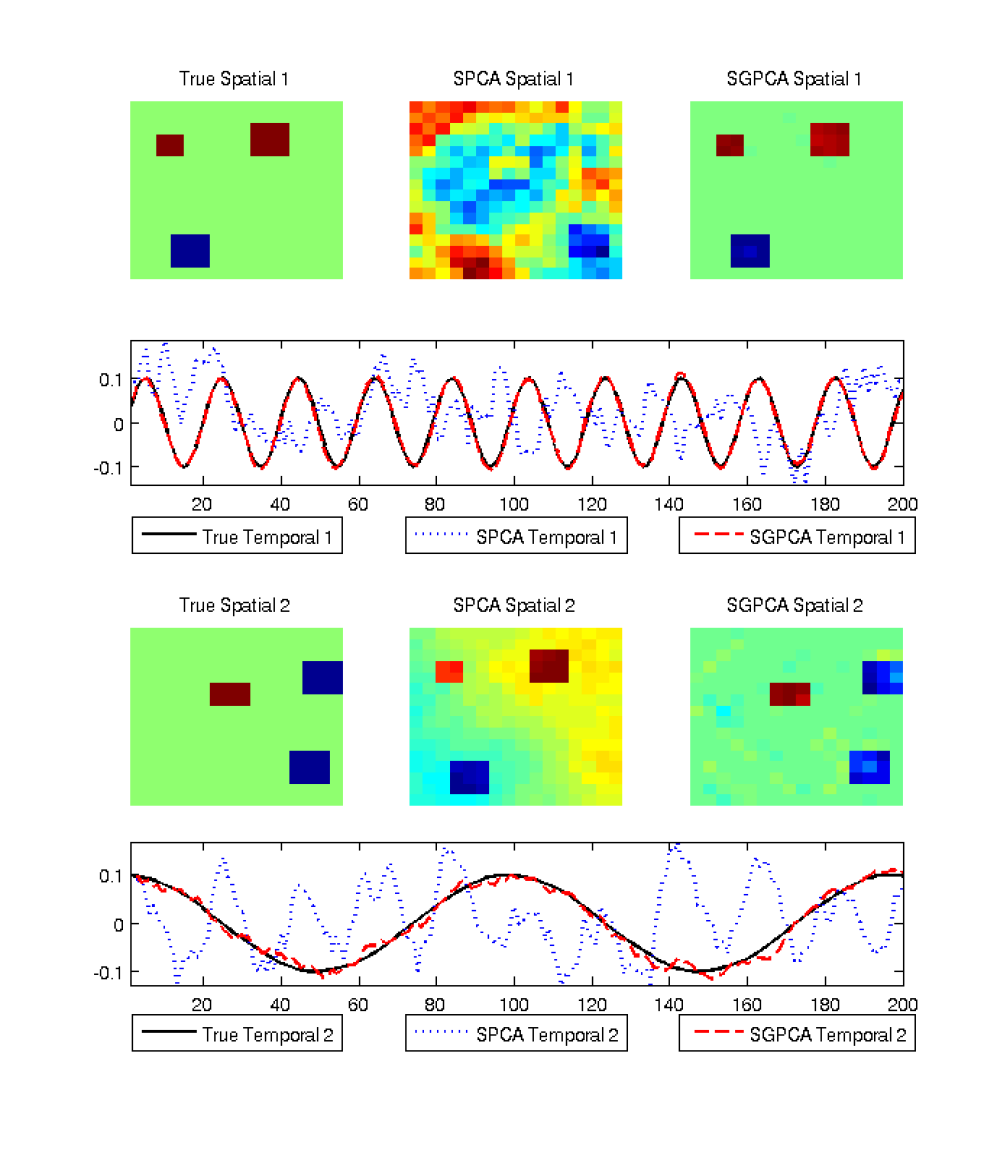
Figure 1: Example results from the spatio-temporal simulation.

Our first set of simulations is inspired by spatio-temporal neuroimaging data, and is that of the example shown in Figure  1. The two spatial signals, $\operatorname{\mathbf{U}}\in\Re^{256\times 2}$, each consist of three non-overlapping “regions of interest” on a $16\times 16$ grid. The two temporal signals, $\operatorname{\mathbf{V}}\in\Re^{200\times 2}$, are sinusoidal activation patterns with different frequencies. The signal is given by $\phi_{1}\sim N(1,\sigma^{2})$ and $\phi_{2}\sim N(0.5,\sigma^{2})$ where $\sigma$ is chosen so that the SNR = $\sigma^{2}$. The noise is simulated from an autoregressive Gaussian Markov random field. The spatial covariance, $\operatorname{\mathbf{\Sigma}}$, is that of an autoregressive process on the $16\times 16$ grid with correlation $0.9$, and the temporal covariance, $\operatorname{\mathbf{\Delta}}$, is that of an autoregressive temporal process with correlation $0.8$.

Table 1: Comparison of different quadratic operators for GPCA in the spatio-temporal simulation.

	% Var $k=1$	% Var $k=2$	MSSE $\operatorname{\mathbf{u}}_{1}$	MSSE $\operatorname{\mathbf{u}}_{2}$	MSSE $\operatorname{\mathbf{v}}_{1}$	MSSE $\operatorname{\mathbf{v}}_{2}$
$\operatorname{\mathbf{Q}}=\operatorname{\mathbf{I}}_{(m^{2})}$, $\operatorname{\mathbf{R}}=\operatorname{\mathbf{I}}_{(p)}$	57.4 (0.9)	19.1 (0.9)	0.5292 (.04)	0.6478 (.02)	0.3923 (.02)	0.4857 (.01)
$\operatorname{\mathbf{Q}}=\operatorname{\mathbf{\operatorname{\mathbf{\Sigma}}}^{-1}}$, $\operatorname{\mathbf{R}}=\operatorname{\mathbf{\Delta}^{-1}}$	75.4 (2.3)	6.6 (0.2)	0.1452 (.02)	0.3226 (.02)	0.0087 (.01)	0.0180 (.01)
$\operatorname{\mathbf{Q}}=\operatorname{\mathbf{L}}_{m,m}$, $\operatorname{\mathbf{R}}=\operatorname{\mathbf{L}}_{p}$	42.9 (2.9)	2.8 (0.1)	0.1981 (.03)	0.7972 (.02)	0.0609 (.02)	0.4334 (.02)
$\operatorname{\mathbf{Q}}=\operatorname{\mathbf{L}}_{m,m}$, $\operatorname{\mathbf{R}}=\operatorname{\mathbf{S}}_{p}$	55.8 (2.3)	14.5 (0.3)	0.1714 (.02)	0.3425 (.03)	0.0481 (.01)	0.0809 (.02)
$\operatorname{\mathbf{Q}}=\operatorname{\mathbf{S}}_{m,m}$, $\operatorname{\mathbf{R}}=\operatorname{\mathbf{L}}_{p}$	67.6 (0.7)	13.0 (0.8)	0.8320 (.02)	0.8004 (.01)	0.5414 (.01)	0.4831 (.01)
$\operatorname{\mathbf{Q}}=\operatorname{\mathbf{S}}_{m,m}$, $\operatorname{\mathbf{R}}=\operatorname{\mathbf{S}}_{p}$	60.3 (1.0)	19.3 (1.0)	0.5682 (.04)	0.6779 (.02)	0.4310 (.02)	0.5030 (.01)

The behavior demonstrated by Sparse PCA (implemented using the approach of (Shen and Huang, 2008)) and Sparse GPCA in Figure  1 where $\sigma^{2}=1$ is typical. Namely, when the signal is small and the structural noise is strong, PCA and Sparse PCA often find structural noise as the major source of variation instead of the true signal, the regions of interest and activation patterns. Even in subsequent components, PCA and Sparse PCA often find a mixture of signal and structural noise, so that the signal is never easily identified. In this example, $\operatorname{\mathbf{Q}}$ and $\operatorname{\mathbf{R}}$ are not estimated from the data and instead fixed based on the known data structure, a $16\times 16$ grid and $200$ equally spaced points respectively. In Table  1, we explore two simple possibilities for quadratic operators for this spatio-temporal data: graph Laplacians of a graph connecting nearest neighbors and a kernel smoothing matrix (using the Epanechnikov kernel) smoothing nearest neighbors. Notationally, these are denoted as $\operatorname{\mathbf{L}}_{m,m}$ for a Laplacian on a $m\times m$ mesh grid or $\operatorname{\mathbf{L}}_{p}$ for $p$ equally spaced variables; $\operatorname{\mathbf{S}}$ is denoted analogously. We present results when $\sigma^{2}=1$ in terms of variance explained and mean squared standardized error (MSSE) for 100 replicates of the simulation. Notice that the combination of a spatial Laplacian and a temporal smoother in terms of signal recovery performs nearly as well as when $\operatorname{\mathbf{Q}}$ and $\operatorname{\mathbf{R}}$ are set to the true population values and significantly better than classical PCA. Thus, quadratic operators do not necessarily need to be estimated from the data, but can instead be fixed based upon known structure. Returning to the example in Figure  1, $\operatorname{\mathbf{Q}}$ and $\operatorname{\mathbf{R}}$ are taken as a Laplacian and smoother respectively, yielding excellent recovery of the regions of interest and activation patterns.

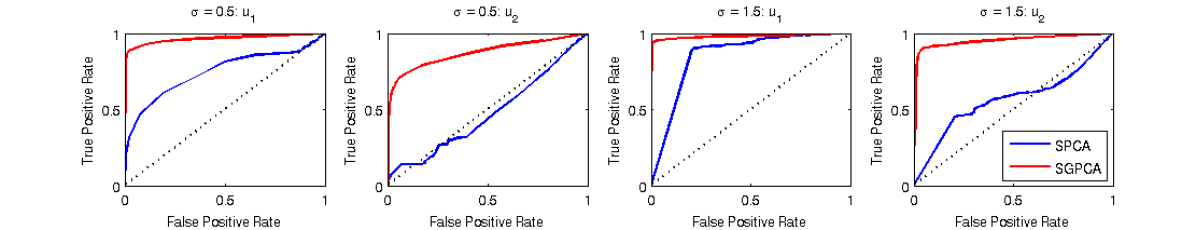
Figure 2: Average receiver-operator curves for the spatio-temporal simulation.

Next, we investigate the feature selection properties of Sparse GPCA as compared to Sparse PCA for the structured spatio-temporal simulation. Note that given the above results, $\operatorname{\mathbf{Q}}$ and $\operatorname{\mathbf{R}}$ are taken as a Laplacian and a smoothing operator for nearest neighbor graphs respectively. In Figure  2, we present mean receiver-operator curves (ROC) averaged over 100 replicates achieved by varying the regularization parameter, $\lambda$. In Table  2, we present feature selection results in terms of true and false positives when the regularization parameter $\lambda$ is fixed and estimated via the BIC method. From both of these results, we see that Sparse GPCA has major advantages over Sparse PCA. Notice also that accounting for the spatio-temporal structure through $\operatorname{\mathbf{Q}}$ and $\operatorname{\mathbf{R}}$ also yields better model selection via BIC in Table 2.

Overall, this spatio-temporal simulation has demonstrated significant advantages of GPCA and Sparse GPCA for data with low signal compared to the structural noise when the structure is fixed and known.

Table 2: Feature selection results for the spatio-temporal simulation.

		True Positive $\operatorname{\mathbf{u}}_{1}$	False Positive $\operatorname{\mathbf{u}}_{1}$	True Positive $\operatorname{\mathbf{u}}_{2}$	False Positive $\operatorname{\mathbf{u}}_{2}$
$\sigma=0.5$	Sparse PCA	0.9859 (.008)	0.9758 (.014)	0.7083 (.035)	0.7391 (.029)
	Sparse GPCA	0.9045 (.025)	0.0537 (.007)	0.7892 (.032)	0.1749 (.005)
$\sigma=1.5$	Sparse PCA	0.9927 (.004)	0.7144 (.039)	0.7592 (.034)	0.7852 (.030)
	Sparse GPCA	0.9541 (.018)	0.0292 (.005)	0.9204 (.024)	0.1572 (.004)

4.1.2 Sparse and Functional Simulations

The previous simulation example used the outer product of a sparse and smooth signal with autoregressive noise. Here, we investigate the behavior of our methods when both of the factors are either smooth or sparse and when the noise arises from differing graph structures. Specifically, we simulate noise with either a block diagonal covariance or a random graph structure in which the precision matrix arises from a graph with a random number of edges. The former has blocks of size five with off diagonal elements equal to $0.99$. The latter is generated from a graph where each vertex is connected to $n_{j}$ randomly selected vertices, where $n_{j}\overset{iid}{\sim}Poisson(3)$ for the row variables and $Poisson(1)$ for the column variables. The row and column covariances, $\operatorname{\mathbf{\Sigma}}$ and $\operatorname{\mathbf{\Delta}}$ are taken as the inverse of the nearest diagonally dominant matrix to the graph Laplacian of the row and column variables respectively. For our GMD and GPMF methods, the values of the true quadratic operators are assumed to be unknown, but the structure is known, and thus $\operatorname{\mathbf{Q}}$ and $\operatorname{\mathbf{R}}$ are taken to be the graph Laplacian. One hundred replicates of the simulations for data of dimension $100\times 100$ were performed.

Table 3: Functional Data Simulation Results.

		Squared Error	Squared Error	Squared Error
		Row Factor	Column Factor	Rank 1 Matrix
$\sigma=0.5$
	Block Diagonal Covariance
	SVD	3.670 (.121)	3.615 (.117)	67.422 (3.29)
	Two-Way Functional PCA	3.431 (.134)	3.315 (.127)	65.973 (3.41)
	GMD	1.779 (.138)	2.497 (.138)	60.687 (3.55)
	Functional GPMF	1.721 (.133)	1.721 (.144)	56.296 (2.81)
	Random Graph
	SVD	2.827 (.241)	2.729 (.234)	49.674 (1.50)
	Two-Way Functional PCA	1.968 (.258)	1.878 (.250)	49.694 (1.50)
	GMD	0.472 (.095)	1.310 (.138)	49.654 (1.51)
	Functional GPMF	0.663 (.049)	0.388 (.031)	49.666 (1.51)
$\sigma=1.0$
	Block Diagonal Covariance
	SVD	2.654 (.138)	2.532 (.143)	94.412 (6.49)
	Two-Way Functional PCA	2.426 (.142)	2.311 (.144)	92.522 (6.59)
	GMD	1.094 (.117)	1.647 (.120)	88.852 (6.73)
	Functional GPMF	1.671 (.110)	2.105 (.129)	76.864 (5.27)
	Random Graph
	SVD	2.075 (.224)	1.961 (.226)	50.392 (2.61)
	Two-Way Functional PCA	1.224 (.212)	1.187 (.206)	50.276 (2.62)
	GMD	0.338 (.075)	0.926 (.119)	50.258 (2.62)
	Functional GPMF	0.608 (.070)	0.659 (.245)	50.345 (2.60)

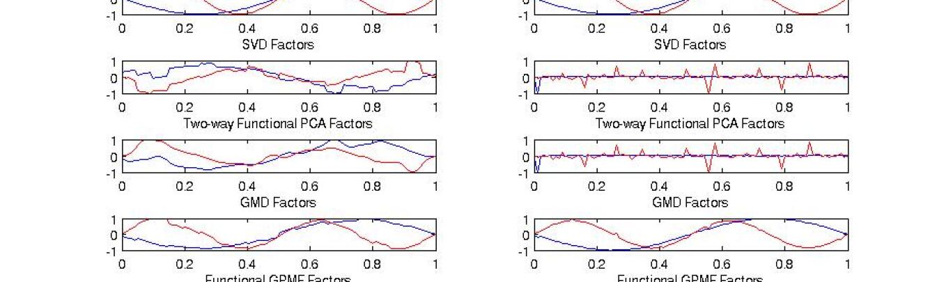
Figure 3: Example Factor Curves for Functional Data Simulation.

To test our GPMF method with the smooth $\operatorname{\mathbf{\Omega}}$-norm penalties, we simulate sinusoidal row and column factors: $\operatorname{\mathbf{u}}=sin(4\pi x)$ and $\operatorname{\mathbf{v}}=-sin(2\pi x)$ for 100 equally spaced values, $x\in[0,1]$. As the factors are fixed, the rank one signal is multiplied by $\phi\sim N(0,c^{2}\sigma^{2})$, where $c$ is chosen such that the $SNR=\sigma^{2}$. In Table 3, we compare the GMD and GPMF with smooth penalties to the SVD and the two-way functional PCA of Huang et al. (2009) in terms of squared prediction errors of the row and column factors and rank one signal. We see that both the GMD and functional GPMF outperform competing methods. Notice, however, that the functional GPMF does not always perform as well as the un-penalized GMD. In many cases, as the quadratic operators act as smoothing matrices of the noise, the GMD yields fairly smooth estimates of the factors, Figure  3.

Table 4: Sparse Factors Simulation Results.

	% True Positives	% False Positives	% True Positives	% False Positives
	Row Factor	Row Factor	Column Factor	Column Factor
Block Diagonal
Covariance
$\sigma=0.5$
Sparse PMD	76.24 (1.86)	46.20 (3.16)	79.68 (1.55)	53.23 (3.16)
Sparse GPMF	79.72 (2.45)	1.16 (0.15)	82.60 (2.57)	1.16 (0.17)
$\sigma=1.0$
Sparse PMD	87.80 (1.26)	32.80 (3.34)	88.56 (1.05)	40.93 (3.29)
Sparse GPMF	87.12 (2.19)	1.25 (0.17)	87.24 (2.21)	1.48 (0.18)
Random Graph
$\sigma=0.5$
Sparse PMD	83.56 (1.86)	39.01 (3.16)	79.44 (1.55)	33.67 (3.16)
Sparse GPMF	87.36 (2.45)	28.29 (0.15)	81.16 (2.53)	24.73 (0.17)
$\sigma=1.0$
Sparse PMD	88.04 (1.26)	46.12 (3.34)	85.36 (1.05)	48.63 (3.29)
Sparse GPMF	92.48 (2.19)	44.28 (0.17)	87.80 (2.21)	41.20 (0.18)

Finally, we test our sparse GPMF method against other sparse penalized matrix decompositions (Witten et al., 2009; Lee et al., 2010), in Table 4. In both the row and column factors, one fourth of the elements are non-zero and simulated according to $N(0,\sigma^{2})$. Here the scaling factor $\phi$ is chosen so that the $SNR=\sigma^{2}$. We compare the methods in terms of the average percent true and false positives for the row and column factors. The results indicate that our methods perform well, especially when the noise has a block diagonal covariance structure.

The three simulations indicate that our GPCA and sparse and functional GPCA methods perform well when there are two-way dependencies of the data with known structure. For the tasks of identifying regions of interest, functional patterns, and feature selection with transposable data, our methods show a substantial improvement over existing technologies.

4.2 Functional MRI Example

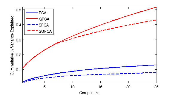
Figure 4: Cumulative proportion of variance explained by the first 25 PCs on the starplus fMRI data. Generalized PCA (GPCA) and Sparse GPCA (SGPCA) yield a significantly larger reduction in dimension that PCA and Sparse PCA (SPCA).

We demonstrate the effectiveness of our GPCA and Sparse GPCA methods on a functional MRI example. As discussed in the motivation for our methods, functional MRI data is a classic example of two-way structured data in which the nature of the noise with respect to this structure is relatively well understood. Noise in the spatial domain is related to the distance between voxels while noise in the temporal domain is often assumed to follow a autoregressive process or another classical time series process (Lindquist, 2008). Thus, when fitting our methods to this data, we consider fixed quadratic operators related to these structures and select the pair of quadratic operators yielding the largest proportion of variance explained by the first GPC. Specifically, we consider $\operatorname{\mathbf{Q}}$ in the spatial domain to be a graph Laplacian of a nearest neighbor graph connecting the voxels or a positive power of this Laplacian. In the temporal domain, we consider $\operatorname{\mathbf{R}}$ as a graph Laplacian or a positive power of a Laplacian of a chain graph or a one-dimensional smoothing matrix with a window size of five or ten. In this manner, $\operatorname{\mathbf{Q}}$ and $\operatorname{\mathbf{R}}$ are not estimated from the data and are fixed a priori based on the known two-way structure of fMRI data.

For our functional MRI example, we use a well-studied, publicly available fMRI data set where subjects were shown images and read audible sentences related to these images, a data set which refer to as the “StarPlus” data (Mitchell et al., 2004). We study data for one subject, subject number 04847, which consists of 4,698 voxels ($64\times 64\times 8$ images with masking) measured for 20 tasks, each lasting for 27 seconds, yielding 54 - 55 time points. The data was pre-processed by standardizing each voxel within each task segment. Rearranging the data yields a $4,698\times 1,098$ matrix to which we applied our dimension reduction techniques. For this data, $\operatorname{\mathbf{Q}}$ was selected to be an unweighted Laplacian and $\operatorname{\mathbf{R}}$ a kernel smoother with a window size of ten time points. In Figure 5, we present the first three PCs found by PCA, Sparse PCA, GPCA, and Sparse GPCA. Both the spatial PCs, illustrated by the eight axial slices, and the corresponding temporal PCs, with dotted red vertical lines denoting the onset of each new task period, are given. Spatial noise overwhelms PCA and Sparse PCA with large regions selected and with the corresponding time series appearing to be artifacts or scanner noise, unrelated to the experimental task. The time series of the first three GPCs and Sparse GPCs, however, exhibit a clear correlation with the task period and temporal structure characteristic of the BOLD signal. While the spatial PCs of GPCA are a bit noisy, incorporating sparsity with Sparse GPCA yields spatial maps consistent with the task in which the subject was viewing and identifying images then hearing a sentence related to that image. In particular, the first two SGPCs show bilateral occipital, left-lateralized inferior temporal, and inferior frontal activity characteristic of the well-known ”ventral stream” pathway recruited during object identification tasks (Pennick and Kana, 2012).

In Figure 4, we show the cumulative proportion of variance explained by the first 25 PCs for all our methods. Generalized PCA methods clearly exhibit an enormous advantage in terms of dimension reduction with the first GPC and SGPC explaining more sample variance than the first 20 classical PCs. As PCA is commonly used as an initial dimension reduction technique for other pattern recognition techniques, such as independent components analysis, applied to fMRI data (Lindquist, 2008), our Generalized PCA methods can offer a major advantage in this context. Overall, by directly accounting for the known two-way structure of fMRI data, our GPCA methods yield biologically and experimentally relevant results that explain much more variance than classical PCA methods.

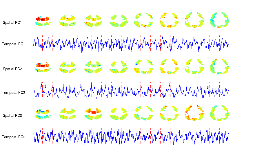
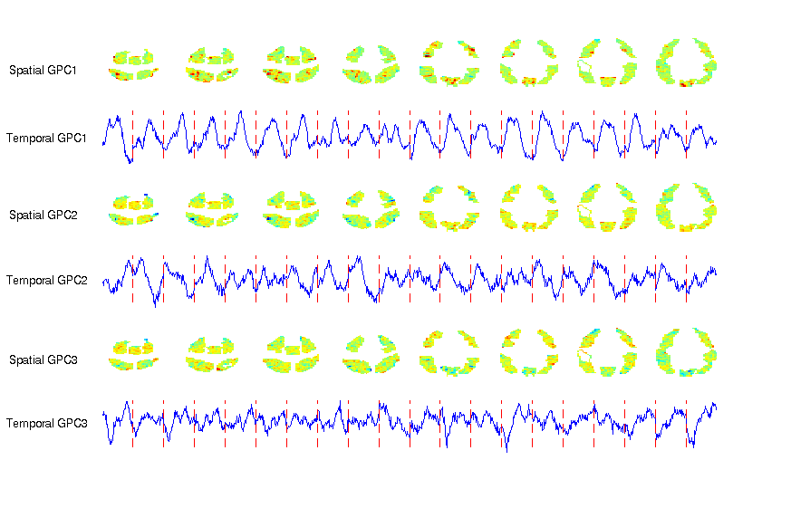
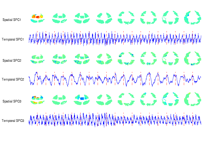
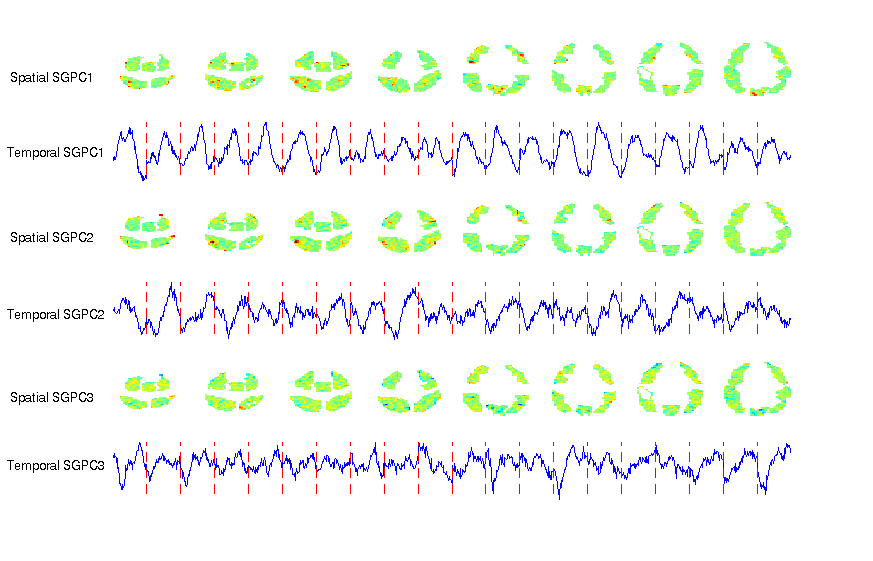
Figure 5: Eight axial slices with corresponding time series for the first three PCs of the StarPlus fMRI data for PCA (top left), Sparse PCA (bottom left), Generalized PCA (top right) and Sparse Generalized PCA (bottom right). Dotted red vertical lines in the time series denote the beginning and end of each task where an image was shown accompanied by an audible sentence that corresponded to the image. The first three spatial PCs of PCA and the first and third of Sparse PCA exhibit large patterns of spatial noise where the corresponding time series appear to be artifacts or scanner noise, unrelated to the experiment. The temporal PCs of GPCA and Sparse GPCA, on the other hand, exhibit a clear pattern with respect to the experimental task. The spatial PCs of GPCA, however are somewhat noisy, whereas when sparsity is encouraged, the spatial PCs of Sparse GPCA illustrate clear regions of activation related to the experimental task.

5 Discussion

In this paper, we have presented a general framework for incorporating structure into a matrix decomposition and a two-way penalized matrix factorization. Hence, we have provided an alternative to the SVD, PCA and regularized PCA that is appropriate for structured data. We have also developed fast computational algorithms to apply our methods to massive data such as that of functional MRIs. Along the way, we have provided results that clarify the types of penalty functions that may be employed on matrix factors that are estimated via a deflation scheme. Through simulations and a real example on fMRI data, we have shown that GPCA and regularized GPCA can be a powerful method for signal recovery and dimension reduction of high-dimensional structured data.

While we have presented a general framework permitting heteroscedastic errors in PCA and two-way regularized PCA, we currently only advocate the applied use of our methodology for structured data. Data in which measurements are taken on a grid (e.g. regularly spaced time series, spectroscopy, and image data) or on known Euclidean coordinates (e.g. environmental data, epigenetic methylation data and unequally spaced longitudinal data) have known structure which can be encoded by the quadratic operators through smoothing or graphical operators as discussed in Section 2.5. Through close connections to other non-linear unsupervised learning techniques and interpretations of GPCA as a covariance decomposition and smoothing operator, the behavior our methodology for structured data is well understood. For data that is not measured on a structured surface, however, more investigations need to be done to determine the applicability of our methods. In particular, while it may be tempting to estimate both the quadratic operators, via Allen and Tibshirani (2010) for example, and the GPCA factors, this is not an approach we advocate as separation of the noise and signal covariance structure may be confounded.

For specific applications to structured data, however, there is much future work to be done to determine how to best employ our methodology. The utility of GPCA would be greatly enhanced by data-driven methods to learn or estimate the optimal quadratic operators from certain classes of structured matrices or an inferential approach to determining the best pair of quadratic operators from a fixed set of options. With structured data in particular, methods to achieve these are not straightforward as the amount of variance explained or the matrix reconstruction error is not always a good measure of how well the structural noise is separated from the actual signal of interest (as seen in the spatio-temporal simulation, Section 4.1). Additionally as the definition of the “signal” varies from one application to another, these issues should be studied carefully for specific applications. An area of future research would then be to develop the theoretical properties of GPCA in terms of consistency or information-theoretic bounds based on classes of signal and structured noise. While these investigations are beyond the scope of this initial paper, the authors plan on exploring these issues as well as applications to specific data sets in future work.

There are many other statistical directions for future research related to our work. As many other classical multivariate analysis methods are closely related to PCA, our framework for incorporating structure and two-way regularization could be employed in methods such as canonical correlations analysis, discriminant analysis, multi-dimensional scaling, latent variable models, and clustering. Also several other statistical and machine learning techniques are based on Frobenius norms which may be altered for structured data along the lines of our approach. Additionally, there are many areas of research related to two-way regularized PCA models. Theorem 2 elucidates the classes of penalties that can be employed on PCA factors estimated via deflation that ensure algorithmic convergence. This convergence, however, is only to a local optimum. Methods are then needed to find good initializations, to estimate optimal penalty parameters, to find the relevant range of penalty parameters comprising a full solution path, and to ensure convergence to a good solution. Furthermore, asymptotic consistency of several approaches to Sparse PCA has been established (Johnstone and Lu, 2004; Amini and Wainwright, 2009; Ma, 2010), but more work needs to be done to establish consistency of two-way Sparse PCA.

Finally, our methodology work has broad implications in a wide array of applied disciplines. Massive image data is common in areas of neuroimaging, microscopy, hyperspectral imaging, remote sensing, and radiology. Other examples of high-dimensional structured data can be found in environmental and climate studies, times series and finance, engineering sensor and network data, and astronomy. Our GPCA and regularized GPCA methods can be used with these structured data sets for improved dimension reduction, signal recovery, feature selection, data visualization and exploratory data analysis.

In conclusion, we have presented a general mathematical framework for PCA and regularized PCA for massive structured data. Our methods have broad statistical and applied implications that will lead to many future areas of research.

6 Acknowledgments

The authors would like to thank Susan Holmes for bringing relevant references to our attention and Marina Vannucci for the helpful advice in the preparation of this manuscript. Additionally, we are grateful to the anonymous referees and associate editor for helpful comments and suggestions on this work. J. Taylor was partially supported by NSF DMS-0906801, and L. Grosenick was supported by NSF IGERT Award #0801700.

Appendix A Proofs

Proof 1 (Proof of Theorem  1)

We show that the GMD problem, (2.1), at $\operatorname{\mathbf{U}}^{*},\operatorname{\mathbf{D}}^{*},\operatorname{\mathbf{V}}^{*}$ is equivalent to the SVD problem, (2.1), for $\tilde{\operatorname{\mathbf{X}}}$ at $\tilde{\operatorname{\mathbf{U}}},\tilde{\operatorname{\mathbf{D}}},\tilde{\operatorname{\mathbf{V}}}$. Thus, if $\tilde{\operatorname{\mathbf{U}}},\tilde{\operatorname{\mathbf{D}}},\tilde{\operatorname{\mathbf{V}}}$ minimizes the SVD problem, (2.1), then $\operatorname{\mathbf{U}}^{*},\operatorname{\mathbf{D}}^{*},\operatorname{\mathbf{V}}^{*}$ minimizes the GMD problem, (2.1). We begin with the objectives:

$$||\operatorname{\mathbf{X}}-\operatorname{\mathbf{U}}^{*}\operatorname{\mathbf{D}}^{*}(\operatorname{\mathbf{V}}^{*})^{T}||_{\operatorname{\mathbf{Q}},\operatorname{\mathbf{R}}}^{2}=\mathrm{tr}\left(\operatorname{\mathbf{Q}}\operatorname{\mathbf{X}}\operatorname{\mathbf{R}}\operatorname{\mathbf{X}}^{T}\right)-2\mathrm{tr}\left(\operatorname{\mathbf{Q}}\operatorname{\mathbf{U}}^{*}\operatorname{\mathbf{D}}^{*}(\operatorname{\mathbf{V}}^{*})^{T}\operatorname{\mathbf{R}}\operatorname{\mathbf{X}}^{T}\right)$$

$$\qquad\qquad+\mathrm{tr}\left(\operatorname{\mathbf{Q}}\operatorname{\mathbf{U}}^{*}\operatorname{\mathbf{D}}^{*}(\operatorname{\mathbf{V}}^{*})^{T}\operatorname{\mathbf{R}}\operatorname{\mathbf{V}}^{*}(\operatorname{\mathbf{D}}^{*})^{T}(\operatorname{\mathbf{U}}^{*})^{T}\right)$$

$$\qquad=\mathrm{tr}\left(\tilde{\operatorname{\mathbf{Q}}}\tilde{\operatorname{\mathbf{Q}}}^{T}\operatorname{\mathbf{X}}\tilde{\operatorname{\mathbf{R}}}\tilde{\operatorname{\mathbf{R}}}^{T}\operatorname{\mathbf{X}}^{T}\right)-2\mathrm{tr}\left(\tilde{\operatorname{\mathbf{Q}}}\tilde{\operatorname{\mathbf{Q}}}^{T}\tilde{\operatorname{\mathbf{Q}}}^{-1}\tilde{\operatorname{\mathbf{U}}}\tilde{\operatorname{\mathbf{D}}}\tilde{\operatorname{\mathbf{V}}}^{T}(\tilde{\operatorname{\mathbf{R}}}^{-1})^{T}\tilde{\operatorname{\mathbf{R}}}\tilde{\operatorname{\mathbf{R}}}^{T}\operatorname{\mathbf{X}}^{T}\tilde{\operatorname{\mathbf{Q}}}\right)$$

$$\qquad\qquad+\mathrm{tr}\left(\tilde{\operatorname{\mathbf{Q}}}\tilde{\operatorname{\mathbf{Q}}}^{T}\tilde{\operatorname{\mathbf{Q}}}^{-1}\tilde{\operatorname{\mathbf{U}}}\tilde{\operatorname{\mathbf{D}}}\tilde{\operatorname{\mathbf{V}}}^{T}(\tilde{\operatorname{\mathbf{R}}}^{-1})^{T}\tilde{\operatorname{\mathbf{R}}}\tilde{\operatorname{\mathbf{R}}}^{T}\tilde{\operatorname{\mathbf{R}}}^{-1}\tilde{\operatorname{\mathbf{V}}}\tilde{\operatorname{\mathbf{D}}}^{T}\tilde{\operatorname{\mathbf{U}}}^{T}\tilde{\operatorname{\mathbf{Q}}}^{-1}\right)$$

$$\qquad=\mathrm{tr}\left(\tilde{\operatorname{\mathbf{X}}}\tilde{\operatorname{\mathbf{X}}}^{T}\right)-2\mathrm{tr}\left(\tilde{\operatorname{\mathbf{U}}}\tilde{\operatorname{\mathbf{D}}}\tilde{\operatorname{\mathbf{V}}}^{T}\tilde{\operatorname{\mathbf{X}}}^{T}\right)+\mathrm{tr}\left(\tilde{\operatorname{\mathbf{U}}}\tilde{\operatorname{\mathbf{D}}}\tilde{\operatorname{\mathbf{V}}}^{T}\tilde{\operatorname{\mathbf{V}}}\tilde{\operatorname{\mathbf{D}}}^{T}\tilde{\operatorname{\mathbf{U}}}^{T}\right)=||\tilde{\operatorname{\mathbf{X}}}-\tilde{\operatorname{\mathbf{U}}}\tilde{\operatorname{\mathbf{D}}}\tilde{\operatorname{\mathbf{V}}}^{T}||_{F}^{2}.$$

One can easily verify that the constraint regions are equivalent: $(\operatorname{\mathbf{U}}^{*})^{T}\operatorname{\mathbf{Q}}\operatorname{\mathbf{U}}^{*}=\tilde{\operatorname{\mathbf{U}}}^{T}\tilde{\operatorname{\mathbf{Q}}}^{-1}\operatorname{\mathbf{Q}}(\tilde{\operatorname{\mathbf{Q}}}^{-1})^{T}\tilde{\operatorname{\mathbf{U}}}=\tilde{\operatorname{\mathbf{U}}}^{T}\tilde{\operatorname{\mathbf{U}}}$ and similarly for $\operatorname{\mathbf{V}}$ and $\operatorname{\mathbf{R}}$. This completes the proof.

Proof 2 (Proof of Corollaries to Theorem  1)

These results follow from the properties of the SVD (Eckart and Young, 1936; Horn and Johnson, 1985; Golub and Van Loan, 1996) and the relationship between the GMD and SVD given in Theorem  1. For Corollary  2, we use the fact that $\mathrm{rank}(\operatorname{\mathbf{A}}\operatorname{\mathbf{B}})\leq\mathrm{min}\{\mathrm{rank}(\operatorname{\mathbf{A}}),\mathrm{rank}(\operatorname{\mathbf{B}})\}$ for any two matrices $\operatorname{\mathbf{A}}$ and $\operatorname{\mathbf{B}}$; equality holds if $range(\operatorname{\mathbf{A}})\cap null(\operatorname{\mathbf{B}})=\emptyset$. Then, $\mathrm{rank}(\tilde{\operatorname{\mathbf{X}}})=k=\mathrm{min}\{\mathrm{rank}(\operatorname{\mathbf{X}}),\mathrm{rank}(\operatorname{\mathbf{Q}}),\mathrm{rank}(\operatorname{\mathbf{R}})\}$.

Proof 3 (Proof of Proposition  1)

We show that the updates of $\operatorname{\mathbf{u}}$ and $\operatorname{\mathbf{v}}$ in the GMD Algorithm are equivalent to the updates in the power method for computing the SVD of $\tilde{\operatorname{\mathbf{X}}}$. Writing the update for $\operatorname{\mathbf{u}}_{k}$ in terms of$\tilde{\operatorname{\mathbf{X}}}$, $\tilde{\operatorname{\mathbf{u}}}$, and $\tilde{\operatorname{\mathbf{v}}}$ (suppressing the index $k$), we have:

$$(\tilde{\operatorname{\mathbf{Q}}}^{-1})^{T}\tilde{\operatorname{\mathbf{u}}} =\frac{((\tilde{\operatorname{\mathbf{Q}}}^{-1})^{T}\tilde{\operatorname{\mathbf{X}}}\tilde{\operatorname{\mathbf{R}}}^{-1})\operatorname{\mathbf{R}}(\tilde{\operatorname{\mathbf{R}}}^{-1})^{T}\tilde{\operatorname{\mathbf{v}}}}{||((\tilde{\operatorname{\mathbf{Q}}}^{-1})^{T}\tilde{\operatorname{\mathbf{X}}}\tilde{\operatorname{\mathbf{R}}}^{-1})\operatorname{\mathbf{R}}(\tilde{\operatorname{\mathbf{R}}}^{-1})^{T}\tilde{\operatorname{\mathbf{v}}}||_{\operatorname{\mathbf{Q}}}},\Rightarrow\tilde{\operatorname{\mathbf{u}}} =\frac{\tilde{\operatorname{\mathbf{X}}}\tilde{\operatorname{\mathbf{v}}}}{\sqrt{\tilde{\operatorname{\mathbf{v}}}^{T}\tilde{\operatorname{\mathbf{X}}}^{T}\tilde{\operatorname{\mathbf{Q}}}^{-1}\operatorname{\mathbf{Q}}(\tilde{\operatorname{\mathbf{Q}}}^{-1})^{T}\tilde{\operatorname{\mathbf{X}}}\tilde{\operatorname{\mathbf{v}}}}}=\frac{\tilde{\operatorname{\mathbf{X}}}\tilde{\operatorname{\mathbf{v}}}}{||\tilde{\operatorname{\mathbf{X}}}\tilde{\operatorname{\mathbf{v}}}||_{2}}.$$

Notice that this last form in $\tilde{\operatorname{\mathbf{u}}}$ is that of the power method for computing the SVD of $\tilde{\operatorname{\mathbf{X}}}$ (Golub and Van Loan, 1996). A similar calculation for $\operatorname{\mathbf{v}}$ yields an analogous form. Therefore, the GMD Algorithm is equivalent to the algorithm which converges to the SVD of $\tilde{\operatorname{\mathbf{X}}}$.

Proof 4 (Proof of Proposition  2)

We show that the objective and constraints in (3) at the GMD solution are the same as that of the rank $k$ PCA problem for $\tilde{\operatorname{\mathbf{X}}}$. (For simplicity of notation, we suppress the index $k$ in the calculation.)

$$\operatorname{\mathbf{v}}^{T}\operatorname{\mathbf{R}}\operatorname{\mathbf{X}}^{T}\operatorname{\mathbf{Q}}\operatorname{\mathbf{X}}\operatorname{\mathbf{R}}\operatorname{\mathbf{v}} =\tilde{\operatorname{\mathbf{v}}}^{T}(\tilde{\operatorname{\mathbf{R}}}^{-1})^{T}\operatorname{\mathbf{R}}\tilde{\operatorname{\mathbf{R}}}^{-1}\tilde{\operatorname{\mathbf{X}}}(\tilde{\operatorname{\mathbf{Q}}}^{-1})^{T}\operatorname{\mathbf{Q}}\tilde{\operatorname{\mathbf{Q}}}^{-1}\tilde{\operatorname{\mathbf{X}}}(\tilde{\operatorname{\mathbf{R}}}^{-1})^{T}\operatorname{\mathbf{R}}\tilde{\operatorname{\mathbf{R}}}^{-1}\tilde{\operatorname{\mathbf{v}}}=\tilde{\operatorname{\mathbf{v}}}^{T}\tilde{\operatorname{\mathbf{X}}}^{T}\tilde{\operatorname{\mathbf{X}}}\tilde{\operatorname{\mathbf{v}}}$$

$$\operatorname{\mathbf{v}}^{T}\operatorname{\mathbf{R}}\operatorname{\mathbf{v}} =\tilde{\operatorname{\mathbf{v}}}^{T}(\tilde{\operatorname{\mathbf{R}}}^{-1})^{T}\operatorname{\mathbf{R}}\tilde{\operatorname{\mathbf{R}}}^{-1}\tilde{\operatorname{\mathbf{v}}}=\tilde{\operatorname{\mathbf{v}}}^{T}\tilde{\operatorname{\mathbf{v}}}.$$

Then, the left singular vector, $\tilde{\operatorname{\mathbf{v}}}$, that maximizes the PCA problem, is the same as the left GMD factor that maximizes (3).

Proof 5 (Proof of Corollary  5)

This result follows from the relationship of the GMD and GPCA to the SVD and PCA. Recall that for PCA, the amount of variance explained by the $k^{th}$ PC is given by $d_{k}^{2}/||\operatorname{\mathbf{X}}||_{F}^{2}$ where $d_{k}$ is the $k^{th}$ singular value of $\operatorname{\mathbf{X}}$. Then, notice that the stated result is equivalent to the proportion of variance explained by the $k^{th}$ singular vector of $\tilde{\operatorname{\mathbf{X}}}$: $\tilde{d}_{k}^{2}/\mathrm{tr}(\tilde{\operatorname{\mathbf{X}}}\tilde{\operatorname{\mathbf{X}}}^{T})=d_{k}^{2}/\mathrm{tr}(\operatorname{\mathbf{Q}}\operatorname{\mathbf{X}}\operatorname{\mathbf{R}}\operatorname{\mathbf{X}}^{T})$.

Proof 6 (Proof of Theorem  2)

We will show that the result holds for $\operatorname{\mathbf{v}}$, and the argument for $\operatorname{\mathbf{u}}$ is analogous. Consider optimization of (4) with respect to $\operatorname{\mathbf{v}}$ with $\operatorname{\mathbf{u}}$ fixed at $\operatorname{\mathbf{u}}^{\prime}$. The problem is concave in $\operatorname{\mathbf{v}}$ and there exists a strictly feasible point, hence Slater’s condition holds and the KKT conditions are necessary and sufficient for optimality. Letting $\operatorname{\mathbf{y}}=\operatorname{\mathbf{X}}^{T}\operatorname{\mathbf{Q}}\operatorname{\mathbf{u}}$, these are given by: $\operatorname{\mathbf{R}}\operatorname{\mathbf{y}}-\operatorname*{\lambda_{\mathbf{v}}}\nabla P_{1}(\operatorname{\mathbf{v}}^{*})-2\gamma^{*}\operatorname{\mathbf{R}}\operatorname{\mathbf{v}}^{*}=0$ and $\gamma^{*}((\operatorname{\mathbf{v}}^{*})^{T}\operatorname{\mathbf{R}}\operatorname{\mathbf{v}}^{*}-1)=0$. Here, $\nabla P_{1}(\operatorname{\mathbf{v}}^{*})$ is a subgradient of $P_{1}()$ with respect to $\operatorname{\mathbf{v}}^{*}$. Now, consider the following solution to the penalized regression problem: $\hat{\operatorname{\mathbf{v}}}=\operatorname*{\mathrm{argmin}}_{\operatorname{\mathbf{v}}}\{\frac{1}{2}||\operatorname{\mathbf{y}}-\operatorname{\mathbf{v}}||_{\operatorname{\mathbf{R}}}^{2}+\operatorname*{\lambda_{\mathbf{v}}}P_{1}(\operatorname{\mathbf{v}})\}$. This solution must satisfy the subgradient conditions. Hence, $\forall\ c>0$, we have:

$$0=\operatorname{\mathbf{R}}\operatorname{\mathbf{y}}-\operatorname*{\lambda_{\mathbf{v}}}\nabla P_{1}(\hat{\operatorname{\mathbf{v}}})-\operatorname{\mathbf{R}}\hat{\operatorname{\mathbf{v}}}=\operatorname{\mathbf{R}}\operatorname{\mathbf{y}}-\operatorname*{\lambda_{\mathbf{v}}}\nabla P_{1}(\hat{\operatorname{\mathbf{v}}})-\operatorname{\mathbf{R}}(c\hat{\operatorname{\mathbf{v}}})\frac{1}{c}=\operatorname{\mathbf{R}}\operatorname{\mathbf{y}}-\operatorname*{\lambda_{\mathbf{v}}}\nabla P_{1}(\tilde{\operatorname{\mathbf{v}}})-\operatorname{\mathbf{R}}\tilde{\operatorname{\mathbf{v}}}\frac{1}{c},$$

where $\tilde{\operatorname{\mathbf{v}}}=c\hat{\operatorname{\mathbf{v}}}$. The last step follows because since $P_{1}()$ is convex and homogeneous of order one, $\nabla P_{1}(x)=\nabla P_{1}(cx)\ \ \forall\ c>0$.

Let us take $c=1/||\hat{\operatorname{\mathbf{v}}}||_{\operatorname{\mathbf{R}}}$; we see that this satisfies $c>0$. Then, letting $\gamma^{*}=\frac{1}{2c}=||\hat{\operatorname{\mathbf{v}}}||_{\operatorname{\mathbf{R}}}/2$, we see that the subgradient condition of (4) is equivalent to that of the penalized regression problem. Putting these together, we see that the pair $(\operatorname{\mathbf{v}}^{*}=\hat{\operatorname{\mathbf{v}}}/||\hat{\operatorname{\mathbf{v}}}||_{\operatorname{\mathbf{R}}},\gamma^{*}=||\hat{\operatorname{\mathbf{v}}}||_{\operatorname{\mathbf{R}}}/2)$ satisfies the KKT conditions and is hence the optimal solution. Notice that $\gamma^{*}=0$ only if $||\hat{\operatorname{\mathbf{v}}}||_{\operatorname{\mathbf{R}}}=0$. From our discussion of the quadratic norm, recall that this can only occur if $\hat{\operatorname{\mathbf{v}}}\in null(\operatorname{\mathbf{R}})$ or $\hat{\operatorname{\mathbf{v}}}=0$. Since we exclude the former by assumption, this implies that if $\hat{\operatorname{\mathbf{v}}}=0$, then $\gamma^{*}=0$ and the inequality constraint in (4) is not tight. In this case, it is easy to verify that the pair $(\operatorname{\mathbf{v}}^{*}=0,\gamma^{*}=0)$ satisfy the KKT conditions. Thus, we have proven the desired result.

Proof 7 (Proof of Claim  1)

Examining the subgradient condition, we have that $\hat{\operatorname{\mathbf{v}}}=\operatorname{\mathbf{y}}-\lambda\operatorname{\mathbf{R}}^{-1}\mathbf{1}_{(p)}\nabla P(\hat{\operatorname{\mathbf{v}}})$. This can be written as such because the subgradient equation is separable in the elements of $\hat{\operatorname{\mathbf{v}}}$ when $\operatorname{\mathbf{R}}$ is diagonal. Then, it follows that soft thresholding the elements of $\operatorname{\mathbf{y}}$ with the penalty vector $\lambda\operatorname{\mathbf{R}}^{-1}\mathbf{1}_{(p)}$ solves the subgradient equation.

Proof 8 (Proof of Claim  2)

We can write the problem, $\frac{1}{2}||\operatorname{\mathbf{y}}-\operatorname{\mathbf{v}}||_{\operatorname{\mathbf{R}}}^{2}+\operatorname*{\lambda_{\mathbf{v}}}||\operatorname{\mathbf{v}}||_{1}$, as a lasso regression problem in terms of $\tilde{\operatorname{\mathbf{R}}}$, $\frac{1}{2}||\tilde{\operatorname{\mathbf{R}}}^{T}\operatorname{\mathbf{y}}-\tilde{\operatorname{\mathbf{R}}}^{T}\operatorname{\mathbf{v}}||_{2}^{2}+\operatorname*{\lambda_{\mathbf{v}}}||\operatorname{\mathbf{v}}||_{1}$. Friedman et al. (2007) established that the lasso regression problem can be solved by iterative coordinate-descent. Then, optimizing with respect to each coordinate, $\operatorname{\mathbf{v}}_{j}$: $\hat{\operatorname{\mathbf{v}}}_{j}=\frac{1}{\tilde{\operatorname{\mathbf{R}}}_{rj}^{T}\tilde{\operatorname{\mathbf{R}}}_{rj}}S\left(\tilde{\operatorname{\mathbf{R}}}_{rj}^{T}\tilde{\operatorname{\mathbf{R}}}\operatorname{\mathbf{y}}-\tilde{\operatorname{\mathbf{R}}}_{rj}^{T}\tilde{\operatorname{\mathbf{R}}}_{r,\neq j}\hat{\operatorname{\mathbf{v}}}_{\neq j},\lambda\right)$. Now, several of these quantities can be written in terms of $\operatorname{\mathbf{R}}$ so that $\tilde{\operatorname{\mathbf{R}}}$ does not need to be computed and stored: $\tilde{\operatorname{\mathbf{R}}}_{rj}^{T}\tilde{\operatorname{\mathbf{R}}}_{rj}=\operatorname{\mathbf{R}}_{jj}$, $\tilde{\operatorname{\mathbf{R}}}_{rj}^{T}\tilde{\operatorname{\mathbf{R}}}=\operatorname{\mathbf{R}}_{rj}$, and $\tilde{\operatorname{\mathbf{R}}}_{rj}^{T}\tilde{\operatorname{\mathbf{R}}}_{r,\neq j}=\operatorname{\mathbf{R}}_{j,\neq j}$. Putting these together, we have the desired result.

Proof 9 (Proof of Proposition  3)

We will show that Algorithm  2 uses a generalized gradient descent method converging to the minimum of the $\operatorname{\mathbf{\Omega}}$-norm generalized regression problem. First, since $\operatorname{\mathbf{B}}$ is full rank, there is a one to one mapping between $\operatorname{\mathbf{v}}$ and $\operatorname{\mathbf{w}}$. Thus, any $(\operatorname{\mathbf{w}}^{*},\eta^{*})$ minimizing $f(\operatorname{\mathbf{w}},\eta)=\frac{1}{2}||\operatorname{\mathbf{y}}-\operatorname{\mathbf{\Omega}}^{-1/2}\operatorname{\mathbf{w}}-\mathbf{N}\eta||_{\operatorname{\mathbf{R}}}^{2}+\operatorname*{\lambda_{\mathbf{v}}}||\operatorname{\mathbf{w}}||_{2}$ yields $\operatorname{\mathbf{v}}^{*}=\operatorname{\mathbf{B}}\begin{pmatrix}\operatorname{\mathbf{w}}^{*}\\ \eta^{*}\end{pmatrix}$ which minimizes the $\operatorname{\mathbf{\Omega}}$-norm generalized regression problem.

Now, let us call the first and second terms in $f(\operatorname{\mathbf{w}},\eta)$, $g(\operatorname{\mathbf{w}},\eta)$ and $h(\operatorname{\mathbf{w}},\eta)$ respectively. Then, $h(\operatorname{\mathbf{w}},\eta)$ and $g(\operatorname{\mathbf{w}},\eta)$ are obviously convex and $g(\operatorname{\mathbf{w}},\eta)$ is Lipschitz with a Lipschitz constant upper bounded by $\|\operatorname{\mathbf{B}}^{T}\operatorname{\mathbf{R}}\operatorname{\mathbf{B}}\|_{op}$. To see this, note that $\nabla g(\operatorname{\mathbf{w}},\eta)=-\operatorname{\mathbf{B}}^{T}\operatorname{\mathbf{R}}\left(\operatorname{\mathbf{y}}-\operatorname{\mathbf{B}}\begin{pmatrix}\operatorname{\mathbf{w}}\\ \eta\end{pmatrix}\right)$ is linear in $(\operatorname{\mathbf{w}},\eta)$. Therefore, we can take the operator norm of the linear part as a Lipschitz constant. We also note that $f(\operatorname{\mathbf{w}}\eta)$ is separable in $\operatorname{\mathbf{w}}$ and $\eta$ and hence block-wise coordinate descent can be employed.

Putting all of these together, the generalized gradient update for $\operatorname{\mathbf{w}}$ and the update for $\eta$ that converge to the minimum of the $\operatorname{\mathbf{\Omega}}$-norm penalized regression problem is given by the following updates (Vandenberghe, 2009; Beck and Teboulle, 2009):

$$\operatorname{\mathbf{w}}^{(t+1)}=\operatorname*{\mathrm{argmin}}_{\operatorname{\mathbf{w}}}\left\{\frac{L}{2}\left\|\operatorname{\mathbf{w}}-\left(\operatorname{\mathbf{w}}^{(t)}+\frac{1}{L}\operatorname{\mathbf{B}}^{T}\operatorname{\mathbf{R}}\left(\operatorname{\mathbf{y}}-\operatorname{\mathbf{\Omega}}^{-1/2}\operatorname{\mathbf{w}}^{(t)}-\mathbf{N}\eta^{(t)}\right)\right)\right\|_{2}^{2}+\operatorname*{\lambda_{\mathbf{v}}}||\operatorname{\mathbf{w}}||_{2}\right\}$$

$$\eta^{(t+1)}=\operatorname*{\mathrm{argmin}}_{\eta}f(\operatorname{\mathbf{w}}^{(t+1)},\eta).$$

Notice that the first minimization problem is of the form of the group lasso regression problem with an identity predictor matrix. The solution to this is problem given in Yuan and Lin (2006) and is the update in Step (b) of Algorithm 2. The second minimization problem is a simple linear regression and is the update in Step (c). This completes the proof.

Proof 10 (Proof of Proposition  4)

This result follows from an argument in Shen and Huang (2008). Namely, since our regularized GPCA formulation does not impose orthogonality of subsequent factors in the $\operatorname{\mathbf{Q}},\operatorname{\mathbf{R}}$-norm, the effect of the first $k$ factors must be projected out of the data to compute the cumulative proportion of variance explained. Shen and Huang (2008) showed that for Sparse PCA with a penalty on $\operatorname{\mathbf{v}}$, the total variance explained is given by $\mathrm{tr}(\operatorname{\mathbf{X}}_{k}\operatorname{\mathbf{X}}_{k}^{T})$ where $\operatorname{\mathbf{X}}_{k}=\operatorname{\mathbf{X}}\operatorname{\mathbf{P}}_{k}^{(\operatorname{\mathbf{V}})}=\operatorname{\mathbf{X}}\operatorname{\mathbf{V}}_{k}(\operatorname{\mathbf{V}}_{k}^{T}\operatorname{\mathbf{V}}_{k})^{-1}\operatorname{\mathbf{V}}_{k}^{T}$ with $\operatorname{\mathbf{V}}_{k}=[\operatorname{\mathbf{v}}_{1}\ \ldots\ \operatorname{\mathbf{v}}_{k}]$. When penalties are incorporated on both factors, one must define $\operatorname{\mathbf{X}}_{k}=\operatorname{\mathbf{P}}_{k}^{(\operatorname{\mathbf{U}})}\operatorname{\mathbf{X}}\operatorname{\mathbf{P}}_{k}^{(\operatorname{\mathbf{V}})}$. We show that the total proportion of variance explained (the numerator of our stated result) is equivalent to $\mathrm{tr}(\tilde{\operatorname{\mathbf{X}}}_{k}\tilde{\operatorname{\mathbf{X}}}_{k})$, where $\tilde{\operatorname{\mathbf{X}}}_{k}$ is equivalent to that as defined in Theorem  1. First, notice that $\operatorname{\mathbf{P}}_{k}^{(\operatorname{\mathbf{U}})}=\tilde{\operatorname{\mathbf{Q}}}^{-1}\tilde{\operatorname{\mathbf{U}}}_{k}(\tilde{\operatorname{\mathbf{U}}}_{k}^{T}(\tilde{\operatorname{\mathbf{Q}}}^{-1})^{T}\operatorname{\mathbf{Q}}\tilde{\operatorname{\mathbf{Q}}}^{-1}\tilde{\operatorname{\mathbf{U}}}_{k})^{-1}\tilde{\operatorname{\mathbf{U}}}_{k}^{T}(\tilde{\operatorname{\mathbf{Q}}}^{-1})^{T}=\tilde{\operatorname{\mathbf{Q}}}^{-1}\operatorname{\mathbf{P}}_{k}^{(\tilde{\operatorname{\mathbf{U}}})}(\tilde{\operatorname{\mathbf{Q}}}^{-1})^{T}$ and equivalently, $\operatorname{\mathbf{P}}_{k}^{(\operatorname{\mathbf{V}})}=\tilde{\operatorname{\mathbf{R}}}^{-1}\operatorname{\mathbf{P}}_{k}^{(\tilde{\operatorname{\mathbf{V}}})}(\tilde{\operatorname{\mathbf{R}}}^{-1})^{T}$. Then, $\operatorname{\mathbf{X}}_{k}=\operatorname{\mathbf{P}}_{k}^{(\operatorname{\mathbf{U}})}\operatorname{\mathbf{Q}}\operatorname{\mathbf{X}}\operatorname{\mathbf{R}}\operatorname{\mathbf{P}}_{k}^{(\operatorname{\mathbf{V}})}=\tilde{\operatorname{\mathbf{Q}}}^{-1}\operatorname{\mathbf{P}}_{k}^{(\tilde{\operatorname{\mathbf{U}}})}\tilde{\operatorname{\mathbf{X}}}\operatorname{\mathbf{P}}_{k}^{(\tilde{\operatorname{\mathbf{V}}})}\tilde{\operatorname{\mathbf{R}}}^{-1}$, and we have that
$\mathrm{tr}(\operatorname{\mathbf{Q}}\operatorname{\mathbf{X}}_{k}\operatorname{\mathbf{R}}\operatorname{\mathbf{X}}_{k}^{T})=\tilde{\operatorname{\mathbf{Q}}}\tilde{\operatorname{\mathbf{Q}}}^{T}\tilde{\operatorname{\mathbf{Q}}}^{-1}\operatorname{\mathbf{P}}_{k}^{(\tilde{\operatorname{\mathbf{U}}})}\tilde{\operatorname{\mathbf{X}}}\operatorname{\mathbf{P}}_{k}^{(\tilde{\operatorname{\mathbf{V}}})}\tilde{\operatorname{\mathbf{R}}}^{-1}\tilde{\operatorname{\mathbf{R}}}\tilde{\operatorname{\mathbf{R}}}^{T}(\tilde{\operatorname{\mathbf{R}}}^{-1})^{T}\operatorname{\mathbf{P}}_{k}^{(\tilde{\operatorname{\mathbf{V}}})}\tilde{\operatorname{\mathbf{X}}}^{T}\operatorname{\mathbf{P}}_{k}^{(\tilde{\operatorname{\mathbf{U}}})}(\tilde{\operatorname{\mathbf{Q}}}^{-1})^{T}=\mathrm{tr}(\tilde{\operatorname{\mathbf{X}}}_{k}\tilde{\operatorname{\mathbf{X}}}_{k}^{T})$, thus giving the desired result.

Proof 11 (Proof of Claim  3)

Lee et al. (2010) show that estimating $\operatorname{\mathbf{v}}$ in the manner described in our GPMF framework is analogous to a penalized regression problem with a sample size of $np$ and $p$ variables. Using this and assuming that the noise term of the penalized regression problem is unknown, we arrive at the given form of the BIC. Notice that the sums of squares loss function is replaced by the $\operatorname{\mathbf{Q}},\operatorname{\mathbf{R}}$-norm loss function of the GMD model.

References

- Allen and Tibshirani (2010) Allen, G. I. and R. Tibshirani (2010). Transposable regularized covariance models with an application to missing data imputation. Annals of Applied Statistics 4(2), 764–790.
- Amini and Wainwright (2009) Amini, A. and M. Wainwright (2009). High-dimensional analysis of semidefinite relaxations for sparse principal components. The Annals of Statistics 37(5B), 2877–2921.
- Beck and Teboulle (2009) Beck, A. and M. Teboulle (2009). A fast iterative shrinkage-thresholding algorithm for linear inverse problems. SIAM Journal on Imaging Sciences 2(1), 183–202.
- Becker et al. (2009) Becker, S., J. Bobin, and E. J. Candès (2009, April). NESTA: a fast and accurate First-Order method for sparse recovery. Technical report, California Institute of Technology.
- Becker et al. (2010) Becker, S., E. J. Candès, and M. Grant (2010, September). Templates for convex cone problems with applications to sparse signal recovery. Technical report, Stanford University.
- Boyd and Vandenberghe (2004) Boyd, S. and L. Vandenberghe (2004). Convex Optimization. Cambridge University Press.
- Buja and Eyuboglu (1992) Buja, A. and N. Eyuboglu (1992). Remarks on parallel analysis. Multivariate behavioral research 27(4), 509–540.
- Calhoun et al. (2001) Calhoun, V., T. Adali, G. Pearlson, and J. Pekar (2001). A method for making group inferences from functional MRI data using independent component analysis. Human Brain Mapping 14(3), 140–151.
- Chen and Buja (2009) Chen, L. and A. Buja (2009). Local multidimensional scaling for nonlinear dimension reduction, graph drawing, and proximity analysis. Journal of the American Statistical Association 104(485), 209–219.
- Dray and Dufour (2007) Dray, S. and A. Dufour (2007). The ade4 package: implementing the duality diagram for ecologists. Journal of Statistical Software 22(4), 1–20.
- Eckart and Young (1936) Eckart, C. and G. Young (1936). The approximation of one matrix by another of lower rank. Psychometrika 1(3), 211–218.
- Escoufier (1977) Escoufier, Y. (1977). Operators related to a data matrix. Recent Developments in Statistics, 125–131.
- Escoufier (1987) Escoufier, Y. (1987). The duality diagramm: a means of better practical applications. Development in numerical ecology, 139–156.
- Escoufier (2006) Escoufier, Y. (2006). Operator related to a data matrix: a survey. Compstat 2006-Proceedings in Computational Statistics, 285–297.
- Fan and Li (2001a) Fan, J. and R. Li (2001a). Variable selection via nonconcave penalized likelihood and its oracle properties. Journal of the American Statistical Association 96(456), 1348–1360.
- Fan and Li (2001b) Fan, J. and R. Li (2001b). Variable selection via nonconcave penalized likelihood and its oracle properties. Journal of the American Statistical Association 96(456), 1348–1360.
- Friedman et al. (2007) Friedman, J., T. Hastie, H. Hoefling, and R. Tibshirani (2007). Pathwise coordinate optimization. Annals of Applied Statistics 1(2), 302–332.
- Friedman et al. (2010) Friedman, J., T. Hastie, and R. Tibshirani (2010). Regularization paths for generalized linear models via coordinate descent. Journal of statistical software 33(1), 1.
- Friston et al. (1999) Friston, K., J. Phillips, D. Chawla, and C. Buchel (1999). Revealing interactions among brain systems with nonlinear PCA. Human brain mapping 8(2-3), 92–97.
- Galbraith and Galbraith (1974) Galbraith, R. and J. Galbraith (1974). On the inverses of some patterned matrices arising in the theory of stationary time series. Journal of applied probability 11(1), 63–71.
- Golub and Van Loan (1996) Golub, G. H. and C. F. Van Loan (1996). Matrix Computations (Johns Hopkins Studies in Mathematical Sciences)(3rd Edition) (3rd ed.). The Johns Hopkins University Press.
- Gupta and Nagar (1999) Gupta, A. K. and D. K. Nagar (1999). Matrix variate distributions, Volume 104 of Monographs and Surveys in Pure and Applied Mathematics. Boca Raton, FL: Chapman & Hall, CRC Press.
- Holmes (2008) Holmes, S. (2008). Multivariate data analysis: The french way. In Probability and Statistics: Essays in Honor of David A. Freedman, Volume 2, pp. 219–233. IMS Collections.
- Horn and Johnson (1985) Horn, R. A. and C. R. Johnson (1985). Matrix Analysis. Cambridge University Press.
- Huang et al. (2008) Huang, J., H. Shen, and A. Buja (2008). Functional principal components analysis via penalized rank one approximation. Electronic Journal of Statistics 2, 678–695.
- Huang et al. (2009) Huang, J., H. Shen, and A. Buja (2009). The analysis of two-way functional data using two-way regularized singular value decompositions. Journal of the American Statistical Association 104(488), 1609–1620.
- Johnstone and Lu (2004) Johnstone, I. and A. Lu (2004). Sparse Principal Components Analysis. Unpublished Manuscript.
- Jolliffe et al. (2003) Jolliffe, I., N. Trendafilov, and M. Uddin (2003). A modified principal component technique based on the LASSO. Journal of Computational and Graphical Statistics 12(3), 531–547.
- Kato (2009) Kato, K. (2009). On the degrees of freedom in shrinkage estimation. Journal of Multivariate Analysis 100(7), 1338–1352.
- Lazar (2008) Lazar, N. (2008). The statistical analysis of functional MRI data. Springer Verlag.
- Lee et al. (2010) Lee, M., H. Shen, J. Huang, and J. Marron (2010). Biclustering via Sparse Singular Value Decomposition. Biometrics.
- Li et al. (2008) Li, B., M. Genton, and M. Sherman (2008). Testing the covariance structure of multivariate random fields. Biometrika 95(4), 813.
- Lindgren et al. (2011) Lindgren, F., J. Lindström, and H. Rue (2011). An explicit link between Gaussian fields and Gaussian Markov random fields: the stochastic partial differential approach. Journal of the Royal Statistical Society. Series B (Methodological). To appear.
- Lindquist (2008) Lindquist, M. (2008). The statistical analysis of fMRI data. Statistical Science 23(4), 439–464.
- Ma (2010) Ma, Z. (2010). Sparse principal component analysis and iterative thresholding. arXiv:1112.2432.
- Mazumder et al. (2009) Mazumder, R., J. Friedman, and T. Hastie (2009). SparseNet: Coordinate Descent with Non-Convex Penalties. (To Appear) Journal of the American Statistical Association.
- Mitchell et al. (2006) Mitchell, M., M. Genton, and M. Gumpertz (2006). A likelihood ratio test for separability of covariances. Journal of Multivariate Analysis 97(5), 1025–1043.
- Mitchell et al. (2004) Mitchell, T., R. Hutchinson, R. Niculescu, F. Pereira, X. Wang, M. Just, and S. Newman (2004). Learning to decode cognitive states from brain images. Machine Learning 57(1), 145–175.
- Owen and Perry (2009) Owen, A. and P. Perry (2009). Bi-cross-validation of the SVD and the nonnegative matrix factorization. Annals 3(2), 564–594.
- Pennick and Kana (2012) Pennick, M. and R. Kana (2012). Specialization and integration of brain responses to object recognition and location detection. Brain and Behavior.
- Purdom (2007) Purdom, E. (2007). Multivariate kernel methods in the analysis of graphical structures. Ph. D. thesis, Stanford University.
- Ramsay (2006) Ramsay, J. (2006). Functional data analysis. Wiley Online Library.
- Rice and Silverman (1991) Rice, J. and B. Silverman (1991). Estimating the mean and covariance structure nonparametrically when the data are curves. Journal of the Royal Statistical Society. Series B (Methodological) 53(1), 233–243.
- Rue and Held (2005) Rue, H. and L. Held (2005). Gaussian Markov random fields: theory and applications. Chapman & Hall.
- Shaman (1969) Shaman, P. (1969). On the inverse of the covariance matrix of a first order moving average. Biometrika 56(3), 595.
- Shen and Huang (2008) Shen, H. and J. Huang (2008). Sparse principal component analysis via regularized low rank matrix approximation. Journal of multivariate analysis 99(6), 1015–1034.
- Silverman (1996) Silverman, B. (1996). Smoothed functional principal components analysis by choice of norm. The Annals of Statistics 24(1), 1–24.
- Tenenhaus and Young (1985) Tenenhaus, M. and F. Young (1985). An analysis and synthesis of multiple correspondence analysis, optimal scaling, dual scaling, homogeneity analysis and other methods for quantifying categorical multivariate data. Psychometrika 50(1), 91–119.
- Thirion and Faugeras (2003) Thirion, B. and O. Faugeras (2003). Dynamical components analysis of fMRI data through kernel PCA. NeuroImage 20(1), 34–49.
- Tibshirani (1996) Tibshirani, R. (1996). Regression shrinkage and selection via the lasso. Journal of the Royal Statistical Society. Series B (Methodological) 58(1), 267–288.
- Tibshirani et al. (2005) Tibshirani, R., M. Saunders, S. Rosset, J. Zhu, and K. Knight (2005). Sparsity and smoothness via the fused lasso. Journal of the Royal Statistical Society: Series B (Statistical Methodology) 67(1), 91–108.
- Tibshirani and Taylor (2011) Tibshirani, R. and J. Taylor (2011). The Solution Path of the Generalized Lasso. Annals of Statistics. In Press.
- Troyanskaya et al. (2001) Troyanskaya, O., M. Cantor, G. Sherlock, P. Brown, T. Hastie, R. Tibshirani, D. Botstein, and R. Altman (2001). Missing value estimation methods for DNA microarrays. Bioinformatics 17(6), 520.
- Van Loan (1976) Van Loan, C. F. (1976). Generalizing the singular value decomposition. SIAM Journal on Numerical Analysis 13(1), 76–83.
- Vandenberghe (2009) Vandenberghe, L. (2009). Optimization methods for large-scale systems. http://www.ee.ucla.edu/ vandenbe/ee236c.html. Course Notes.
- Viviani et al. (2005) Viviani, R., G. Gron, and M. Spitzer (2005). Functional principal component analysis of fMRI data. Human brain mapping 24(2), 109–129.
- Witten et al. (2009) Witten, D. M., R. Tibshirani, and T. Hastie (2009). A penalized matrix decomposition, with applications to sparse principal components and canonical correlation analysis. Biostatistics 10(3), 515–534.
- Yuan and Lin (2006) Yuan, M. and Y. Lin (2006). Model selection and estimation in regression with grouped variables. Journal of the Royal Statistical Society: Series B (Statistical Methodology) 68(1), 49–67.
- Zou et al. (2006) Zou, H., T. Hastie, and R. Tibshirani (2006). Sparse principal component analysis. Journal of computational and graphical statistics 15(2), 265–286.
- Zou et al. (2007) Zou, H., T. Hastie, and R. Tibshirani (2007). On the” degrees of freedom” of the lasso. Annals of Statistics 35(5), 2173–2192.