Perturbations of generic Kasner spacetimes and their stability

Abstract

This article investigates the stability of a generic Kasner spacetime to linear perturbations, both at late and early times. It demonstrates that the perturbation of the Weyl tensor diverges at late time in all cases but in the particular one in which the Kasner spacetime is the product of a two-dimensional Milne spacetime and a two-dimensional Euclidean space. At early times, the perturbation of the Weyl tensor also diverges unless one imposes a condition on the perturbations so as to avoid the most divergent modes to be excited.

I Introduction

The formalism of cosmological perturbations about a Bianchi I universe with a scalar field was only developed recently in Refs. ppu1 ; ppu2 and in Ref. emir0 for the subcase of axisymmetric spacetimes. In such anisotropic inflationary models, the shear is always dominating at early time so that the universe behaves as a Kasner spacetime. It was realized that this anisotropic early era has an important signature since gravity waves are amplified during this era ppu2 ; emir . Indeed, this stage is usually short and this instability is transient.

However this has led to question the stability of a pure Kasner universe emir . The Kasner spacetimes kasner are vacuum solutions of the Einstein field equations. They describe universes which are spatially homogeneous and Euclidean but with an anisotropic expansion. They play an important role in cosmology since they are a key structure in the discussion of the dynamics of spatially homogeneous spacetimes close to the singularity. Belinsky, Khalatnikov and Lifshitz bkl1 ; bkl2 ; bkl3 and Misner mixmaster investigated the nature of the cosmological singularity by means of a Bianchi IX model, whose temporal behaviour toward the singularity was shown to be described by a sequence of anisotropic Kasner era. This has led to the mixmaster picture mixmaster and the idea of the cosmic billiard bklnew that can offer a description of the geometry of the universe prior to inflation.

The stability of this picture was already adressed in Ref. bkl1 and later numerically in Refs. B9stability ; B9stability2 ; adams . Only recently was it revisited emir in light of the recent developments concerning Bianchi I universe perturbations ppu1 ; ppu2 ; emir0 in the particular case of a Kasner universe with an axial symmetry, but no general study of the stability to linear perturbations of a Kasner spacetime with arbitrary exponents has been performed yet. This is the goal of this article.

We limit our analysis to the study of the stability of the Kasner spacetime to linear perturbations. Indeed, this can exhibit some instabilities but does not allow to demonstrate the general stability when no instability is exhibited at linear order in the perturbations. For instance, the stability of the Minkowski spacetime to linear perturbation is an easy exercise while the general proof of stability is extremely challenging christo . Also some spacetimes may be unstable to a particular class of perturbations while stable in other cases. For instance, the Einstein static universe was shown to be unstable with respect to spatially homogeneous and isotropic perturbations eddi while it was then understood that the issue was not that simple when Harrison harri demonstrated that all physical inhomogeneous modes are oscillatory if the matter content was a radiation fluid, while Gibbons gibbons demonstrated the stability against conformal metric perturbations when the matter content was a fluid with sound speed larger that $\frac{1}{5}$. Finally be , it was shown that the Einstein static spacetime is neutrally stable against small inhomogeneous vector and tensor perturbations and neutrally stable against adiabatic scalar density inhomogeneities as long as the condition exhibited by Gibbons holds, and unstable otherwise. Our analysis is somehow simplified by the fact that the Kasner spacetimes are empty so that we need no assumption on the matter content or on the type of perturbations considered. Once the evolution of the linear perturbation is determined, in a gauge invariant formalism to ensure that no gauge mode can spoil the conclusion, we compute the invariants of the metric and compare them to those of the background. Again, since the Kasner spacetime is empty, only the square of the Weyl tensor has to be considered. This ensures that the conclusion is not affected by the choice of gauge or coordinates system.

In this article, we consider the perturbation theory around generic Kasner spacetimes, as described in § II, in order to discuss their stability. First, in § III, starting from the general formalism we developed in Refs. ppu1 ; ppu2 , we show that for a vacuum spacetime only two perturbations are propagating, as expected. We then exhibit some asymptotic analytical solutions for the behaviour of the perturbations in § IV which allow to discuss the stability at late and early times in the generic case. In § V, we consider the axially symmetric case considered in Ref. emir0 , mostly in order to discuss the agreement with this previous analysis.

II Background spacetime

II.1 Definitions

We consider a Kasner spacetime, that is a Bianchi I universe with metric usually written in terms of the cosmic time $t$ as

$${\rm d}s^{2}=-{\rm d}t^{2}+S^{2}(t)\gamma_{ij}(t){\rm d}x^{i}{\rm d}x^{j}$$ (1)

for the vacuum, where $S$ is the volume averaged scale factor and $\gamma_{ij}(t)$ the metric on the constant time hypersurfaces. The vacuum Einstein equations imply that $\dot{H}=-3H^{2}$, from which we deduce that the averaged Hubble parameter is

$$H\equiv\frac{\dot{S}}{S}=\frac{1}{3t}\,.$$ (2)

It is easily integrated to deduce that $S(t)=S_{0}(t/t_{0})^{\frac{1}{3}}$ and we can always set $S_{0}=1$.

The Kasner metric can then be shown to be of the form

$${\rm d}s^{2}=-{\rm d}t^{2}+\sum_{i}\left[\left(\frac{t}{t_{0}}\right)^{p_{i}}{\rm d}x^{i}\right]^{2},$$ (3)

with the coefficients $p_{i}$ satisfying the constraints

$$\sum_{i}p_{i}=\sum_{i}p_{i}^{2}=1,$$ (4)

that are fulfilled if

$$p_{i}=\frac{2}{3}\sin\varpi_{i}+\frac{1}{3},\qquad\varpi_{i}\equiv\varpi-\frac{2\pi}{3}i.$$ (5)

$\varpi$ varies in an interval of length $2\pi/3$ and we always have $p_{1}\leq(p_{2},p_{3})$ if $\varpi\in[-\pi/6,\pi/2]$ but it is enough to let it vary in $\varpi\in]\pi/6,\pi/2[$, which always ensures that $p_{1}\leq p_{2}\leq p_{3}$ (see Fig. 1). The two limiting cases $\varpi=\frac{\pi}{6}$ or $\varpi=\frac{\pi}{2}$ for which $p_{i}=\{{-\frac{1}{3},\frac{2}{3},\frac{2}{3}\}}$ and $p_{i}=\{{0,0,1\}}$ respectively, correspond to space-times with an extra axial symmetry so that $p_{2}=p_{3}$ or $p_{2}=p_{1}$.

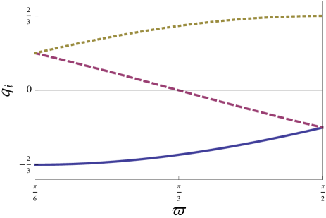
Figure 1: Evolution of $q_{i}$ with $\varpi$ ($q_{1}$ in solid line, $q_{2}$ in dashed line and $q_{3}$ in dotted line). We can choose $\varpi\in[\frac{\pi}{6},\frac{\pi}{2}]$ so that $p_{1}\leq p_{2}\leq p_{3}$.

It is thus clear that the spatial metric is explicitely given by

$$\gamma_{ij}(t)={\rm diag}\left[\left(\frac{t}{t_{0}}\right)^{2q_{i}}\right]\quad\hbox{with}\quad q_{i}=p_{i}-\frac{1}{3}$$ (6)

so that

$$\sum_{i}q_{i}=0,\qquad\sum_{i}q_{i}^{2}=\frac{2}{3}\,.$$ (7)

The $q_{i}$ are explicitely given by

$$q_{i}=\frac{2}{3}\sin\varpi_{i}.$$ (8)

We also define the useful parameterisation

$$Q_{i}\equiv\frac{3}{2}q_{i}=\sin\varpi_{i}$$ (9)

such that $Q_{i}\in[-1,1]$. We define the conformal time $\eta$ from ${\rm d}t\equiv S{\rm d}\eta$, and the metric (1) can then be recast as

$${\rm d}s^{2}=S^{2}(\eta)\left[-{\rm d}\eta^{2}+\gamma_{ij}(\eta){\rm d}x^{i}{\rm d}x^{j}\right].$$ (10)

From the previous analysis, we have $\eta=\frac{3}{2}t_{0}(t/t_{0})^{\frac{2}{3}}$ so that we set

$$S(\eta)=\sqrt{\frac{\eta}{\eta_{0}}}\quad\hbox{with}\quad\eta_{0}=\frac{3}{2}t_{0}$$ (11)

and also

$$t=\frac{2}{3}S\eta.$$ (12)

We easily deduce that

$$\gamma_{ij}={\rm diag}\left[\left(\frac{\eta}{\eta_{0}}\right)^{3q_{i}}\right],\quad\gamma^{ij}={\rm diag}\left[\left(\frac{\eta}{\eta_{0}}\right)^{-3q_{i}}\right].$$ (13)

We define the comoving Hubble parameter by $\mathcal{H}\equiv S^{\prime}/S$, where a prime refers to a derivative with respect to the conformal time so that

$$\mathcal{H}=SH=\frac{1}{2\eta}\,.$$ (14)

The shear tensor is defined as $\sigma_{ij}\equiv\frac{1}{2}\gamma_{ij}^{\prime}$ and is traceless ($\gamma^{ij}\sigma_{ij}\equiv\sigma^{i}_{i}=0$) so that

$$\Sigma_{ij}\equiv\frac{\sigma_{ij}}{\mathcal{H}}=3{\rm diag}\left[q_{i}\left(\frac{\eta}{\eta_{0}}\right)^{3q_{i}}\right]$$ (15)

and thus $\Sigma^{i}_{j}=3{\rm diag}[q_{i}]$ so that

$$\Sigma^{2}=6,\qquad 2S^{2}\mathcal{H}=\eta_{0}^{-1}$$ (16)

and the Einstein equations imply that the shear satisfies

$$\left(\sigma^{i}_{j}\right)^{\prime}+2\mathcal{H}\sigma^{i}_{j}=0.$$ (17)

We also define the shear in cosmic time by

$$\hat{\sigma}_{ij}\equiv\frac{1}{2}\frac{{\rm d}\gamma_{ij}}{{\rm d}t}=\frac{\sigma_{ij}}{S}\,.$$ (18)

II.2 Weyl Tensor

The Kasner spacetime is a vacuum solution of Einstein equations and this implies that

$$R_{\mu\nu}=0,\quad R=0,\quad R_{\mu\nu\rho\sigma}=C_{\mu\nu\rho\sigma}.$$ (19)

It is thus only characterized by its Weyl tensor, both at the background and perturbation level. The Weyl tensor has just two types of non-vanishing components which are the $C^{0i}_{\phantom{0i}0j}$ and the $C^{0i}_{\phantom{0i}jk}$. The former are related to the components of the type $C^{ij}_{\phantom{ij}kl}$ (thanks to the traceless conditions) and to the electric part of the Weyl tensor. The latter are related to its magnetic part, and it vanishes for the background Kasner spacetime. The only non-vanishing components of the background Weyl tensor are thus expressed as

$$C^{0i}_{\phantom{0i}0j} = -H\hat{\sigma}^{i}_{j}-\frac{1}{3}\hat{\sigma}^{2}\delta^{i}_{j}+\hat{\sigma}^{i}_{k}\hat{\sigma}^{k}_{j},$$ (20)

$$C^{ij}_{\phantom{ij}kl} = \frac{1}{3}\hat{\sigma}^{2}\gamma^{i}_{[k}\gamma_{l]}^{j}+2\hat{\sigma}^{i}_{[k}\hat{\sigma}_{l]}^{j}$$ (21)

$$+2H\left(\gamma^{i}_{[k}\hat{\sigma}_{l]}^{j}+\hat{\sigma}^{i}_{[k}\gamma_{l]}^{j}\right),$$

where $[ij]$ refers to the antisymmetrisation of indices such that for an antisymmetric tensor $X_{ij}=X_{[ij]}$ (and similarly later on, $(ij)$ refers to the symmetrisation of indices such that for a symmetric tensor $X_{ij}=X_{(ij)}$). These Weyl components are explicitely given by

$$C^{0i}_{\phantom{0i}0j} = -\frac{1}{3t^{2}}\left(q_{i}+\frac{2}{3}-3q_{i}^{2}\right)\delta^{i}_{j},$$ (22)

$$= -\frac{1}{t^{2}}p_{i}\left(1-p_{i}\right)\delta^{i}_{j},$$ (23)

$$C^{ij}_{\phantom{ij}kl} = \frac{2}{t^{2}}p_{i}p_{j}\delta^{i}_{[k}\delta_{l]}^{j},$$ (24)

and it is easy to notice explicitely that these two types of components are not independent and are related thanks to Eq. (170). We thus obtain that $C^{2}\equiv C_{\mu\nu\rho\sigma}C^{\mu\nu\rho\sigma}$ is given by

$$C^{2} = 12{\cal C}^{2}\sin^{2}\left(\frac{3\varpi}{2}+\frac{\pi}{4}\right)$$ (25)

$$= -3^{4}{\cal C}^{2}p_{1}p_{2}p_{3}$$

$$= 3^{4}{\cal C}^{2}p_{I}^{2}(1-p_{I})$$

$$= 3{\cal C}^{2}\left(1+3q_{I}\right)^{2}\left(2-3q_{I}\right)$$

$$= 6{\cal C}^{2}\left(1+2Q_{I}\right)^{2}\left(1-Q_{I}\right)$$

where in the last equalities, $I$ can take any of the values $1,2,3$. The function ${\cal C}^{2}$ is given by [using Eq. (12)]

$${\cal C}^{2}=\left(\frac{2}{3t}\right)^{4}=\frac{1}{(S\eta)^{4}}\,.$$ (26)

The Weyl tensor and his algebraic properties are used to classify spacetimes by their Petrov type. Defining the tracefree symmetric rank-2 tensor $Q_{ij}=-E_{ij}-{\rm i}H_{ij}$ in terms of the electric ($E_{ij}$) and magnetic ($H_{ij}$) parts of the Weyl tensor, provides a way to classify the Weyl tensors petrov . For a Kasner spacetime, since the magnetic part of the Weyl tensor vanishes we obtain

$$Q^{i}_{j}=-E^{i}_{j}=C^{0i}_{\phantom{0i}0j}=-\frac{1}{t^{2}}p_{i}\left(1-p_{i}\right)\delta^{i}_{j}.$$ (27)

The eigenvalues $\lambda_{i}$ of $Q^{i}_{j}$ define its Petrov type. They are all real and different so that a generic Kasner spacetime ($\varpi\not=\frac{\pi}{6},\frac{\pi}{2}$) has Petrov type I while the two axially symmetric solutions with degenerate eigenvalues are of type O when $\varpi=\frac{\pi}{2}$ and of type D when $\varpi=\frac{\pi}{6}$ petrov .

III Perturbation theory in a Kasner spacetime

The Kasner spacetime being a particular case of Bianchi universe, the study of the evolution of the perturbations derives simply from our previous formalism ppu1 ; ppu2 that we specialize to the vacuum, using that $S^{\prime\prime}/S=-1/(4\eta^{2})$ so that $\mathcal{H}^{\prime}=-2\mathcal{H}^{2}$ and the property (16).

III.1 Generalities

Following the formalism developed in Refs. ppu1 ; ppu2 , we consider the general metric of an almost Bianchi I spacetime,

$${\rm d}s^{2} = S^{2}\left[-\left(1+2A\right){\rm d}\eta^{2}+2\bar{B}_{i}{\rm d}x^{i}{\rm d}\eta\right.$$ (28)

$$\qquad\qquad\left.+\left(\gamma_{ij}+h_{ij}\right){\rm d}x^{i}{\rm d}x^{j}\right].$$

$\bar{B}_{i}$ and $h_{ij}$ can be further decomposed into scalar, vector and tensor components as

$$\bar{B}_{i} = \partial_{i}B+B_{i}\,,$$ (29)

$$h_{ij} \equiv 2C\left(\gamma_{ij}+\Sigma_{ij}\right)+2\partial_{i}\partial_{j}E+2\partial_{(i}E_{j)}+2\tilde{E}_{ij}\,,$$

with

$$\partial_{i}B^{i}=0=\partial_{i}E^{i},\quad\tilde{E}_{i}^{i}=0=\partial_{i}\tilde{E}^{ij}.$$ (30)

We then construct the gauge invariant quantities and define the conformal Newtonian gauge by the conditions

$$B=B^{i}=E=0\,,$$ (31)

so that

$$A=\Phi\,,\qquad C=-\Psi\,,\qquad\Phi^{i}=-(E^{i})^{\prime}\,.$$ (32)

We also introduce the extremely useful variable pubook

$$X\equiv\Phi+\Psi+\left(\frac{\Psi}{\mathcal{H}}\right)^{\prime}.$$ (33)

The tensor variable $\tilde{E}_{ij}$ is readily gauge invariant. At this stage, we are left with $10-4=6$ degrees of freedom: two scalars ($\Phi$ and $\Psi$), two vectors ($\Phi^{i}$) and two tensors ($\tilde{E}_{ij}$). Contrary to the perturbation theory around a spatially homogeneous and isotropic spacetime pubook , the three types of perturbations do not decouple.

As we shall now see, the perturbation equations will exhibit four constraints so that only two dynamical degrees of freedom related to the gravity waves remain, as in Minkowski or de Sitter spacetimes.

III.2 Mode decomposition

The perturbation equations are conveniently written in Fourier space and we decompose any quantity in Fourier modes as follows. Using the Cartesian comoving coordinates system $\{x^{i}\}$ on the constant time hypersurfaces, we decompose any scalar function as

$$f\left(x^{j},\eta\right)=\int\frac{{\rm d}^{3}k_{i}}{\left(2\pi\right)^{\frac{3}{2}}}\,f\left(k_{i},\eta\right)\,\hbox{e}^{\mathrm{i}k_{i}x^{i}}\,.$$ (34)

The comoving wave co-vectors $k_{i}$ are constant, $k_{i}^{\prime}=0$. We now define $k^{i}\equiv\gamma^{ij}k_{j}$ which is now time-dependent and explicitely given by

$$k^{i}=k_{i}\left(\frac{\eta}{\eta_{0}}\right)^{-2Q_{i}}$$ (35)

so that

$$k^{2}\equiv k_{i}k^{i}=\sum_{i}x_{i}^{2},\qquad x_{i}\equiv k_{i}\left(\frac{\eta}{\eta_{0}}\right)^{-Q_{i}}\,.$$ (36)

For any mode $k_{i}$, a basis $\{e_{1},e_{2}\}$ of the subspace perpendicular to $k_{i}$ can be constructed from the natural Cartesian basis as (see Appendix A of Ref. ppu2 for the details of the construction)

$$e^{i}_{1}=\left(\frac{\eta}{\eta_{0}}\right)^{-Q_{i}}\omega_{1}^{i},\qquad e^{i}_{2}=\left(\frac{\eta}{\eta_{0}}\right)^{-Q_{i}}\omega_{2}^{i}$$ (37)

with

$$\omega_{1}^{i}=\left(\begin{array}[]{c}\cos\gamma\cos\beta\cos\alpha-\sin\alpha\sin\gamma\\ \cos\gamma\sin\alpha+\cos\alpha\cos\beta\sin\gamma\\ -\cos\alpha\sin\beta\end{array}\right),$$ (38)

$$\omega_{2}^{i}=\left(\begin{array}[]{c}-\cos\gamma\cos\beta\sin\alpha-\cos\alpha\sin\gamma\\ \cos\gamma\cos\alpha-\sin\alpha\cos\beta\sin\gamma\\ \sin\alpha\sin\beta\end{array}\right).$$ (39)

The three Euler angles $(\alpha,\beta,\gamma)$ depend on time and are explicitely given by

$$\sin\gamma\sin\beta=\frac{x_{2}}{k},\quad\cos\gamma\sin\beta=\frac{x_{1}}{k}$$ (40)

so that $\tan\gamma=x_{2}/x_{1}=(k_{2}/k_{1})(\eta/\eta_{0})^{(Q_{1}-Q_{2})}$ and

$$\cos\beta=\frac{x_{3}}{k}\,.$$ (41)

The previous relations determine $\beta(\eta)$ and $\gamma(\eta)$. The requirement that $\{e_{1},e_{2}\}$ remains orthogonal to $k_{i}$ imposes that

$$\alpha^{\prime}=-\cos\beta\gamma^{\prime},$$ (42)

which can be rewritten as

$$\alpha^{\prime}=\frac{(Q_{2}-Q_{1})}{\eta}\frac{x_{3}}{k}\frac{1}{\frac{x_{1}}{x_{2}}+\frac{x_{2}}{x_{1}}}\,,$$ (43)

which determines $\alpha(\eta)$ up to an integration constant.

The vector and tensor modes can then be decomposed respectively as

$$\Phi_{i}(k_{i},\eta)=\sum_{a=1,2}\Phi_{a}(k_{i},\eta)\,e_{i}^{a}(\hat{k}_{i})\,,$$ (44)

and

$$\tilde{E}_{ij}(k_{i},\eta)=\sum_{\lambda=+,\times}E_{\lambda}(k_{i},\eta)\,\varepsilon_{ij}^{\lambda}(\hat{k}_{i})$$ (45)

where the polarisation tensors have been defined as

$$\varepsilon_{ij}^{\lambda}\equiv\frac{e_{i}^{1}e_{j}^{1}-e_{i}^{2}e_{j}^{2}}{\sqrt{2}}\delta^{\lambda}_{+}+\frac{e_{i}^{1}e_{j}^{2}+e_{i}^{2}e_{j}^{1}}{\sqrt{2}}\delta^{\lambda}_{\times}.$$ (46)

III.3 Shear components

The perturbation equations in Fourier space involve the components of the decomposition of the shear on the basis $\{\hat{k},e_{1},e_{2}\}$. Since it is a symmetric trace-free tensor, it can be decomposed as

$$\sigma_{ij} = \frac{3}{2}\left(\hat{k}_{i}\hat{k}_{j}-\frac{1}{3}\gamma_{ij}\right)\sigma_{{}_{\parallel}}+2\sum_{a=1,2}\sigma_{{}_{\rm V}a}\,\hat{k}_{(i}e^{a}_{j)}$$ (47)

$$+\sum_{\lambda=+,\times}\sigma_{{}_{\rm T}\lambda}\,\varepsilon^{\lambda}_{ij}\,.$$

This decomposition involves 5 independent components of the shear in a basis adapted to the wavenumber $k_{i}$. We must stress however that $(\sigma_{{}_{\parallel}},\sigma_{{}_{\rm V}a},\sigma_{{}_{\rm T}\lambda})$ must not be interpreted as the Fourier components of the shear, even if they explicitely depend on $k_{i}$. This dependence arises from the local anisotropy of space. A similar decompositon for $\Sigma_{ij}$ defines the coefficients $(\Sigma_{{}_{\parallel}},\Sigma_{{}_{\rm V}a},\Sigma_{{}_{\rm T}\lambda})$ and we obtain from Einstein equation in vacuum that it must satisfy the constraint

$$6=\Sigma^{2}\equiv\frac{\sigma_{ij}\sigma^{ij}}{\mathcal{H}^{2}}=\frac{3}{2}\Sigma_{{}_{\parallel}}^{2}+2\sum_{a}\Sigma_{{}_{\rm V}a}^{2}+\sum_{\lambda}\Sigma_{{}_{\rm T}\lambda}^{2}\,,$$ (48)

which is independent of $k_{i}$.

The equation of evolution of the shear (17) implies that

$$\Sigma_{{}_{\parallel}}^{\prime}=-2\mathcal{H}\sum_{a}\Sigma_{{}_{\rm V}a}^{2}$$ (49)

$$\Sigma_{{}_{\rm V}a}^{\prime}=\mathcal{H}\left(\frac{3}{2}\Sigma_{{}_{\rm V}a}\Sigma_{{}_{\parallel}}-\sum_{b,\lambda}\Sigma_{{}_{\rm V}b}\Sigma_{{}_{\rm T}\lambda}\mathcal{M}_{ab}^{\lambda}\right),$$ (50)

$$\Sigma_{{}_{\rm T}\lambda}^{\prime}=2\mathcal{H}\sum_{a,b}\mathcal{M}_{ab}^{\lambda}\Sigma_{{}_{\rm V}a}\Sigma_{{}_{\rm V}b}\,,$$ (51)

where the matrix $\mathcal{M}_{ab}^{\lambda}$ is defined by

$${\cal M}_{ab}^{\lambda}=\frac{1}{\sqrt{2}}\left(\begin{array}[]{cc}1&0\\ 0&-1\end{array}\right)\delta^{\lambda}_{+}+\frac{1}{\sqrt{2}}\left(\begin{array}[]{cc}0&1\\ 1&0\end{array}\right)\delta^{\lambda}_{\times}\,.$$ (52)

The equation (47) can be inverted to get

$$\Sigma_{{}_{\parallel}} = 2\sum_{i}Q_{i}\frac{x_{i}^{2}}{k^{2}},$$ (53)

$$\Sigma_{{}_{\rm V}a} = 2\sum_{i}Q_{i}\frac{x_{i}}{k}\omega^{i}_{a},$$ (54)

$$\Sigma_{{}_{\rm T}\lambda} = 2\sum_{i}Q_{i}\left(\frac{\eta}{\eta_{0}}\right)^{2Q_{i}}\varepsilon_{\lambda}^{ii}.$$ (55)

The last equation implies, using Eq. (46), that

$$\Sigma_{{}_{\rm T}+} = \sqrt{2}\sum_{i}Q_{i}\left[(\omega_{1}^{i})^{2}-(\omega_{2}^{i})^{2}\right]$$ (56)

$$\Sigma_{{}_{\rm T}\times} = 2\sqrt{2}\sum_{i}Q_{i}\omega_{1}^{i}\omega_{2}^{i}.$$ (57)

III.4 Perturbation equations

We use the equations derived in Refs. ppu1 ; ppu2 when applied to the particular case of a vacuum solution (so that $v\rightarrow 0$).

The two scalar perturbations are explicitely obtained from the tensor modes as

$$X=\frac{1}{2-\Sigma_{{}_{\parallel}}}\sum_{\lambda}\Sigma_{{}_{\rm T}\lambda}E_{\lambda}\,.$$ (58)

We then deduce that $\Psi$ is given by

$$k^{2}\Psi = -\mathcal{H}X^{\prime}$$

$$-\frac{4\mathcal{H}^{2}}{2-\Sigma_{{}_{\parallel}}}\left(\sum_{a}\Sigma_{{}_{\rm V}a}^{2}X-\sum_{a,b,\lambda}{\cal M}^{\lambda}_{ab}\Sigma_{{}_{\rm V}a}\Sigma_{{}_{\rm V}b}E_{\lambda}\right),$$

while the second Bardeen potential is then given by

$$k^{2}\Phi=k^{2}\left(4-\Sigma_{{}_{\parallel}}\right)\Psi+3\mathcal{H}X^{\prime}.$$ (60)

The vector mode is then given by

$$\Phi_{a}=-2\mathrm{i}\frac{\mathcal{H}}{k}\sum_{\lambda}\left[2\sum_{b}{\cal M}_{ab}^{\lambda}\Sigma_{{}_{\rm V}b}-\Sigma_{{}_{\rm T}\lambda}\frac{{\Sigma}_{{}_{\rm V}a}}{2-\Sigma_{{}_{\parallel}}}\right]E_{\lambda}.$$ (61)

This shows that the scalar and vector modes are obtained algebraically from the tensor modes, which are the only degrees of freedom that propagate. Using the shorthand notation $(1-\lambda)$ for the opposite polarisation of $\lambda$, i.e. meaning that if $\lambda=+$, then $(1-\lambda)=\times$, and vice-versa, and introducing

$$\mu_{\lambda}\equiv SE_{\lambda},$$ (62)

we have

$$\mu_{\lambda}^{\prime\prime}+\left(k^{2}+\frac{1}{4\eta^{2}}\right)\mu_{\lambda} = 2\mathcal{H}^{2}\left(\Sigma_{{}_{\rm T}(1-\lambda)}^{2}\mu_{\lambda}-\Sigma_{{}_{\rm T}+}\Sigma_{{}_{\rm T}\times}\mu_{\left(1-\lambda\right)}\right)+2\mathcal{H}\sum_{\nu}\left(\frac{\Sigma_{{}_{\rm T}\nu}\Sigma_{{}_{\rm T}\lambda}}{2-\Sigma_{{}_{\parallel}}}\right)^{\prime}\mu_{\nu}+\mathcal{H}\Sigma_{{}_{\parallel}}^{\prime}\mu_{\lambda}.$$ (63)

The general solution of this linear equation can always be obtained in terms of four transfer functions as

$$E_{\lambda}(k_{i},\eta)=T^{\uparrow}_{\lambda\lambda^{\prime}}(k_{i},\eta)a_{\lambda^{\prime}}(k_{i},\eta_{0})+T^{\downarrow}_{\lambda\lambda^{\prime}}(k_{i},\eta)b_{\lambda^{\prime}}(k_{i},\eta_{0}),$$ (64)

where $a_{\lambda^{\prime}}(k_{i},\eta_{0})$ and $b_{\lambda^{\prime}}(k_{i},\eta_{0})$ are the initial conditions. The notations $\downarrow$ and $\uparrow$ refer respectively to a decaying and a growing mode. When the two polarisations are decoupled (which is the case asymptotically at early and late times, as we whall see below) then we only have two transfer functions to consider $T^{\uparrow}_{\lambda\lambda^{\prime}}=T^{\uparrow}_{\lambda}\delta_{\lambda\lambda^{\prime}}$ and $T^{\uparrow}_{\lambda\lambda^{\prime}}=T^{\downarrow}_{\lambda}\delta_{\lambda\lambda^{\prime}}$ since the transfer of power from one polarisation to the other is negligible. Similarly we define transfer functions for $\Psi$, $X$ and $\Phi_{a}$ by

$$\Psi(k_{i},\eta)=T^{\uparrow}_{\Psi,\lambda}(k_{i},\eta)a_{\lambda}(k_{i},\eta_{0})+T^{\downarrow}_{\Psi,\lambda}(k_{i},\eta)b_{\lambda}(k_{i},\eta_{0}),$$ (65)

$$X(k_{i},\eta)=T^{\uparrow}_{X,\lambda}(k_{i},\eta)a_{\lambda}(k_{i},\eta_{0})+T^{\downarrow}_{X,\lambda}(k_{i},\eta)b_{\lambda}(k_{i},\eta_{0}),$$ (66)

$$\Phi_{a}(k_{i},\eta)=T^{\uparrow}_{\Phi_{a},\lambda}(k_{i},\eta)a_{\lambda}(k_{i},\eta_{0})+T^{\downarrow}_{\Phi_{a},\lambda}(k_{i},\eta)b_{\lambda}(k_{i},\eta_{0}).$$ (67)

III.5 Summary

In conclusion, for a given model, one can determine $(\Sigma_{{}_{\parallel}},\Sigma_{{}_{\rm V}a},\Sigma_{{}_{\rm T}\lambda})$ for each mode $k_{i}$ and then solve Eq. (63) for the gravitational waves. One can then deduce $\Phi$, $\Psi$ and $\Phi_{a}$ algebraically. As expected, only two degrees of freedom can propagate. The existence of the vector and tensor modes arises from the fact that isotropy is violated so that the SVT modes do not decouple. The Kasner case, being a vacuum solution, is thus simpler than the Bianchi I case studied in Refs. ppu1 ; ppu2 .

IV Stability analysis

IV.1 Generalities

In full generality, the stability analysis requires first to solve Eq. (63) to determine the four transfer functions defined in Eq. (64). This allows to evaluate the effect of the perturbations on the square of the Weyl tensor, which is by construction independent of the choices of gauge and coordinates system. We thus introduce

$$\Xi\equiv\frac{C^{2}}{\bar{C}^{2}}$$ (68)

where $\bar{C}^{2}$ is the background value of $C^{2}$ given in Eq. (25) such that at the background level $\bar{\Xi}=1$, and at the perturbed level up to second order we have when $\bar{C}^{2}\neq 0$

$$\delta^{(1)}C^{2} = \bar{C}^{2}\Xi^{(1)}\,,$$ (69)

$$\delta^{(2)}C^{2} = \bar{C}^{2}\Xi^{(2)}\,.$$ (70)

The perturbation of $\Xi$ at first order in the perturbations, $\Xi^{(1)}({\bf x},\eta)$, can be decomposed in Fourier modes as

$$\Xi^{(1)}({\bf x},\eta)=\int\frac{{\rm d}^{3}{\bf k}}{(2\pi)^{\frac{3}{2}}}\Xi^{(1)}({\bf k},\eta)\hbox{e}^{{\rm i}{\bf k}.{\bf x}}.$$ (71)

In order to assess the behaviour of $C^{2}$ at early and late time, we assume that at an arbitrary initial time $\eta_{0}$ the initial conditions for the two modes defined in Eq. (64) are such that (1) they are not correlated,

$$\langle a_{\lambda}({\bf k})b_{\lambda^{\prime}}^{\star}({\bf k}^{\prime})\rangle=0,$$ (72)

and that (2) they have the same initial power spectrum,

$$\langle a_{\lambda}({\bf k})a_{\lambda^{\prime}}^{\star}({\bf k}^{\prime})\rangle=\delta^{3}({\bf k}-{\bf k}^{\prime})\delta_{\lambda\lambda^{\prime}}P_{\rm init}(k_{i}),$$ (73)

$$\langle b_{\lambda}({\bf k})b_{\lambda^{\prime}}^{\star}({\bf k}^{\prime})\rangle=\delta^{3}({\bf k}-{\bf k}^{\prime})\delta_{\lambda\lambda^{\prime}}P_{\rm init}(k_{i}).$$ (74)

The initial power spectrum is an unknown function of the comoving wave-vector $k_{i}$. It is clear that

$$\langle\Xi^{(1)}({\bf x},\eta)\rangle=0$$ (75)

at all time. This is indeed not the case for the perturbation of $\Xi$ at second order in perturbations, $\Xi^{(2)}({\bf x},\eta)$, since it is quadratic. The previous definitions allow to compute that at lowest order $\langle\Xi({\bf x},\eta)\rangle=\langle\Xi^{(2)}({\bf x},\eta)\rangle$ with

$$\langle\Xi^{(2)}({\bf x},\eta)\rangle=\int\frac{{\rm d}^{3}{\bf k}}{(2\pi)^{3}}P_{\rm init}(k_{i})\sum_{\lambda}\Xi^{(2)}_{\lambda}(\bf k,\eta)$$ (76)

and we define

$$\Xi^{(2)}({\bf k},\eta)\equiv\sum_{\lambda}\Xi^{(2)}_{\lambda}({\bf k},\eta).$$ (77)

The function $\Xi^{(2)}_{\lambda}(\bf k,\eta)$ can in principle be expressed in terms of the transfer functions that appear in Eq. (64) and in terms of the coefficients $\Sigma_{\parallel}({\bf k},\eta)$…

From a numerical point of view, the situation is thus clear but very time consuming. It is also unnecessary to solve the evolution equations in their full generality since we are interested in the asymptotic behaviour of $\langle\Xi^{(2)}({\bf x},\eta)\rangle$ when $\eta/\eta_{0}\rightarrow+\infty$ or $\eta/\eta_{0}\rightarrow 0$. In these two regimes, the wave numbers tend to focus along a principal axis since [see Eq. (36)]

$$k\rightarrow k_{1}\left(\frac{\eta}{\eta_{0}}\right)^{-Q_{1}},\qquad\frac{\eta}{\eta_{0}}\rightarrow+\infty$$ (78)

and

$$k\rightarrow k_{3}\left(\frac{\eta}{\eta_{0}}\right)^{-Q_{3}},\qquad\frac{\eta}{\eta_{0}}\rightarrow 0.$$ (79)

We shall thus discuss the dynamics of the perturbations when their mode is aligned along a principal axis (§ IV.2) and their contribution to $\Xi^{(2)}_{\lambda}(\bf k,\eta)$ (§ IV.3). These two steps can be performed completely analytically so that we can then discuss the general behaviour of $\langle\Xi^{(2)}({\bf x},\eta)\rangle$ at late time (§ IV.4) and early time (§ IV.5).

IV.2 Dynamics of the perturbation for modes aligned along a principal axis

IV.2.1 General behaviour

We assume that only one of the components of the Fourier space, indexed by $I$, satisfies $k_{I}\not=0$. It is then clear that $k^{2}=k_{I}^{2}(\eta/\eta_{0})^{-2Q_{I}}$ so that

$$\Sigma_{{}_{\parallel}}=2Q_{I}.$$ (80)

Then, since $\Sigma_{{}_{\parallel}}^{\prime}=0$, we conclude from Eq. (49) that $\sum_{a}\Sigma_{{}_{\rm V}a}^{2}=0$ because of Eq. (50) and thus

$$\Sigma_{{}_{\rm V}a}=0.$$ (81)

This implies, from Eq. (61), that

$$\Phi_{a}=0.$$ (82)

It follows from Eq. (51) that $\Sigma_{{}_{\rm T}\lambda}^{\prime}=0$, and it can be checked that

$$\left|\Sigma_{{}_{\rm T}+}\right|=\frac{3}{\sqrt{2}}\Delta_{I},\qquad\Sigma_{{}_{\rm T}\times}=0$$ (83)

where we have defined

$$\Delta_{I}\equiv q_{{\rm max}(i\not=I)}-q_{{\rm min}(i\not=I)}$$ (84)

which is explicitely given by

$$\Delta_{I}=\frac{2}{\sqrt{3}}\left|\cos\varpi_{I}\right|=\sqrt{\frac{4}{3}-3q_{I}^{2}}=2\sqrt{\frac{(1-Q_{I}^{2})}{3}}.$$ (85)

The scalar perturbations are then given algebraically by

$$X=\frac{\Sigma_{{}_{\rm T}+}}{2-3q_{I}}E_{+}=\frac{\Sigma_{{}_{\rm T}+}}{2(1-Q_{I})}E_{+}$$ (86)

that derives from Eq. (58) from which we deduce that Eqs. (III.4-60) reduce to

$$k^{2}\Psi = -\mathcal{H}X^{\prime},\qquad k^{2}\Phi=-(1-2Q_{I})\mathcal{H}X^{\prime}.$$ (87)

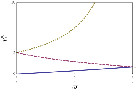
Figure 2: Evolution of the index of the Bessel function, $\nu^{\times}_{i}$, with $\varpi$ ($\nu^{\times}_{1}$ in solid line, $\nu^{\times}_{2}$ in dashed line and $\nu^{\times}_{3}$ in dotted line). We recall that $\nu^{+}_{i}=0$ whatever $\varpi$.

The only equations to solve are Eqs. (63) for the gravity. They decouple for each polarisation and lead to the system

$$\mu_{+}^{\prime\prime}+\left[k_{I}^{2}\left(\frac{\eta}{\eta_{0}}\right)^{-2Q_{I}}+\frac{1}{4\eta^{2}}\right]\mu_{+}=0,$$ (88)

$$\mu_{\times}^{\prime\prime}+\left[k_{I}^{2}\left(\frac{\eta}{\eta_{0}}\right)^{-2Q_{I}}+\frac{1-9\Delta_{I}^{2}}{4\eta^{2}}\right]\mu_{\times}=0.$$ (89)

These two equations are compatible with the general equations (138-140) obtained for $\varpi=\frac{\pi}{6}$ and, in this particular case, with those derived in Ref. emir . The general solutions of Eqs. (88-89) can both be obtained as [see Eqs. (193-194)] the linear combination (64) with

$$T^{\uparrow}_{\lambda}(k_{I},\eta)={\cal J}^{\lambda}_{\nu_{I}}(k_{I},\eta),\quad T^{\downarrow}_{\lambda}(k_{I},\eta)={\cal N}^{\lambda}_{\nu_{I}}(k_{I},\eta)$$ (90)

where

$${\cal J}^{\lambda}_{I}(k_{I},\eta) = J_{\nu_{I}^{\lambda}}\left[\frac{k_{I}\eta_{0}}{1-Q_{I}}\left(\frac{\eta}{\eta_{0}}\right)^{1-Q_{I}}\right],$$ (91)

$${\cal N}^{\lambda}_{I}(k_{I},\eta) = N_{\nu_{I}^{\lambda}}\left[\frac{k_{I}\eta_{0}}{1-Q_{I}}\left(\frac{\eta}{\eta_{0}}\right)^{1-Q_{I}}\right].$$ (92)

Here, $J_{\nu_{I}^{\lambda}}$ and $N_{\nu_{I}^{\lambda}}$ are the Bessel and Newmann functions of index

$$\nu_{I}^{\times}\equiv\frac{3\Delta_{I}}{2(1-Q_{I})}=\sqrt{\frac{3(1+Q_{I})}{(1-Q_{I})}}\,,\qquad\nu_{I}^{+}=0,$$ (93)

and $\nu_{I}^{\times}$ is depicted on Fig. 2 (note that $\nu_{I}^{\times}$ is always non-negative while $\Sigma_{{}_{\rm T}+}$ can be negative). It is then clear that

$$|X|=\nu_{I}^{\times}\frac{E_{+}}{\sqrt{2}}$$ (94)

so that the two Bardeen potentials are given by

$$\Psi = -\frac{1}{k_{I}^{2}\eta_{0}^{2}}\left(\frac{\eta}{\eta_{0}}\right)^{-2(1-Q_{I})}\frac{\Sigma_{{}_{\rm T}+}}{4(1-Q_{I})}\frac{\partial E_{+}}{\partial\ln\frac{\eta}{\eta_{0}}}$$ (95)

$$\Phi = (1-2Q_{I})\Psi.$$ (96)

If follows that for these particular modes, the solution of the dynamics is obtained completely analytically. Figures 3 give an example of the behaviour of the tensor and scalar modes.

IV.2.2 Late time behaviour

The late time behaviour of the perturbations can be easily understood using the large argument expansions (195) and (197) of the Bessel functions, since

$$T^{\uparrow}_{\lambda} \simeq \sqrt{\frac{2}{\pi\ell_{1}}}\left(\frac{\eta}{\eta_{0}}\right)^{-\frac{1-Q_{1}}{2}}\cos\left[\ell_{1}\left(\frac{\eta}{\eta_{0}}\right)^{1-Q_{1}}\!\!\!\!\!\!-\nu_{1}\frac{\pi}{2}-\frac{\pi}{4}\right]$$

$$T^{\downarrow}_{\lambda} \simeq \sqrt{\frac{2}{\pi\ell_{1}}}\left(\frac{\eta}{\eta_{0}}\right)^{-\frac{1-Q_{1}}{2}}\sin\left[\ell_{1}\left(\frac{\eta}{\eta_{0}}\right)^{1-Q_{1}}\!\!\!\!\!\!-\nu_{1}\frac{\pi}{2}-\frac{\pi}{4}\right]$$

with

$$\ell_{1}=\frac{2k_{1}\eta_{0}}{2-3q_{1}}=\frac{k_{1}\eta_{0}}{1-Q_{1}}\,.$$ (97)

It follows that the late time behaviour is in general of the form

$$E_{\lambda}\sim\sqrt{\frac{2}{\pi\ell_{1}}}\left(\frac{\eta}{\eta_{0}}\right)^{-\frac{1-Q_{1}}{2}}A^{(\infty)}_{\lambda}\cos\left[\ell_{1}\left(\frac{\eta}{\eta_{0}}\right)^{1-Q_{1}}\!\!\!\!\!\!+\varphi^{(\infty)}_{\lambda}\right],$$ (98)

where $A^{(\infty)}_{\lambda}$ and $\varphi^{(\infty)}_{\lambda}$ are two constants that can easily be obtained in terms of $a_{\lambda}$ and $b_{\lambda}$. $X$ is then proportional to $E_{+}$ [see Eq. (94)] and $\Phi_{a}=0$, which completely determines the solution [see Eqs. (95-96)].

Figure 3: Evolution of $T_{\times}^{\uparrow}$ (left), $T_{+}^{\uparrow}$ (middle) and $T_{\Psi,+}^{\uparrow}$ (right) for a Kasner universe with $\varpi=\frac{\pi}{3}$, i.e. with $\{q_{i}\}=(-1/\sqrt{3},0,1/\sqrt{3})$) for the modes aligned with the axis 1 (dotted), 2 (dashed) and 3 (solid), assuming that $k_{I}\eta_{0}=1$.

IV.2.3 Early time behaviour

Asymptotically, the dominant term of the wavevector is aligned along the direction expanding the fastest, i.e $i=3$. The two polarisations behave differently because $\Delta_{3}\not=0$. Using the small argument expansions (196) and (199) of the Bessel function, we obtain that, since $1-Q_{3}\geq 0$, when $\eta\rightarrow 0$

$$T^{\uparrow}_{\times} \sim \frac{1}{\Gamma(1+\nu^{\times}_{3})}\left[\frac{\ell_{3}}{2}\left(\frac{\eta}{\eta_{0}}\right)^{1-Q_{3}}\right]^{\nu_{3}^{\times}}$$

$$T^{\downarrow}_{\times} \sim \frac{\Gamma(\nu_{3}^{\times})}{\pi}\left[\frac{\ell_{3}}{2}\left(\frac{\eta}{\eta_{0}}\right)^{1-Q_{3}}\right]^{-\nu_{3}^{\times}}$$ (99)

with

$$\ell_{3}=\frac{k_{3}\eta_{0}}{1-Q_{3}}\,.$$ (100)

These expressions hold as long as $Q_{3}\not=1$, that is for $\varpi\not=\frac{\pi}{2}$, a particular case that is discussed in Appendix B. The transfer functions for the $+$ polarisation behave as

$$T^{\uparrow}_{+} \sim \left[1-\left(\frac{\ell_{3}}{2}\right)^{2}\left(\frac{\eta}{\eta_{0}}\right)^{2(1-Q_{3})}\right]$$ (101)

$$T^{\downarrow}_{+} \sim \frac{2}{\pi}\left[\ln\left(\frac{\ell_{3}}{2}\left(\frac{\eta}{\eta_{0}}\right)^{1-Q_{3}}\right)+\gamma_{E}\right].$$ (102)

IV.3 Weyl tensor evolution for modes aligned along a principal axis

For these modes, the expressions of $\Xi^{(1)}_{\lambda}(\bf k,\eta)$ and $\Xi^{(2)}_{\lambda}(\bf k,\eta)$ turn out to simplify greatly and can be expressed in terms of the dimensionless parameter

$$x\equiv k\eta=x_{I}\eta\,.$$ (103)

First, $\Xi^{(1)}_{\lambda}(\bf k,\eta)$ can be expressed in terms of the two transfer functions and their first derivatives as

$$\Xi^{(1)}(k_{I},\eta)=\frac{1}{2(1-Q_{I})(1+2Q_{I})x^{2}}\sum_{i=0,1}f_{+}^{(i)}\frac{\partial^{i}T_{+}}{\partial(\ln\eta)^{i}}\,.$$

The two coefficients $f_{+}^{(i)}$ can be computed and are given by

$$f_{+}^{(0)} = \sqrt{2}\Delta_{I}[-6(1+2Q_{I})x^{2}+2x^{4}],$$ (104)

$$f_{+}^{(1)} = \sqrt{2}\Delta_{I}[-9(1+2Q_{I})+(7+2Q_{I})x^{2}].$$ (105)

Interestingly, the $\times$ polarisation does not contribute. In the above expression $T_{+}$ stands either for $T_{+}^{\downarrow}$ or $T_{+}^{\uparrow}$ depending on the solution (decaying, growing, or any linear combination of them) that is considered. When $\Delta_{I}=0$, $\Xi^{(1)}$ vanishes identically and, again, since $\langle\Xi^{(1)}\rangle=0$ we shall not consider this linear part any further.

The second order $\Xi^{(2)}$ can be expanded as

$$\Xi^{(2)}_{\lambda}(k_{I},\eta) = \frac{1}{6(1+2Q_{I})^{2}(1-Q_{I})}$$

$$\times\sum_{i=0,1}\sum_{j=0,1}f_{\lambda}^{(i,j)}\frac{\partial^{i}T_{\lambda}}{\partial(\ln\eta)^{i}}\frac{\partial^{j}T_{\lambda}}{\partial(\ln\eta)^{j}}$$

with the same conventions as for $\Xi^{(1)}$. The eight coefficients $f_{\lambda}^{(i,j)}$ are explicitely given by

$$f_{+}^{(0,0)} = 3(1+2Q_{I})^{2}(13+8Q_{I})(1+Q_{I})$$ (107)

$$\qquad+6x^{2}(-1+4Q_{I}^{2})+8x^{4}$$

$$f_{\times}^{(0,0)} = 6(1+2Q_{I})^{2}(1-Q_{I}^{2})+18x^{2}+8x^{4},$$ (108)

$$f_{+}^{(0,1)} = f_{+}^{(1,0)}$$ (109)

$$= \frac{1}{x^{2}}\left[3(1+2Q_{I})^{2}(1+Q_{I})(22+25Q_{I}-2Q_{I}^{2})\right.$$

$$+2(1+2Q_{I})(-26-29Q_{I}+Q_{I}^{2})x^{2}$$

$$\left.+4(1-Q_{I})x^{4}\right]$$

$$f_{\times}^{(0,1)} = f_{\times}^{(1,0)}$$ (110)

$$= -4(1-Q_{I})[(1+2Q_{I})^{2}-x^{2}]$$

and

$$f_{+}^{(1,1)} = x^{-4}\left[9(1+2Q_{I})^{2}(1+Q_{I})(3+2Q_{I}+4Q_{I}^{2})\right.$$

$$\qquad\times(5-2Q_{I})+2(13+4Q_{I}-8Q_{I}^{2})x^{4}+8x^{6}$$

$$\left.+9(1+2Q_{I})(1+Q_{I})(-17-18Q_{I}+8Q_{I}^{2})x^{2}\right]$$

$$f_{\times}^{(1,1)} = 2[(1+2Q_{I})^{2}+4x^{2}].$$ (111)

IV.4 Asymptotic behaviour at late times

At late time ($\eta\to\infty$), only the growing mode dominates and we can safely neglect the decaying mode since it would only lead to a redefinition of the phase $\varphi_{\infty}$; see Eq. (98). As can be concluded from the evolution (78) of the wave number, the parameter $x$ defined in Eq. (103) behaves as

$$x\to k_{1}\eta_{0}\left(\frac{\eta}{\eta_{0}}\right)^{1-Q_{1}}$$ (112)

which is always a growing function of $\eta$ (remember $q_{1}<0$ and thus $Q_{1}<0$; see Fig. 1). We thus need to take the limit when $x\to\infty$ of the transfer functions $T^{\uparrow}_{\lambda}$ and of their derivatives. From Eq. (98), we conclude that

$$T^{\uparrow}_{\lambda}\simeq\sqrt{\frac{2(1-Q_{1})}{\pi x}}\cos\left[\frac{x}{1-Q_{1}}\right].$$ (113)

Since

$$\frac{\partial x}{\partial\ln\eta}=\left(1-Q_{1}\right)x,$$ (114)

it implies that, at leading order in $x$,

$$\frac{\partial T^{\uparrow}_{\lambda}}{\partial\ln\eta}\simeq-\sqrt{\frac{2x(1-Q_{1})}{\pi}}\sin\left[\frac{x}{1-Q_{1}}\right].$$ (115)

Using the expansion (IV.3), we conclude that

$$\Xi^{(2)}_{\lambda}({\bf k},\eta) \to \frac{4x^{2}}{3}\frac{\left[\left({\frac{\partial T^{\uparrow}_{\lambda}}{\partial\ln\eta}}\right)^{2}+x^{2}{T^{\uparrow}_{\lambda}}^{2}\right]}{(1+2Q_{1})^{2}(1-Q_{1})}$$ (116)

$$\to \frac{8x^{3}}{3\pi(1+2Q_{1})^{2}}\,.$$

This expression is valid for any Kasner spacetime but for the particular case $\varpi=\frac{\pi}{2}$ that is discussed in Appendix B (since in that case $Q_{1}=-\frac{1}{2}$).

It follows that

$$\Xi^{(2)}_{\lambda}({\bf k},\eta)\propto x^{3}\propto\eta^{3(1-Q_{1})},$$ (117)

which is unbounded at late time.

IV.5 Asymptotic behaviour at early times

As can be concluded from the evolution (79) of the wave number, the parameter $x$ defined in Eq. (103) behaves, when $\eta\to 0$, as

$$x\to k_{3}\eta_{0}\left(\frac{\eta}{\eta_{0}}\right)^{1-Q_{3}}$$ (118)

which is always a decreasing function of $\eta$ (except if $\varpi=\frac{\pi}{2}$, see Appendix B for that particular case). It follows that we need to evaluate the limit $x\to 0$ of the transfer functions.

At early time, one can however not disregard the decaying mode since it diverges faster when $\eta\rightarrow 0$. The expression (IV.3) behaves as

$$\Xi^{(2)}({\bf k},\eta)\to\frac{(1+Q_{3})}{2(1-Q_{3})}(13+8Q_{3})T_{+}T_{+}$$ (119)

$$+\frac{(1+Q_{3})}{(1-Q_{3})x^{2}}(22+25Q_{3}-2Q_{3}^{2})T_{+}\frac{\partial T_{+}}{\partial\ln\eta}$$

$$+\frac{3(1+Q_{3})}{2(1-Q_{3})x^{4}}(5-2Q_{I})(3+2Q_{3}+4Q_{3}^{2})\left(\frac{\partial T_{+}}{\partial\ln\eta}\right)^{2}$$

$$+(1+Q_{3})T_{\times}T_{\times}-\frac{4}{3}T_{\times}\frac{\partial T_{\times}}{\partial\ln\eta}+\frac{1}{3(1-Q_{3})}\left(\frac{\partial T_{\times}}{\partial\ln\eta}\right)^{2}.$$

In order to determine the behaviour of the transfer functions, we consider two cases.

First, if we consider only the growing mode [i.e. $a_{\lambda}\neq 0$ and $b_{\lambda}=0$ in Eq. (64)] then we deduce from the expressions (99) and (102) of the transfer functions that

$${\frac{\partial T^{\uparrow}_{\times}}{\partial\ln\eta}} \simeq \frac{3}{2}\Delta_{3}T^{\uparrow}_{\times}\,,$$

$${\frac{\partial T^{\uparrow}_{+}}{\partial\ln\eta}} \simeq -\frac{x^{2}}{2(1-Q_{3})}T^{\uparrow}_{+}.$$ (120)

At leading order, the contributions of the two polarisations to $\Xi^{(2)}$ are thus

$$\Xi^{(2)}_{+}(k_{I},\eta) \to \frac{9(1-4Q_{3})^{2}(1+Q_{3})}{8(1-Q_{3})^{3}}{T_{+}^{\uparrow}}^{2}\,,$$

$$\Xi^{(2)}_{\times}(k_{I},\eta) \to 2(1+Q_{3}-\Delta_{3}){T^{\uparrow}_{\times}}^{2}.$$ (121)

Eqs. (99) and (102) tells that $T^{\uparrow}_{\times}\sim x^{\nu_{3}^{\times}}$ and $T^{\uparrow}_{+}\sim x^{0}$ so that $\Xi^{(2)}_{\times}(k_{I},\eta)\to 0$ (since $\nu_{3}^{\times}>0$) and $\Xi^{(2)}_{+}(k_{I},\eta)\to{\rm const.}$ Thus, the contribution of the growing mode leads to a bounded contribution to $\Xi^{(2)}$.

On the other hand, if we consider the decaying mode [i.e. $a_{\lambda}=0$ and $b_{\lambda}\not=0$ in Eq. (64)], i.e. the most diverging mode when $x\rightarrow 0$, then

$${\frac{\partial T^{\downarrow}_{\times}}{\partial\ln\eta}} \simeq -\frac{3}{2}\Delta_{3}T^{\downarrow}_{\times}$$

$${\frac{\partial T^{\downarrow}_{+}}{\partial\ln\eta}} \simeq \frac{2(1-Q_{3})}{\pi}\gg x^{2}T^{\downarrow}_{+}.$$ (122)

We conclude that at leading order the contributions of the two polarisations to $\Xi^{(2)}$ are

$$\Xi^{(2)}_{+}({\bf k},\eta) \to \frac{6(1-Q_{3}^{2})}{\pi^{2}x^{4}}(5-2Q_{3})(3+2Q_{3}+4Q_{3}^{2})$$

$$\Xi^{(2)}_{\times}({\bf k},\eta) \to 2(1+Q_{3}+\Delta_{3}){T^{\downarrow}_{\times}}^{2}.$$ (123)

Since, from Eqs. (99) and (102), $T^{\downarrow}_{\times}\propto x^{-\nu_{3}^{\times}}$ with $\nu_{3}^{\times}\geq 3$ for all cases, the $\times$ contribution diverges faster when $\eta\to 0$ and we conclude that

$$\Xi^{(2)}({\bf k},\eta) \propto x^{-2\nu_{3}^{\times}}\propto\eta^{-3\Delta_{3}}.$$ (124)

IV.6 Discussion

During the cosmic evolution, for any modes, the components of the shear evolve from an early value corresponding to the situation of the mode being aligned to the third spatial axis (index $I=3$) to a situation corresponding to the mode being aligned to the first spatial axis (index $I=1$). This dynamics arises from the fact that the Euler angles are not constant over time and that $\beta$ evolves from 0 to $\frac{\pi}{2}$ and $\gamma$ from $\frac{\pi}{2}$ to 0 (except in the axisymmetric cases $\varpi=\frac{\pi}{6},\frac{\pi}{2}$ for which the value of $\gamma$ does not matter). This implies that $\Sigma_{{}_{\parallel}}$ varies from $3q_{3}$ to $3q_{1}$, $\Sigma_{{}_{\rm V}a}$ and $\Sigma_{{}_{\rm T}\times}$ from 0 to 0 but with a transient deviation from 0 and $\Sigma_{{}_{\rm T}+}$ from $\frac{3}{\sqrt{2}}\Delta_{3}$ to $\frac{3}{\sqrt{2}}\Delta_{1}$, as depicted on Fig. 4.

It follows that the asymptotic behaviour of the perturbation of the Weyl tensor can be discussed by looking at these two particular regimes. Figure 5 shows how a numerical solution interpolates between these two regimes.

Using this procedure, analog to the one developed in Ref. emir , we conclude that the Kasner spacetime is unstable at late time since $\delta^{(2)}C^{2}$ decreases with time slower than $\bar{C}^{2}$, which means that the Weyl tensor of the perturbation always dominate the Weyl tensor of the homogeneous space at late time. Indeed, for a given mode the late time asymptotic regime is reached when

$$\eta\gg\eta^{\rm late}_{\bf k}=\hbox{max}\left[\left(\frac{k_{2}}{k_{1}}\right)^{\frac{1}{(Q_{2}-Q_{1})}},\left(\frac{k_{3}}{k_{1}}\right)^{\frac{1}{(Q_{3}-Q_{1})}}\right]\,.$$ (125)

At any given time $\eta$, we denote by ${\cal B}({\bf k},\eta)$ the set of modes such that $\eta>\eta^{\rm late}_{\bf k}$ so that Eq. (76) implies that

$$\langle\Xi^{(2)}({\bf x},\eta)\rangle>\int_{{\cal B}({\bf k},\eta)}\frac{{\rm d}^{3}{\bf k}}{(2\pi)^{3}}P_{\rm init}(k_{i})\Xi^{(2)}(\bf k,\eta)\,,$$ (126)

since $\Xi^{(2)}({\bf k},\eta)$ is positive. Given that $\Xi^{(2)}(\bf k,\eta)$ is converging toward $\Xi^{(2)}(k_{1},\eta)$ which is diverging at late times, we deduce that $\Xi^{(2)}(\bf k,\eta)$ is diverging at late times. This is compatible with the analysis of Ref. emir for the case of an axisymmetric Kasner spacetime, as well as with earlier findings ppu2 ; emir on the amplification of gravity waves in anisotropic inflation during the shear dominated era, which can be described by a Kasner era of finite duration.

At early time the conclusion depends on the choice of the modes that are considered. We have shown that if decaying modes are present then the spacetime is unstable when $\eta\to 0$, following the same argument as above but with the modes such that

$$\eta\ll\eta^{\rm early}_{\bf k}=\hbox{min}\left[\left(\frac{k_{2}}{k_{3}}\right)^{\frac{1}{(Q_{3}-Q_{2})}},\left(\frac{k_{1}}{k_{3}}\right)^{\frac{1}{(Q_{3}-Q_{1})}}\right],$$ (127)

whereas it is stable if one imposes to have only growing modes since then $\Xi^{(2)}$ remains bounded. As pointed out in emir (see Appendix B), this result is compatible with the analysis by Ref. bkl1 where it was pointed out that a condition on the perturbations should be imposed for the spacetime to be stable when $\eta\to 0$. As explained in Ref. emir , this condition precisely kills the decaying modes ${\cal N}_{I}^{\lambda}$ for both perturbations.

V Axially symmetric case with $\varpi=\frac{\pi}{6}$

In order to compare our analysis to the existing literature, we consider the particular case of an axially symmetric case with $\varpi=\frac{\pi}{6}$. This particular case was studied in Ref. emir and corresponds to the axisymmetric case

$$q_{1}=-\frac{2}{3},\qquad q_{2}=q_{3}=\frac{1}{3}$$ (128)

so that

$$\Delta_{1}=0,\qquad\Delta_{2}=\Delta_{3}=1.$$ (129)

In that case, and in that case only, we perform a permutation of the axis ($3\to 1$, $2\to 3$ and $1\to 2$) with respect to the parameterisation of angles given in § III.2 so that the special direction is the first axis (labelled by the index $I=1$).

After deriving the gravity wave equation (§ V.1) and showing that the two polarisations are decoupled at all times (and not only asymptotically as for a generic case), and expressing the vector and scalar perturbation (§ V.2), we investigate the late (§ V.3) and early (§ V.4) time behaviours (and the interpolation of the exact numerical integration between these two asympotic regimes in § V.5).

V.1 Gravity wave equation

We set $k_{\perp}^{2}=k_{2}^{2}+k_{3}^{2}$, so that Eq. (36) takes the form

$$k^{2}=k_{1}^{2}\left(\frac{\eta}{\eta_{0}}\right)^{2}+k_{\perp}^{2}\left(\frac{\eta}{\eta_{0}}\right)^{-1}$$ (130)

and we shall assume that $k_{1}k_{\perp}\not=0$, since otherwise we are back to § IV.2. Because of the rotational invariance, Eq. (41) implies that the Euler angle $\gamma$ is constant

$$\tan\gamma=\frac{k_{2}}{k_{3}},$$ (131)

so that Eq. (42) implies that $\alpha^{\prime}=0$. We can thus choose

$$\alpha=0.$$ (132)

The Euler angle $\beta$ is obtained from Eq. (40)

$$\cos\beta=\frac{k_{1}}{k}\left(\frac{\eta}{\eta_{0}}\right),\quad\sin\beta=\frac{k_{\perp}}{k}\left(\frac{\eta}{\eta_{0}}\right)^{-\frac{1}{2}}.$$ (133)

It follows that Eqs. (38-39) simplify to

$$\omega_{1}^{i}=\left(\begin{array}[]{c}\cos\gamma\cos\beta\\ \cos\beta\sin\gamma\\ -\sin\beta\end{array}\right),\qquad\omega_{2}^{i}=\left(\begin{array}[]{c}-\sin\gamma\\ \cos\gamma\\ 0\end{array}\right).$$ (134)

The components of the shear then take very simple expressions. Eq. (53) reduces to

$$\Sigma_{{}_{\parallel}}=\sin^{2}\beta-2\cos^{2}\beta,$$ (135)

while Eqs. (54-55) give

$$\Sigma_{{}_{\rm V}1}=3\sin\beta\cos\beta,\qquad\Sigma_{{}_{\rm V}2}=0$$ (136)

and Eqs. (56-57) lead to

$$\Sigma_{{}_{\rm T}+}=-\frac{3}{\sqrt{2}}\sin^{2}\beta,\qquad\Sigma_{{}_{\rm T}\times}=0.$$ (137)

These expressions satisfy indeed Eq. (48) and are depicted on Fig. 4. We recover the behaviour (80) for $\Sigma_{{}_{\parallel}}$, (81) for $\Sigma_{{}_{\rm V}a}$ and (83) for $\Sigma_{{}_{\rm T}\lambda}$.

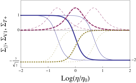
Figure 4: Evolution of $\Sigma_{{}_{\parallel}}$ (solid), $\Sigma_{{}_{\rm V}1}$ (dashed) and $\Sigma_{{}_{\rm T}+}$ (dotted) for $k_{1}\eta_{0}=k_{\perp}\eta_{0}=1$ (heavy) and $k_{1}\eta_{0}=10,k_{\perp}\eta_{0}=1$ (light) or $k_{1}\eta_{0}=1,k_{\perp}\eta_{0}=10$ (light) for a Kasner universe with $\varpi=\frac{\pi}{6}$.

Since $\Sigma_{{}_{\rm T}\times}=0$, the two polarisations decouple and their equations of evolution (63) simplify to

$$\mu_{\times,+}^{\prime\prime}+\omega^{2}_{\times,+}(k_{i},\mu)\mu_{\times,+}=0$$ (138)

with

$$\omega^{2}_{\times} = k^{2}+\frac{1}{4\eta^{2}}\left[1-2\left(\Sigma_{{}_{\rm T}+}^{2}-\Sigma_{{}_{\rm V}1}^{2}\right)\right]$$ (139)

$$\omega^{2}_{+} = k^{2}+\frac{1}{4\eta^{2}}\left[1+2\Sigma_{{}_{\rm V}1}^{2}\left(\frac{\sqrt{2}\Sigma_{{}_{\rm T}+}}{2-\Sigma_{{}_{\parallel}}}-1\right)^{2}\right]$$ (140)

where we have used that $\Sigma_{{}_{\parallel}}^{\prime}=-2\mathcal{H}\Sigma_{{}_{\rm V}1}^{2}$ and $\Sigma_{{}_{\rm T}+}^{\prime}=\sqrt{2}\mathcal{H}\Sigma_{{}_{\rm V}1}^{2}$. We emphasize that our expressions agree with those of Ref. emir (see for instance Eq. (40) of that reference).

V.2 Scalar and vector perturbations

The expressions of the scalar perturbations are therefore

$$X=\frac{\Sigma_{{}_{\rm T}+}}{2-\Sigma_{{}_{\parallel}}}\,E_{+}$$ (141)

that derives from Eq. (58) from which we deduce that Eqs. (III.4-60) reduce to

$$k^{2}\Psi = \frac{\mathcal{H}}{(2-\Sigma_{{}_{\parallel}})}\left[-\Sigma_{{}_{\rm T}+}E^{\prime}_{+}\right.$$

$$\left.+\mathcal{H}\left(\sqrt{2}\Sigma_{{}_{\rm V}1}^{2}-2\frac{\Sigma_{{}_{\rm V}1}^{2}\Sigma_{{}_{\rm T}+}}{2-\Sigma_{{}_{\parallel}}}\right)E_{+}\right]$$

and

$$\Phi_{a}=-2{\rm i}\frac{\mathcal{H}}{k}\Sigma_{{}_{\rm V}1}\left(\begin{array}[]{c}\left(\sqrt{2}-\frac{\Sigma_{{}_{\rm T}+}}{2-\Sigma_{{}_{\parallel}}}\right)E_{+}\\ \sqrt{2}E_{\times}\end{array}\right).$$ (143)

The absolute value of the coefficient in Eq. (141) evolves from $\nu_{3}^{\times}/\sqrt{2}=0$ to $\nu_{1}^{\times}/\sqrt{2}=3/\sqrt{2}$ and $\Phi_{a}$ vanishes both at early and late times.

V.3 Late time behaviour

At late times, the wave-number behaves as $k\sim k_{1}\eta/\eta_{0}$ so that $x\sim k_{1}\eta_{0}(\eta/\eta_{0})^{2}$. For the two polarisations, the growing and decaying modes entering the solution (64) behave as

$$T^{\uparrow}_{\lambda} \sim J_{0}\left[\frac{k_{1}\eta_{0}}{2}\left(\frac{\eta}{\eta_{0}}\right)^{2}\right]=J_{0}\left(\frac{x}{2}\right)$$ (144)

$$T^{\downarrow}_{\lambda} \sim N_{0}\left[\frac{k_{1}\eta_{0}}{2}\left(\frac{\eta}{\eta_{0}}\right)^{2}\right]=N_{0}\left(\frac{x}{2}\right).$$ (145)

The two modes combine to modify the phase so that the general solution is

$$E_{\lambda} \sim \frac{2A^{(\infty)}_{\lambda}}{\sqrt{\pi x}}\cos\left[\frac{x}{2}+\varphi^{(\infty)}_{\lambda}\right].$$ (146)

The behaviour of the scalar and vector perturbations are therefore easily obtained since $\beta\rightarrow\frac{\pi}{2}$, i.e.

$$\sin\beta\sim\frac{k_{\perp}}{k_{1}}\left(\frac{\eta}{\eta_{0}}\right)^{-\frac{3}{2}},\qquad\cos\beta\sim 1,$$ (147)

so that $\Sigma_{\parallel}\sim-2$ while $\Sigma_{{}_{\rm V}1}\sim 3\sin\beta$ and $\Sigma_{{}_{\rm T}+}\sim-3\sin^{2}\beta/\sqrt{2}$. It follows that

$$X \sim \frac{-3}{4\sqrt{2}}\left(\frac{k_{\perp}}{k_{1}}\right)^{2}\left(\frac{\eta}{\eta_{0}}\right)^{-3}E_{+}$$ (148)

and

$$\Phi_{a} \sim \frac{-3{\rm i}\sqrt{2}}{k_{1}\eta_{0}}\left(\frac{k_{\perp}}{k_{1}}\right)\left(\frac{\eta}{\eta_{0}}\right)^{-7/2}\left(\begin{array}[]{c}E_{+}\\ E_{\times}\end{array}\right).$$ (151)

These expressions can then be inserted in Eq. (IV.3) that is valid for $\varpi=\frac{\pi}{6}$ to conclude that at late time, the polarisations contribute in the same way to $\Xi^{(2)}$ as

$$\Xi^{(2)}_{\lambda} \to \frac{8x^{3}}{3\pi}\,,$$ (152)

which is equivalent to our prior result (116). The result for the $\times$ polarisation matches the results of Ref. emir up to normalisation factors of the transfer functions, but it appears to be different from the conclusions on the $+$ polarisation. Asymptotically, the Fourier mode is aligned with the preferred direction of the spacetime, and it turns out to be difficult to compare our result with Ref. emir given that most expressions of their formalism are singular for a mode along that special direction. We are confident that our result is correct in that limit since from Eq. (116) we find that $\bar{C}^{2}\Xi^{(2)}_{\lambda}$, which is the perturbation of the square of the Weyl, when expressed in terms of the transfer function takes the form

$$\bar{C}^{2}\Xi^{(2)}_{\lambda}\to\frac{8}{S^{4}}\left[k^{2}\left({\frac{\partial T^{\uparrow}_{\lambda}}{\partial\eta}}\right)^{2}+k^{4}{T^{\uparrow}_{\lambda}}^{2}\right].$$ (153)

This is formally the same expression as for a pure Minkowski space-time [see (Eq. 180)], which is expected when one takes the small scale limit.

V.4 Early time behaviour

At early times, the wave-number behaves as $k\sim k_{\perp}(\eta/\eta_{0})^{-\frac{1}{2}}$ so that $x\sim k_{\perp}\eta_{0}(\eta/\eta_{0})^{\frac{1}{2}}$, which goes to zero. As in § IV.5, we cannot neglect the decaying mode. We can use the expression of $\Xi^{(2)}$ obtained in § IV.5 since it is well-behaved when $q_{3}\rightarrow\frac{1}{3}$.

If we first consider the growing mode [i.e. $a_{\lambda}\neq 0$ and $b_{\lambda}=0$ in Eq. (64)] then we deduce that

$$T_{+}^{\uparrow} \sim J_{0}\left[2k_{\perp}\eta_{0}\left(\frac{\eta}{\eta_{0}}\right)^{\frac{1}{2}}\right]=J_{0}(2x)$$ (154)

$$T_{\times}^{\uparrow} \sim J_{3}\left[2k_{\perp}\eta_{0}\left(\frac{\eta}{\eta_{0}}\right)^{\frac{1}{2}}\right]=J_{3}(2x),$$ (155)

from which it follows that

$${\frac{\partial T^{\uparrow}_{\times}}{\partial\ln\eta}}\simeq\frac{3}{2}T^{\uparrow}_{\times}\qquad{\frac{\partial T^{\uparrow}_{+}}{\partial\ln\eta}}\simeq-x^{2}T^{\uparrow}_{+}.$$ (156)

Asymptotically, we have from Eq. (196) that

$$T_{+}^{\uparrow}\sim 1-x^{2},\qquad T_{\times}^{\uparrow}\sim\frac{x^{3}}{6}\,.$$ (157)

Since

$$\cos\beta\sim\frac{k_{1}}{k_{\perp}}\left(\frac{\eta}{\eta_{0}}\right)^{\frac{3}{2}},\qquad\sin\beta\sim 1,$$ (158)

$\Sigma_{\parallel}\sim 1$ while $\Sigma_{{}_{\rm V}1}\sim 3\cos\beta$ and $\Sigma_{{}_{\rm T}+}\sim-3/\sqrt{2}$ and it follows that $T_{X,\times}=T_{\Phi_{a},\times}=0$ and

$$T_{X,+}\sim\frac{-3T_{+}}{\sqrt{2}},\quad T_{\Phi_{a},+}\sim\frac{-3{\rm i}\sqrt{2}}{k_{\perp}\eta_{0}}\frac{k_{1}}{k_{\perp}}\left(\frac{\eta}{\eta_{0}}\right)\left(\begin{array}[]{c}\frac{5}{2}T_{+}\\ T_{\times}\end{array}\right).$$ (159)

With these expressions, we conclude that at leading order, the contributions of the two polarisations to $\Xi^{(2)}$ are

$$\Xi^{(2)}_{+} \to \frac{27}{2},\qquad\Xi^{(2)}_{\times}\to\frac{x^{6}}{36},$$ (160)

which both remain bounded.

On the other hand, if we consider the decaying mode [i.e. $a_{\lambda}=0$ and $b_{\lambda}\not=0$ in Eq. (64)], i.e. the most diverging mode when $x\rightarrow 0$, then

$$T_{+}^{\downarrow} \sim N_{0}\left[2k_{\perp}\eta_{0}\left(\frac{\eta}{\eta_{0}}\right)^{\frac{1}{2}}\right]=N_{0}(2x)$$ (161)

$$T_{\times}^{\downarrow} \sim N_{3}\left[2k_{\perp}\eta_{0}\left(\frac{\eta}{\eta_{0}}\right)^{\frac{1}{2}}\right]=N_{3}(2x),$$ (162)

the asymptotic behaviours of which are

$$T_{+}^{\downarrow}\sim\frac{2}{\pi}\ln\left(x\right),\qquad T_{\times}^{\downarrow}\sim-\frac{2}{\pi}x^{-3}.$$ (163)

It allows to conclude that the contributions of the two polarisations to $\Xi^{(2)}$ are

$$\Xi^{(2)}_{+}\to\frac{90}{\pi^{2}x^{4}}\,,\qquad\Xi^{(2)}_{\times}\to\frac{20}{\pi^{2}x^{6}}\,.$$ (164)

As expected both terms diverge when $\eta\rightarrow 0$.

V.5 Interpolation between the two regimes

The transition between the two asympotic regimes is illustrated on Fig. 4 for the components of the shear. While the transition is quite sharp, it is shifted depending on the value of $k_{\perp}/k_{1}$.

Then, we can integrate numerically Eq. (138) for different modes. This exact numerical solution is compared in Fig. 5 to the two asymptotic forms, which demonstrates that the transition is sharp even for the evolution of the modes. In Fig. 6, the full numerical solution of $\Xi^{(2)}_{\lambda}({\bf k},\eta)$ is compared to the two asymptotic behaviours described in §V.3 and §V.4 . This shows explicitely the validity of the asymptotic expansions.

Figure 5: Evolution of a mode with $k_{1}\eta_{0}=k_{3}\eta_{0}=10$ and $k_{2}=0$ in a Kasner universe with $\varpi=\frac{\pi}{6}$: $T_{\times}^{\uparrow}$ (left), $T_{+}^{\uparrow}$ (middle) and $T_{\Psi}^{\uparrow}$ (right) compared to their asymptotic late time (dashed) and early time (dotted) asymptotic forms. The agreement at early times is very good so that the continuous and dotted curves are hardly distinguishable.

Figure 6: Evolution of $\Xi^{(2)}_{\lambda}({\bf k},\eta)$ for a mode with $k_{1}\eta_{0}=k_{3}\eta_{0}=10$ and $k_{2}=0$ in a Kasner universe with $\varpi=\frac{\pi}{6}$ for the polarisation $\times$ (left) and $+$ (right) as well as their late time (dashed) and early time (dotted) asymptotic forms.

VI Conclusion

We have performed the stability study of a generic Kasner spacetime with respect to linear perturbations using the formalism developed in Refs. ppu1 ; ppu2 . Since Kasner spacetimes are solutions of the vacuum Einstein equations, one expects only two degrees of freedom to propagate, which we explicitely demonstrate. They can be identified with the two polarisations of gravity waves. The extra scalar and vector components of the metric are then obtained algebraically from constraint equations. Contrary to a Minkowski or de Sitter spacetime, they do not strictly vanish because the spatial sections are not isotropic anymore.

We have shown that for any Fourier mode, the behaviour of the gravity waves interpolates between two asymptotic regimes, at early and late times, in which the mode can be considered almost aligned with a principal axis of the spatial metric. Interestingly, in this limit the gravity wave equation can be integrated analytically. This allows to set a lower bound on the square of the Weyl tensor generated by the perturbations and compare it to the one of the background. We have concluded that at late time the Kasner spacetimes were unstable with respect to linear perturbations but in the particular case of $\varpi=\frac{\pi}{2}$, which corresponds to an axisymmetric configuration, product of a two-dimensional Milne spacetime and a two-dimensional Euclidean spacetime, which actually maps to one quarter of the Minkowski spacetime. At early time, the conclusion depends on the modes included in the analysis. If one includes decaying modes, the Kasner spacetimes are again unstable while stability to linear perturbations is recovered only if the growing modes are excited. This latter result was already known since Ref. bkl1 and our analysis confirms the one of Ref. emir that was limited to the particular case of an axisymmetric configuration with $\varpi=\frac{\pi}{6}$. This result is also compatible with the amplification of gravity waves during the shear dominated era of an anisotropic inflationary phase described by a Bianchi I spacetime ppu2 ; emir0 . This is amplification of a remnant of the instability described in this article for a finite Kasner era.

This result has some importance concerning the dynamics of the universe close to the singularity. On the one hand, the succession of Kasner era in the BKL formalism and the rotation of the Kasner axes from one era to the other was studied by assuming homogeneous behaviour, i.e. assuming the inhomogeneity scale was larger than the mean Hubble patch henk . The instability at early time (i.e. going toward the singularity) can alter the conclusions on the approach of the singularity, even though each Kasner era has a finite duration. In particular, as soon as the effect of the gravity wave is large enough, the backreaction would have to be taken into account, and it is not clear that the evolution toward the singularity follows a series of BKL oscillations. This requires further investigations that go beyond perturbation theory, see e.g. Ref. Deruelle . On the other hand, the instability at late time could also be relevant in models where the pre-inflationary era is described by an anisotropic era. The gravity waves modes generated during this era can potentially be observed emir2006 ; ppu2 ; emir if the number of e-folds during inflation is not too large and their presence can modify the onset of inflation.

Besides the speculative phenomenology of the early universe, our result sheds some light on the peculiarity of the Kasner spacetimes among the class of homogeneous vacuum solutions of Einstein equations.

Appendix A Different parameterisations of Kasner exponants

There exist several ways to parameterize, the coefficients $(p_{1},p_{2},p_{3})$ of the Kasner metric. Because of the two constraints (4), it is in fact a 1-parameter family of triplets that is completely specified by only one number. Three parameterisations have been widely used.

• Single exponant parameterisation. As we have seen in § II.1, it is sufficient to give one of the Kasner exponants to specify the two others. For instance, fixing the smallest one, $p_{1}$, gives that $p_{2}=1-p_{1}-p_{3}$ so that $p_{3}^{2}+(1-p_{1}-p_{3})^{2}+p_{1}^{2}=1$, from which we deduce that

  $$p_{2}=\frac{1}{2}\left[1-p_{1}-\sqrt{(1-p_{1})(1+3p_{1})}\right],$$ (165)

  $$p_{3}=\frac{1}{2}\left[1-p_{1}+\sqrt{(1-p_{1})(1+3p_{1})}\right].$$ (166)

  The two constraints (4) allow to deduce that the $p_{i}$ satisfy the following useful relations. First, $(\sum_{i}p_{i})^{2}=\sum_{i}p_{i}^{2}$ so that

  $$p_{1}p_{2}+p_{2}p_{3}+p_{3}p_{1}=0,$$ (167)

  also conveniently rewritten as

  $$\sum_{i}p_{i}^{-1}=0.$$ (168)

  From $(\sum_{i}p_{i})^{3}=1$, one deduces that

  $$\sum_{i}p_{i}^{3}=1+3\prod_{i}p_{i}.$$ (169)

  This tells us that

  $$p_{1}(p_{1}-1)=p_{2}p_{3}$$ (170)

  which implies in particular $p_{1}^{2}+p_{2}^{2}+p_{1}p_{2}-(p_{1}+p_{2})=0$, with similar relations obtained after permutation of the indices $1\to 2\to 3\to 1$. In terms of the coefficient $q_{i}$, it leads to the relations

  $$2q_{2,3}=-q_{1}\pm\Delta_{1}\,,\qquad\Delta_{1}\equiv\sqrt{\frac{4}{3}-3q_{1}^{2}}\,.$$ (171)

  In terms of the $Q_{i}=3/2q_{i}$ these relations take the simple form

  $$2Q_{2,3}=-Q_{1}\pm\sqrt{3(1-Q_{1}^{2})}\,.$$ (172)

  This shows that all the properties of the Kasner spacetime, but also the evolution of its perturbations when a mode is aligned with an eigendirection of the shear, are characterized by the choice of a single Kasner exponent corresponding to that particular direction.

• Angular parameterisation. As we have seen in § II.1, the constraints (4) imply that the triplet can be specified by a choice of an angle $\varpi\in\left[\frac{\pi}{6},\frac{\pi}{2}\right]$ and its expression is given by Eq. (5) and we have seen that

  $$\Delta_{I}\equiv\frac{2}{\sqrt{3}}|\cos\varpi_{I}|.$$ (173)

• BKL parameterisation. Refs. bkl1 ; bkl2 ; bkl3 use the parameterisation

  $$\hskip 19.91684ptp_{1}=-\frac{u}{\sigma(u)},\quad p_{2}=\frac{1+u}{\sigma(u)},\quad p_{3}=\frac{u(1+u)}{\sigma(u)},$$ (174)

  with $\sigma(u)=1+u+u^{2}$. It can be obtained kasnergen by solving the two constraints (1) once having set

  $$u=\frac{p_{3}}{p_{2}}$$ (175)

  and the condition $p_{1}\leq p_{2}\leq p_{3}$ imposes that $u\in[1,+\infty[$, with $u=1$ corresponding to $\varpi=\frac{\pi}{6}$ and $u\rightarrow+\infty$ to $\varpi=\frac{\pi}{2}$.

Appendix B Axially symmetric case with $\varpi=\frac{\pi}{2}$

The particular case $\varpi=\frac{\pi}{2}$ requires special attention. It corresponds to a spacetime with metric

$${\rm d}s^{2}=-dt^{2}+t^{2}{\rm d}z^{2}+{\rm d}x^{2}+{\rm d}y^{2},$$ (176)

which appears to be the product of a two-dimensional Milne space with a two-dimensional Euclidean space. It is the Taub representation taub of the Minkowski metric. With the change of coordinates defined by

$$(t,x,y,z)\rightarrow(T=t\cosh z,X=x,Y=y,Z=t\sinh z),$$ (177)

this metric is rewritten as

$${\rm d}s^{2}=-dT^{2}+{\rm d}Z^{2}+{\rm d}X^{2}+{\rm d}Y^{2},$$ (178)

i.e. has a Minkowski metric but only covers the patch $T^{2}-Z^{2}>0$, the upper cone ($T>0$) corresponding to an expanding universe while the lower one ($T<0$) describes a contracting spacetime. This explains why $C^{2}=0$ [Eq. (25)].

The choice of the time slicing plays an important role when studying the perturbations. In Minkowskian coordinates the spacetime is explicitely homogeneous and isotropic so that the tensor modes decouple from the other types of perturbations and evolve according to

$$\left(\partial_{T}^{2}-\Delta_{\{X,Y,Z\}}\right)h_{ij}=0.$$ (179)

Their amplitude is thus constant and the perturbation of the square of the Weyl tensor $\delta C^{2}$ remains constant. Under its Kasner form, this no more obvious and one needs to check the consistency with the result in Minkowskian coordinates

$$\delta^{(2)}C^{2}_{\lambda}=8\left[k^{2}\left({\frac{\partial T^{\uparrow}_{\lambda}}{\partial\eta}}\right)^{2}+k^{4}{T^{\uparrow}_{\lambda}}^{2}\right]$$ (180)

where the two modes have constant amplitude (so that the distinction between growing and decaying is no more relevant).

B.1 Description of the perturbation from a Kasner point of view

B.1.1 Gravity waves equation

We follow the general formalism of this article to study the perturbation in the particular case

$$q_{1}=q_{2}=-\frac{1}{3},\qquad q_{3}=\frac{2}{3}$$ (181)

so that

$$\Delta_{1}=\Delta_{2}=1,\qquad\Delta_{3}=0.$$ (182)

It implies that

$$k^{2}=k_{3}^{2}\left(\frac{\eta}{\eta_{0}}\right)^{-2}+k_{\perp}^{2}\left(\frac{\eta}{\eta_{0}}\right).$$ (183)

Obviously, this case can be deduced from the case $\varpi=\frac{\pi}{6}$ by $q_{i}\rightarrow-q_{i}$ so that the Euler angles are again

$$\tan\gamma=\frac{k_{1}}{k_{2}},\qquad\alpha=0.$$ (184)

It follows that the expressions for the shear components are also given by Eqs. (135-137) but with all signs changed, ie. $\Sigma_{{}_{\parallel}}\rightarrow-\Sigma_{{}_{\parallel}}$ etc. The evolution of the gravity waves is dictated by Eq. (138) with

$$\Sigma_{{}_{\parallel}}=-\sin^{2}\beta+2\cos^{2}\beta,$$ (185)

$$\Sigma_{{}_{\rm V}1}=-3\sin\beta\cos\beta,\qquad\Sigma_{{}_{\rm V}2}=0$$ (186)

and

$$\Sigma_{{}_{\rm T}+}=\frac{3}{\sqrt{2}}\sin^{2}\beta,\qquad\Sigma_{{}_{\rm T}\times}=0.$$ (187)

The only difference concerns the Euler angle $\beta$ which is now given by

$$\cos\beta=\frac{k_{3}}{k}\left(\frac{\eta}{\eta_{0}}\right)^{-1},\quad\sin\beta=\frac{k_{\perp}}{k}\left(\frac{\eta}{\eta_{0}}\right)^{\frac{1}{2}}.$$ (188)

B.1.2 Late time behaviour of the perturbations

In the limit $\eta\rightarrow+\infty$, $k\sim k_{\perp}(\eta/\eta_{0})^{\frac{1}{2}}$ so that $x\sim k_{\perp}\eta_{0}(\eta/\eta_{0})^{\frac{3}{2}}$. This implies that

$$\cos\beta\sim\frac{k_{3}}{k_{\perp}}\left(\frac{\eta}{\eta_{0}}\right)^{-\frac{3}{2}},\quad\sin\beta\sim 1$$ (189)

$\Sigma_{{}_{\parallel}}\sim-1$, $\Sigma_{{}_{\rm V}1}\sim-3\cos\beta$ and $\Sigma_{{}_{\rm T}+}\sim 3/\sqrt{2}$ so that we conclude

$$X\sim\frac{E_{+}}{\sqrt{2}},\quad\Phi_{a}\sim\frac{3{\rm i}\sqrt{2}}{k_{\perp}\eta_{0}}\frac{k_{3}}{k_{\perp}}\left(\frac{\eta}{\eta_{0}}\right)^{-3}\left(\begin{array}[]{c}\frac{1}{2}E_{+}\\ E_{\times}\end{array}\right).$$ (190)

The solution of the gravity wave equation is then explicitely given by

$$E_{\lambda}\sim\sqrt{\frac{3}{\pi x}}A_{\lambda}^{(\infty)}\cos\left[\frac{2}{3}x+\varphi^{(\infty)}_{\lambda}\right],$$ (191)

for the two polarisations, and where the growing and decaying modes are combined together, leading to a redefinition of the phase.

Since $\bar{C}^{2}=0$, we cannot use the variable $\Xi$ anymore and thus work directly with $\delta^{(2)}C^{2}$. In the limit $\eta\to\infty$, we obtain

$$\delta^{(2)}C^{2}_{\lambda}({\bf k},\eta) \to \frac{8x^{2}}{S^{4}\eta^{4}}\left[\left({\frac{\partial T^{\uparrow}_{\lambda}}{\partial\ln\eta}}\right)^{2}+x^{2}{T^{\uparrow}_{\lambda}}^{2}\right]$$ (192)

$$\to \frac{24x^{3}}{\pi\eta^{4}S^{4}}\propto\eta^{-\frac{3}{2}}.$$

It follows that $\delta^{(2)}C^{2}_{\lambda}$ decays at late time so that the spacetime is stable against the perturbations. Note that this is the same behaviour as for the case $\varpi\not=\frac{\pi}{2}$, but the main difference arises from the fact that $\bar{C}^{2}=0$ since in the general case $\delta^{(2)}C^{2}$ decreases with time but slower than $\bar{C}^{2}$ so that the effect of the perturbations dominate over the background quantity at late time. The stability of the Taub metric (176) was studied in Ref. taubstab with the same conclusions as our analysis.

Appendix C Bessel functions

The differential equation

$$u^{\prime\prime}+\left[\left(\beta\gamma x^{\gamma-1}\right)^{2}+\left(\frac{1}{4}-\nu^{2}\gamma^{2}\right)\frac{1}{x^{2}}\right]u=0$$ (193)

has the general solution

$$u(x)=\sqrt{x}Z_{\nu}\left[\beta x^{\gamma}\right],$$ (194)

where $Z_{\nu}$ is a linear combination of a Bessel function of the first kind ($J_{\nu}$) and of the second kind ($N_{\nu}$ or Newmann function).

We have that in $x\sim\infty$,

$$J_{\nu}(x)\sim\sqrt{\frac{2}{\pi x}}\cos\left[x-\nu\frac{\pi}{2}-\frac{\pi}{4}\right]$$ (195)

while in $x\sim 0$,

$$J_{\nu}(x)\sim\frac{1}{\Gamma(1+\nu)}\left(\frac{x}{2}\right)^{\nu}.$$ (196)

We have that in $x\sim\infty$,

$$N_{\nu}(x)\sim\sqrt{\frac{2}{\pi x}}\sin\left[x-\nu\frac{\pi}{2}-\frac{\pi}{4}\right]$$ (197)

while in $x\sim 0$,

$$N_{0}(x) \sim \frac{2}{\pi}\left[\ln\left(\frac{x}{2}\right)+\gamma_{E}\right]$$ (198)

$$N_{\nu}(x) \sim -\frac{\Gamma(\nu)}{\pi}\left(\frac{2}{x}\right)^{\nu}.$$ (199)

References

- (1) T. S. Pereira, C. Pitrou and J. P. Uzan, “Theory of cosmological perturbations in an anisotropic universe,” JCAP 0709, 006 (2007) [arXiv:0707.0736 [astro-ph]].
- (2) C. Pitrou, T. S. Pereira and J. P. Uzan, “Predictions from an anisotropic inflationary era,” JCAP 0804, 004 (2008) [arXiv:0801.3596 [astro-ph]].
- (3) A. E. Gumrukcuoglu, C. R. Contaldi and M. Peloso, “Inflationary perturbations in anisotropic backgrounds and their imprint on the CMB,” JCAP 0711, 005 (2007) [arXiv:0707.4179 [astro-ph]].
- (4) A. E. Gumrukcuoglu, L. Kofman and M. Peloso, “Gravity waves signatures from anisotropic pre-inflation,” Phys. Rev. D 78, 103525 (2008) [arXiv:0807.1335 [astro-ph]].
- (5) E. Kasner, “Geometrical theorems on Einstein’s cosmological equations”, Am. J. Math. 43, 217 (1921).
- (6) E.M. Lifshitz and I.M. Khalatnikov, “Investigations in relativistic cosmology”, Adv. Phys. 12, 185 (1963).
- (7) V.A. Belinskii, I.M. Khalatnikov, and E.M. Lifshttz, “Oscillatory approach to a singular point in the relativistic cosmology” Adv. Phys. 19 525 (1970).
- (8) V. A. Belinskii, I.M. Khalatnikov, and E.M. Lifshitz, “A general solution of the Einstein equations with a time singularity”, Adv. Phys. 31 639 (1982).
- (9) C.W. Misner, “Mixmaster universe”, Phys. Rev. Lett. 22 1071 (1969).
- (10) T. Damour, M. Henneaux and H. Nicolai, “Cosmological billiards”, Class. Quant. Grav. 20, R145 (2003) [arXiv:hep-th/0212256].
- (11) B.L. Hu and T. Regge, “Numerical examples from perturbation analysis of the Mixmaster universe”, Phys. Rev. Lett. 29, 1616 (1972).
- (12) B.L. Hu, “Perturbations the Mixmaster universe”, Phys. Rev. D 12, 1551 (1975).
- (13) P.J. Adams, et al., “Inhomogeneous cosmology: gravitational radiation in Bianchi backgrounds”, Astrophys. J. 253, 1 (1982).
- (14) D. Christodoulou and S. Klainerman, The global nonlinear stability of the Minkowski space’, (Princeton University Press, 1993).
- (15) A.S. Eddington, Month. Not. R. Astron. Soc. 90, 668 (1930).
- (16) E.R. Harrison, “Normal modes of vibrations of the Universe” Rev. Mod. Phys. 39, 862 (1967).
- (17) G.W. Gibbons, “The entropy and stability of the universe”, Nucl. Phys. B 292, 784 (1987); G.W. Gibbons, “Sobolevs inequality, Jensens theorem and the mass and entropy of the Universe”, Nucl. Phys. B 310, 636 (1988).
- (18) J.D. Barrow et al., “On the stability of the einstein static universe”, Class. Quant. Grav. 20, L155 (2003), [arXiv:astro-ph/0302094].
- (19) H. Stephani et al., Exact solutions to Einstein’s field equations, (Cambridge University Press, 2003).
- (20) P. Peter and J.-P. Uzan, Primordial cosmology (Oxford Univ. Press, England, 2009).
- (21) D. Bini, C. Cherubini, and R.T. Jantzen, “The Lifshitz-Khalatnikov Kasner index parametrization and the Weyl tensor”, [arXiv:0710.4902].
- (22) L. Andersson et al., “Asymptotic silence of generic cosmological singularities”, Phys. Rev. Lett. 94, 051101 (2005), [arXiv:gr-qc/0402051].
- (23) N. Deruelle and D. Langlois, “Long wavelength iteration of Einstein’s equations near a space-time singularity”, Phys. Rev. D 52, 2007 (1995), [arXiv:gr-qc/9411040].
- (24) A. E. Gumrukcuoglu, C. R. Contaldi and M. Peloso, “CMB anomalies from relic anisotropy”, [arXiv:astro-ph/0608405].
- (25) A.H. Taub, “Empty space-times admitting a three parameter group of motions”, Ann. Math. 53, 472 (1951).
- (26) S. Bonanos, “On the stability of the Taub universe”, Comm. Math. Phys. 22, 190 (1971); S. Bonanos, “Stability of homogeneous universes” Comm. Math. Phys. 26, 259 (1972).