Reconstructing phase dynamics of oscillator networks

Abstract

We generalize our recent approach to reconstruction of phase dynamics of coupled oscillators from data [B. Kralemann et al., Phys. Rev. E, 77, 066205 (2008)] to cover the case of small networks of coupled periodic units. Starting from the multivariate time series, we first reconstruct genuine phases and then obtain the coupling functions in terms of these phases. The partial norms of these coupling functions quantify directed coupling between oscillators. We illustrate the method by different network motifs for three coupled oscillators and for random networks of five and nine units. We also discuss nonlinear effects in coupling.

Many natural and technological systems can be described as networks of coupled oscillators. A typical problem in their analysis is to find dynamical features, e.g., synchronization, transition to chaos, etc., in dependence on the properties of oscillators and of the coupling. Here we address the inverse problem: how to find the properties of the coupling from the observed dynamics of the oscillators. This may be relevant for many experimental situations, where the equations of underlying dynamics are not known. We present here a method which is based on invariant reconstruction of phase dynamics equations from multivariate observations (at least one scalar oscillating observable of each oscillator must be available) and includes several algorithmic steps which are rather easy to implement numerically. We illustrate the method by numerical examples of small networks of van der Pol oscillators.

I Introduction

Dynamics of coupled self-sustained oscillators attracts vast interest of researchers, both due to a variety of nontrivial effects and to numerous applications in physics, chemistry, and life sciences. In modeling, one usually focuses on the relations of the dynamical features, such as synchronization patterns, to the coupling structure of the underlying network. In experimental data analysis, an inverse problem typically arises, where one wants to reveal the interactions from the observed dynamics. A simple consideration demonstrates that this task is really challenging and highly nontrivial: indeed, computation of correlations and or synchronization index between the oscillators does not solve the problem, because the interactions are generally non-reciprocal while both the correlation and the synchronization index are symmetric measures.

There are exist two approaches for the determination of directional coupling. The first one exploits various information-theoretical techniques and quantifies an interaction with the help of such asymmetric measures as transfer entropy, Granger causality, predictability, etc. Schreiber-00 ; Frenzel-Pompe-07 ; Ishiguro_et_al-08 ; Chicharro-Andrzejak-09 ; Faes_et_al-08 . The second approach, developed in our previous publications Rosenblum-Pikovsky-01 ; Rosenblum_et_al-02 , see also Smirnov-Bezruchko-03 , is based on estimation of phases from oscillatory time series and subsequent reconstruction of phase dynamics equations and quantification of coupling by inspecting and quantifying the structure of these equations. The disadvantage of the second, dynamical, approach in comparison to the information-theoretical one is that it is restricted to the case of weakly coupled oscillatory systems. However, for this widely encountered case the dynamical approach has clear advantages: it works with phases, which are most sensitive to interaction, and yields description of connectivity which admits a simple interpretation. This consideration is supported by several comparative studies Smirnov-Andrzejak-05 ; Smirnov_et_al-07 . (Notice that there is an intermediate group of techniques which apply informatical measures to time series of phases Rosenblum_et_al-02 ; Palus-Stefanovska-03 ; Vejmelka-Palus-08 ; Bahraminasab_et_al-08 .) The dynamical approach has been tested in a physical experiment Bezruchko-Ponomarenko-Pikovsky-Rosenblum-03 and used for analysis of connectivity in a network of two or several oscillators in the context of cardio-respiratory interaction Mrowka_et_al-03 , brain activity Cimponeriu_et_al-03 ; Schnitzler-Gross-05 ; Osterhage_et_al-08 , and climate dynamics Mokhov-Smirnov-06 .

Recently, we have essentially improved the dynamical approach by suggesting a technique for invariant reconstruction of the phase dynamics equations from bivariate time series Kralemann_et_al-07 ; Kralemann_et_al-08 ; damoco . Invariance in this context means that reconstructed equations do not depend on the observables used (at least for a wide class of observables). This technique was tested on numerical examples as well as in physical experiments with coupled metronomes Kralemann_et_al-07 ; Kralemann_et_al-08 and with electro-chemical oscillators Blaha_et_al-11 . In this paper we extend the technique to cover the case of small networks of interacting oscillators. The paper is organized as follows. In Section II we discuss phase description of oscillator network. In Section III we describe the basic method; it is illustrated in Sections IV and V. We summarize and discuss our results in Section VI.

II Phase description of oscillator network

We assume that an individual oscillator is described by variables $\mathbf{x}$ which satisfy a system of ODEs $\dot{\mathbf{x}}=\mathbf{G}(\mathbf{x})$ and that this equation system possesses a stable limit cycle. The latter can be parameterized by phase $\varphi$ which grows uniformly in time, $\dot{\varphi}=\omega=\mbox{const}$, where $\omega$ is the oscillation frequency. Notably, this phase parameterization is unique (up to trivial shifts) and invariant with respect to variable transformations Kuramoto-84 ; Pikovsky-Rosenblum-Kurths-01 .

A network of $N$ oscillators can be represented as

$$\dot{\mathbf{x}}_{k}=\mathbf{G}_{k}(\mathbf{x}_{k})+\mathbf{H}_{k}(\mathbf{x}_{1},\mathbf{x}_{2},\ldots)\;,\quad k=1,\ldots,N\;,$$ (1)

where coupling functions $\mathbf{H}_{k}$ generally depend on the states of all oscillators. If variables $\mathbf{x}_{l}$ are absent in $\mathbf{H}_{k}$, we say that there is no direct coupling from $l$ to $k$. Note that generally the oscillators can be quite different, e.g., even the dimensions of state variables $\mathbf{x}_{k}$ can differ. Of course, the functions $\mathbf{G}_{k}$ can be different as well.

Assuming weakness of the coupling, one can reduce network equations Eq. (1) to phase equations

$$\dot{\varphi}_{k}=\omega_{k}+h_{k}(\varphi_{1},\varphi_{2},\ldots)\;,\quad k=1,\ldots,N\;,$$ (2)

using a perturbation technique (see Kuramoto-84 ; Pikovsky-Rosenblum-Kurths-01 for details). Then, in the first approximation, $h_{k}$ depends explicitly on phase $\varphi_{l}$ only if $\mathbf{H}_{k}$ depends explicitly on $\mathbf{x}_{l}$, i.e. if there exists a direct link $l\to k$. However, in the higher approximations, the r.h.s. of Eq. (2) may contain high-order terms which depend not only on phases of directly coupled oscillators, but on the other phases as well. Thus, generally speaking, phase oscillators Eq. (2) are all-to-all coupled. Nevertheless, as shown in Section III below, we can decompose the coupling functions $h_{k}$ into several components, and comparing the norms of these components, characterize the partial couplings between particular nodes. In fact, we attribute links only to those nodes for which the corresponding norms are sufficiently large. Reconstructed in this way, the structure of the phase network (2) correctly (although not exactly) represents the original network (1).

To specify the relation between the original network structure and that of the phase oscillators, we introduce the following terminology. If the function $\mathbf{H}_{k}$ can be written as $\mathbf{H}_{k}=\sum_{j\neq k}H_{kj}(\mathbf{x}_{k},\mathbf{x}_{j})$, we call this type of coupling pairwise. Other terms, containing a combination of several variables acting on $k$, e.g. $H_{kjl}(\mathbf{x}_{k},\mathbf{x}_{j},\mathbf{x}_{l})$, we call cross-coupling terms. If the coupling is pairwise and weak, then a perturbative phase reduction yields, in the leading order, only pairwise terms like $h_{kj}(\varphi_{k},\varphi_{j})$ in the system (2) . As discussed above, cross-coupling terms in the phase system (2) which depend on two or more driving phases, appear either due to cross-coupling terms in the original system (1) or, if the latter has pairwise couplings only, due to high-order combinational terms which appear in the perturbative reduction to phase dynamics.

We emphasize that validity of the phase equations (2) is not restricted to the case of very small coupling. Indeed, these equations are valid as long as an attracting invariant torus exists in the phase space of the full system (1). This torus can also exist for parameters of coupling when a perturbation approach is not valid anymore. In this case, Eq. (2) cannot be derived from Eq. (1) by means of a perturbation technique, but can be, however, reconstructed numerically from multivariate time series. Here, of course, the relation between networks (2) and (1) is nontrivial; in particular, some nodes may appear as connected in (2) while being disconnected in (1).

The main idea of our approach is to reconstruct the phase dynamics (2) from multivariate time series; here it is assumed that $k$th component of the series represents the output of the $k$th oscillator. Before proceeding with the description of the method, we make a remark on the range of its validity. An important dynamical regime in system (2) is that of full or partial synchrony, when the dynamics of the phases reduces to a stable torus of lower dimension (partial synchrony) or to a stable limit cycle (if all oscillators are synchronized). In case of synchrony our technique fails, because the data points do not cover the original $N$-dimensional torus and the coupling functions cannot be reconstructed. Sufficiently strong noise could cause deviation of the trajectory from the synchronization manifold and help to infer the dynamics, but discussion of this case goes beyond the scope of this paper.

III Reconstruction of phase dynamics from data

The main assumption behind our approach is that we have multivariate observations of coupled oscillators, where at least one scalar oscillating time series $y_{k}(t)=y_{k}(\mathbf{x}_{k}(t))$ is available for each oscillator. The first step is to transform this observable into a cyclic observable. Typically this is done via construction of a two-dimensional embedding $(y_{k},\bar{y}_{k})$, where $\bar{y}$ can be, e.g., the Hilbert transform of $y(t)$, see Pikovsky-Rosenblum-Kurths-01 ; Kralemann_et_al-08 for a detailed discussion. Alternatively, one can use for $\bar{y}$ the time derivative of $y$. (In all cases the data usually requires some preprocessing, e.g., filtering). If the trajectory in the plane $(y_{k},\bar{y}_{k})$ rotates around some center, one can compute a cyclic variable $\theta_{i}(t)$, e.g., by means of the arctan function. As has been in detail argued in Kralemann_et_al-08 , in this way we obtain not the genuine phase $\varphi_{k}$ of the oscillator which enters Eq. (2)), but a cyclic variable, or protophase. The latter depends on the particular embedding and on the parameterization of rotations, and is therefore not invariant. This can be seen already from the analysis of an autonomous oscillator: the described procedure generally yields a protophase $\theta(t)$ which rotates not uniformely, but obeys

$$\dot{\theta}=f(\theta)\;.$$

The transformation to the uniformly rotating genuine phase $\varphi$ reads

$$\varphi(\theta)=\omega\int_{0}^{\theta}\frac{\text{d}\theta^{\prime}}{f(\theta^{\prime})}\;,$$

where $\omega=2\pi\left[\int_{0}^{2\pi}f^{-1}(\theta^{\prime})\text{d}\theta^{\prime}\right]^{-1}$ is the frequency of oscillations. For practical reason it is convenient to determine not the function $f$, but the probability density of the protophase $\sigma(\theta)=\frac{\omega}{2\pi f(\theta)}$. Thus, the transformation from the protophase $\theta$ to the phase $\varphi$ can be written as

$$\varphi(\theta)=2\pi\int_{0}^{\theta}\text{d}\theta^{\prime}\;\sigma(\theta^{\prime})\;.$$

Hence, determination of the genuine phase from the data reduces to a problem of finding the probability distribution density of the obtained protophase $\theta$, which is a standard task in the statistical data analysis. Practically, one can use either a Fourier representation of the density $\sigma(\theta)$, as in Kralemann_et_al-08 , or a kernel function representation of $\sigma(\theta)$.

After the transformation $\theta_{k}(t)\to\varphi_{k}(t)$ is performed, we reconstruct the phase dynamics making use of the fact that the time derivatives $\dot{\varphi}_{k}$ are $2\pi$-periodic functions of the phases, in accordance with Eq. (2). These functions can be obtained from the observed multivariate time series of phases $\Phi_{k}(t)$ with the help of a spectral representation technique Kralemann_et_al-08 or by means of a kernel function estimation. Here we present the formulae for the spectral technique (see Sec. IV-A in Kralemann_et_al-08 for details), generalized for the case of more than two oscillators:

$$F^{(k)}(\varphi_{1},\varphi_{2},\ldots) =\frac{F_{u}^{(k)}(\varphi_{1},\varphi_{2},\ldots)}{F_{d}^{(k)}(\varphi_{1},\varphi_{2},\ldots)}\;,$$ (3)

$$F_{u,d} =\sum_{l_{1},l_{2},\ldots}f^{(u,d)}_{l_{1},l_{2},\ldots}\exp(il_{1}\varphi_{1}+il_{2}\varphi_{2}+\ldots)\;,$$

$$f^{(u)}_{l_{1},l_{2},\ldots} =\frac{1}{T}\int_{0}^{\Phi_{k}(T)}\text{d}\Phi_{k}\,\exp(il_{1}\Phi_{1}+il_{2}\Phi_{2}+\ldots)\;,$$

$$f^{(d)}_{l_{1},l_{2},\ldots} =\frac{1}{T}\int_{0}^{T}\text{d}t\,\exp(il_{1}\Phi_{1}+il_{2}\Phi_{2}+\ldots)\;.$$

As a result, we obtain the system of the phase dynamics equations in the form

$$\frac{d\varphi_{k}}{dt}=F^{(k)}(\varphi_{1},\varphi_{2},\ldots)=\sum_{l_{1},l_{2},\ldots}\mathcal{F}^{(k)}_{l_{1},l_{2},\ldots}\exp(il_{1}\varphi_{1}+il_{2}\varphi_{2}+\ldots)\;.$$ (4)

The coupling functions $F^{(k)}$ describe all types of interactions: pairwise, triple-wise, quadruple-wise, and so on. To characterize them separately, we calculate the norms of different coupling terms (the partial norms), as follows. The term $\mathcal{F}^{k}_{0,0,\ldots}$ is a constant (phase-independent) one, it corresponds to the natural frequency of oscillations. The pairwise action of oscillator $j$ on oscillator $k$ is determined by those components of $F^{(k)}$ which depend on phases $\varphi_{k}$ and $\varphi_{j}$ only. We quantify this action by the partial norm ${\cal N}^{(2)}_{k|j}$; note that here the upper index corresponds to the order of interaction (pairwise here). The partial norm can be computed as

$$\left[{\cal N}^{(2)}_{k|j}\right]^{2}=\sum_{l_{k};l_{j}\neq 0}\left|\mathcal{F}^{(k)}_{0,\ldots,0,l_{k},0,\ldots,0,l_{j},0,\ldots)}\right|^{2}\;.$$ (5)

Correspondingly, the joint action of oscillators $j,m$ on oscillator $k$ is determined by the cross-coupling terms containing three phases $\varphi_{k},\varphi_{j},\varphi_{m}$. This action is quantified by the following partial norm:

$$\left[{\cal N}^{(3)}_{k|jm}\right]^{2}=\sum_{l_{k};l_{j}\neq 0;l_{m}\neq 0}\left|\mathcal{F}^{(k)}_{0,\ldots,0,l_{k},0,\ldots,0,l_{j},0,\ldots,0,l_{m},0,\ldots)}\right|^{2}\;.$$ (6)

Similarly we can compute the partial norm ${\cal N}^{(4)}_{k|jmn}$, and so on.

Now we discuss the terms $\mathcal{F}^{(k)}_{0,\ldots,0,l_{k},0,\ldots,0}$ which depend only on one phase $\varphi_{k}$ and therefore cannot be attributed to any interaction. In Ref. Kralemann_et_al-08 we used an additional transformation $\varphi\to\varphi^{\prime}$ which eliminated these terms, using some additional assumptions on the structure of coupling. In examples presented below we checked that the difference between the formulations in terms of $\varphi$ and $\varphi^{\prime}$ is rather small. Therefore we use the technique described above and neglect the small terms $\mathcal{F}^{(k)}_{0,\ldots,0,l_{k},0,\ldots,0}$.

IV Case study: Three coupled van der Pol oscillators

In this section we test the presented technique on a system of three coupled van der Pol oscillators:

$$\ddot{x}_{1}-\mu(1-x_{1}^{2})\dot{x}_{1}+\omega_{1}^{2}x_{1} =\Delta\left[\sigma_{12}(\dot{x}_{2}+x_{2})+\sigma_{13}(\dot{x}_{3}+x_{3})\right]$$ (7)

$$+\sigma_{11}\eta x_{2}x_{3}\;,$$

$$\ddot{x}_{2}-\mu(1-x_{2}^{2})\dot{x}_{2}+\omega_{2}^{2}x_{2} =\Delta\left[\sigma_{21}(\dot{x}_{1}+x_{1})+\sigma_{23}(\dot{x}_{3}+x_{3})\right]$$

$$+\sigma_{22}\eta x_{1}x_{3}\;,$$

$$\ddot{x}_{3}-\mu(1-x_{3}^{2})\dot{x}_{3}+\omega_{3}^{2}x_{3} =\Delta\left[\sigma_{31}(\dot{x}_{1}+x_{1})+\sigma_{32}(\dot{x}_{2}+x_{2})\right]$$

$$+\sigma_{33}\eta x_{1}x_{2}\;.$$

Here the matrix $\sigma_{kl}$, with entries zero and one, determines the coupling structure (topology) of the network: for non-diagonal terms, $\sigma_{kl}=1$, if there is forcing from oscillator $l$ to oscillator $k$, and $\sigma_{kl}=0$, otherwise. Diagonal terms $\sigma_{kk}$ determine the presence or absence of cross-coupling. Parameters $\Delta$ and $\eta$ describe the intensity of pairwise and cross-coupling, respectively. In all examples of this section we use the values of parameters $\mu=0.5,\;\omega_{1}=1,\;\omega_{2}=1.3247,\;\omega_{3}=1.75483$. Equations (7) have been solved by the Runge-Kutta method, and the time series of $x_{k},\dot{x}_{k}$ were used to calculate the protophases as $\theta_{k}=-\text{arctan}(\dot{x}_{k},x_{k})$. The data sets consisted of $10^{6}$ or $10^{7}$ points sampled with $0.01$ time step. The analyzed coupling configurations are schematically given in Fig. 1. Note that we chose the oscillator frequencies and parameters of coupling so that network remains asynchronous.

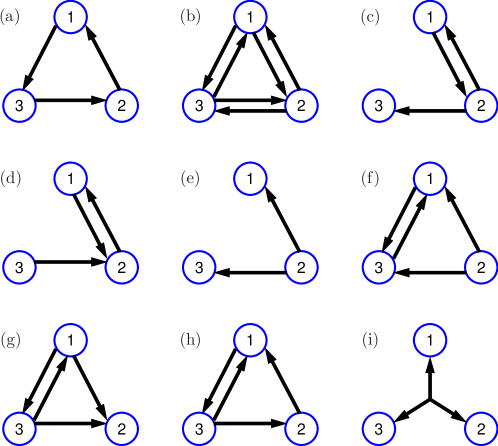
Figure 1: Different configurations in a network of 3 oscillators. (a)-(h): pairwise interaction. Panel (i) illustrates cross-coupling: an arrow from the center to, say, first oscillator reflects the term $\sim x_{2}x_{3}$ with $\sigma_{11}=1$ in Eq. (7), etc.

In the first set of tests we considered only pairwise coupling in Eqs. (7), i.e. we took $\sigma_{kk}=0$. The results for $\Delta=0.05$ and $\Delta=0.15$ are presented in Figs. 2,3, respectively. Here in the left column we schematically show the reconstructed coupling configuration. The corresponding partial norms are coded by the width of arrows which link the nodes. Only norms which are larger than $10\%$ of the maximal norm are shown here. The numerical values of all reconstructed norms can be seen in the tables in the right column. Here we show the coupling norms for the pairwise coupling (5) as non-diagonal terms, and the triple-phase coupling according to (6) as diagonal ones. The coupling terms, which are present in the original system (7) (i.e. those with $\sigma_{kl}=1$) are shown in boxes. We see that in all cases these terms are definitely larger than other entries of the reconstructed coupling matrix, i.e. the reconstruction works pretty well in all cases. Comparing the results for smaller and larger coupling (Fig. 2 and 3, respectively), we see that larger coupling strength leads to appearance of cross-coupling terms for phases that are not present in the original system (7).

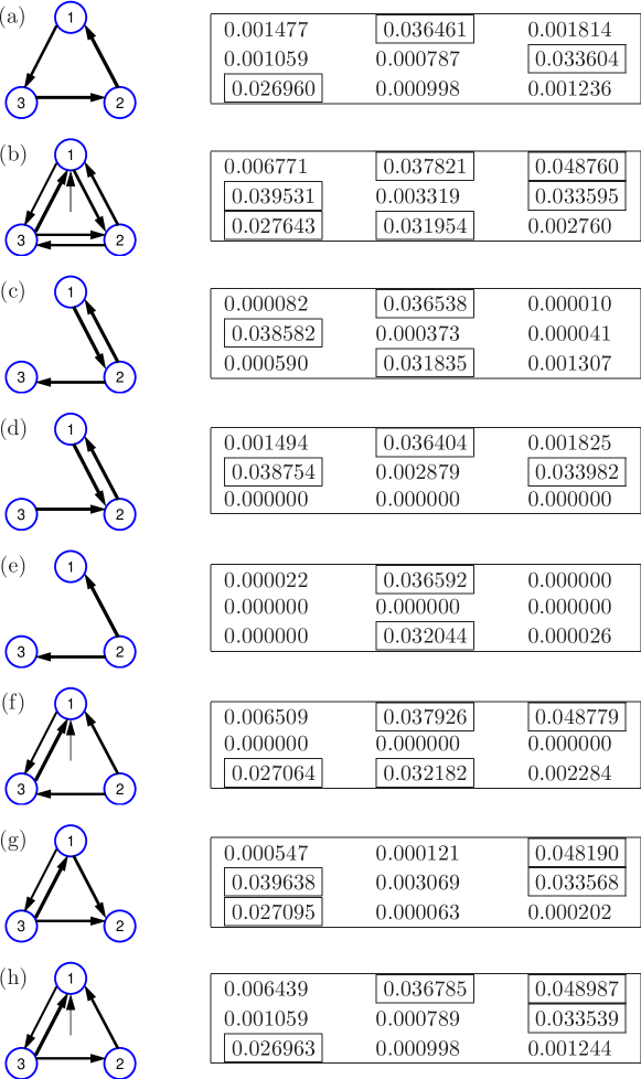
Figure 2: Reconsructed network configurations, to be compared with the true configurations, shown in Fig. 1(a-h). Each panel shows the partial norms of reconstructed coupling functions as a table; the numbers in boxes correspond to truly existing links, so ideally the numbers without the boxes should be zero. Pictures present the largest norms only (see text); the values of the norms are coded by width of linking arrows. The arrows from the center to the first oscillator (see panels (b), (f), and (h)) reflect the joint action from oscillators 2 and 3 which cannot be decomposed into pairwise actions $2\to 1$ and $3\to 1$. Coupling strength $\Delta=0.05$ and $\eta=0$.

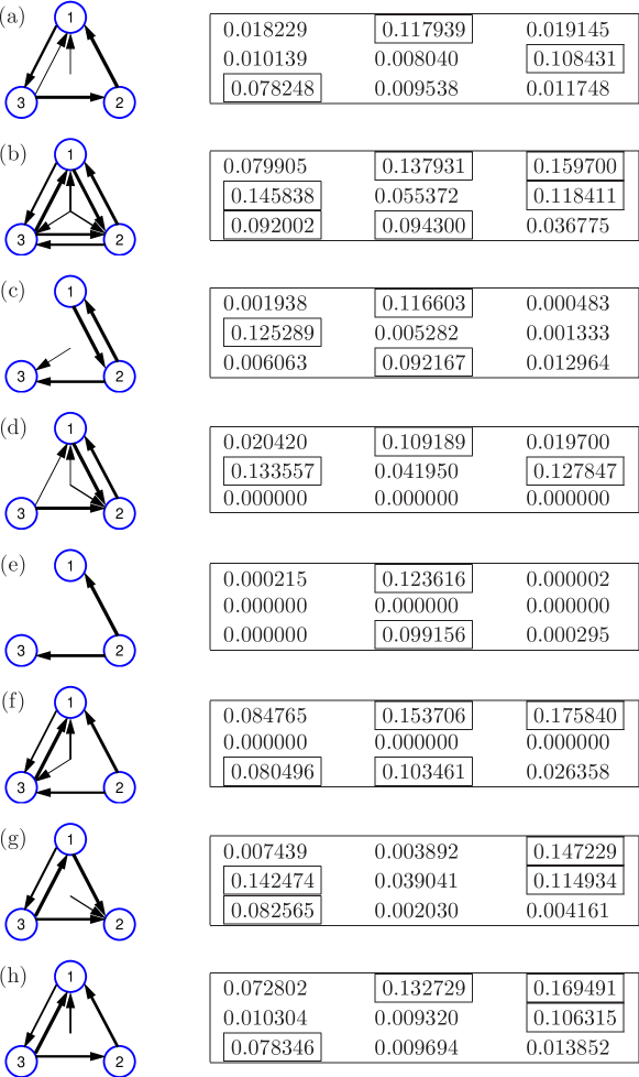
Figure 3: Same as Fig. 2, but for $\Delta=0.15$.

In the second set of tests we included the cross-couplings by setting $\sigma_{kk}=1$ and $\eta=0.1$. So, each configuration shown in Fig. 1(a-h) was complimented by the links according to Fig. 1(i). The results are presented in Fig. 4. We see that basically the coupling structure is correctly reproduced by the method, although due to a joint action of different terms some couplings, not presented in the original system (7), do not fall below $10\%$ of the largest norm.

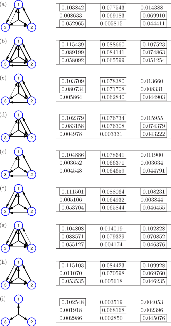
Figure 4: Same as Fig. 2, but for combination of pairwise and triple-coupling, $\Delta=0.1$, $\eta=0.1$. Panels (a-h) correspond to combination of pairwise coupling as shown in Fig. 1(a-h) with the triple-coupling as in Fig. 1(i). Panel (i) shows the results for purely triple-coupling.

Summarizing the results of this section, we conclude that the connectivity of a weakly and pairwisely coupled network can be correctly revealed. For stronger coupling, all really existing in the original network links are correctly revealed and some additional links appear. However, the latter are not necessarily spurios. Indeed, as discussed above, not very weak pairwise coupling in the original network may lead to additional connections in the network of phase oscillators and to cross-coupling terms. Our results are in full agreement with this argument.

V Case study: Networks of five and nine oscillators

In this section we report on the results for small networks of $N=5$ and $N=9$ coupled van der Pol oscillators. We simulated the systems with pairwise interaction only:

$$\ddot{x}_{k}-\mu(1-x_{k}^{2})\dot{x}_{k}+\omega_{i}^{2}x_{k}=\Delta\sum_{l\neq k}\sigma_{kl}(x_{l}\cos\alpha_{kl}+\dot{x}_{l}\sin\alpha_{kl})\;.$$ (8)

As above, $\mu=0.5$, $\Delta$ is intensity of coupling, and $\sigma_{kl}$ is the $N\times N$ connectivity matrix ($\sigma_{kl}=1$ if oscillator $l$ acts on oscillator $k$, and $\sigma_{kl}=0$ otherwise). An additional parameter $\alpha_{kl}$ describes the phase shift in the coupling, so that generally the latter can be both attracting or repelling.

We note that computational efforts and data requirements for reconstruction of a network of $N$ oscillators grow rapidly with $N$, so that full reconstruction for $N>3$, though theoretically possible, see Eqs. (3,4), becomes practically unfeasible. On the other hand, in the previous section we have verified that weak pairwise couplings can be reliably recovered. Therefore, for networks described by Eqs. (8) we reconstruct pairwise coupling functions only, for all pairs of network units.

We performed a statistical analysis of the model (8): for many randomly chosen values of frequencies $\omega_{k}$, parameters $\alpha_{kl}$, and connectivity matrices $\sigma_{kl}$ we analysed pairwise interactions in the networks. For $N=5$, the frequencies $\omega_{k}$ have been chosen uniformly distributed in $(0.5,1.5)$, and the number of incoming links for each node was 2 (i.e. $\sum_{l}\sigma_{kl}=2$), while the links have been chosen randomly (the incoming and outgoing links were chosen independently). For $N=9$, the frequencies $\omega$ were distributed uniformly in $(0.5,2.5)$, and the number of incoming links was 3. The intensity of coupling in both cases was $\Delta=0.15$, the phase shift $\alpha_{kl}$ was distributed uniformly in $[0,2\pi)$.

For each network we computed $N$ protophases according to $\theta_{k}=-\text{arctan}(\dot{x}_{k},\omega_{k}x_{k})$ and then transformed them to phases $\varphi_{k}$. Next, synchronization analysis have been performed: for all pairs we calculated the synchronization index $|\langle e^{i(\varphi_{k}-\varphi_{l})}\rangle|$. Since our technique does not work in case of synchrony, we excluded from the further consideration all networks where synchronization index was larger than $0.5$ at least for one link.

For each obtained non-synchronous network we fitted the time derivatives $\dot{\varphi}_{k}$ by $\sum_{k\neq l}F_{kl}(\varphi_{k},\varphi_{l})$, where $F_{kl}$ depend on two phases only. Next, we computed norms ${\cal N}_{kl}$ of all $F_{kl}$; these norms represent reconstructed connectivity of the network. Performing the analysis with a large ensemble of non-synchronous networks, we separated ${\cal N}_{kl}$ into two classes: first class contains those values of ${\cal N}_{kl}$ for which $\sigma_{kl}=1$, i.e. the connections between nodes $k,l$ in the network (8) really exists. Otherwise, if $\sigma_{kl}=0$, the value ${\cal N}_{kl}$ belongs to the second class. The obtained results are summarized in Fig. 5. Ideally, one would expect that all norms in the first class are much larger than those in the second one (cf. Figs. 2,3). We see that there is a clear, although not ideal, separation between connected and non-connected links, what allows us to conclude that generally our technique correctly reproduces the network structure. However, a more detailed statistical analysis is needed before a “blind” application of the method would be possible.

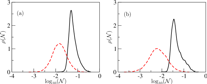
Figure 5: Probability distribution densities $\rho({\cal N})$ of the norms of reconstructed couplings: black solid line: really present connections ($\sigma_{kl}=1$), dashed red line: absent connections ($\sigma_{kl}=0$), for networks (8) of 5 (a) and 9 (b) oscillators.

VI Discussion and conclusion

In summary, we have presented a technique for reconstruction of the phase model of a network of coupled limit cycle oscillators. From the reconstructed model we infer directional couplings of the network. We have tested the technique on small networks of van der Pol oscillators with pairwise and cross-coupling. We have shown, that presence and direction of existing links can be reliably revealed. However, if the coupling is not very weak, the technique yields additional links which are absent in the original network. The differentiation between the truly existing and additional links is not perfect. Now we discuss where the additional links come from. First, some additional links may be numerical artefacts (spurious links). They may appear due to noise, closeness to sychrony, neglection of the amplitude information, etc. Second, some links, absent in the model in terms of state variables, should indeed be present in the phase model and are, therefore, not spurious. If we asume that a matrix $\sigma_{kl}$ determines the structural connectivity of the original network model (1), then the phase model (2) for this network would have an effective connectivity matrix $\Sigma_{kl}$ with a larger number of links and possibly with many cross-couplings. It is this effective connectivity that is determined in our approach, not the original one. Moreover, here one should distinguish between the structural connectivity (described by matrices $\sigma,\Sigma$) and the functional one, which is described by similarities in the dynamics (e.g. via correlations or synchronization). The functional connectivity (this term, typically used in the context of analysis of brain activity, is widely understood as a correlated time behavior) results from the dynamics, and may only loosely correspond to the structural one Tass_et_al-98 ; Shelter_et_al-06 .

Finally, we discuss the perspectives of the analysis of networks of many oscillators. As we have demonstrated, generally a pairwise analysis yields good results only if the connections are pairwise and weak. In the case of cross-coupling (see e.g., Fig. 1(i)), pairwise analysis does not help. Determination of applicability of a pairwise analysis for a given network remains an open problem. A possible solution might be reconstruction of phase dynamics for several or all triplets of oscillators and comparison of the terms, dependent on three phases, with those dependent only on two. If the triple terms are much smaller in norm than pairwise ones, than the pairwise analysis may be sufficient.

- (1) T. Schreiber, “Measuring information transfer,” Phys. Rev. Lett. 85, 461–464 (2000).
- (2) S. Frenzel and B. Pompe, “Partial mutual information for coupling analysis of multivariate time series,” Phys. Rev. Lett. 99, 204101 (Nov 2007).
- (3) K. Ishiguro, N. Otsu, M. Lungarella, and Y. Kuniyoshi, “Detecting direction of causal interactions between dynamically coupled signals,” Phys. Rev. E 77, 026216 (Feb 2008).
- (4) D. Chicharro and R. G. Andrzejak, “Reliable detection of directional couplings using rank statistics,” Phys. Rev. E 80, 026217 (Aug 2009).
- (5) L. Faes, A. Porta, and G. Nollo, “Mutual nonlinear prediction as a tool to evaluate coupling strength and directionality in bivariate time series: Comparison among different strategies based on nearest neighbors,” Phys. Rev. E 78, 026201 (Aug 2008).
- (6) M. G. Rosenblum and A. S. Pikovsky, “Detecting direction of coupling in interacting oscillators,” Phys. Rev. E 64, 045202 (2001).
- (7) M. G. Rosenblum, L. Cimponeriu, A. Bezerianos, A. Patzak, and R. Mrowka, “Identification of coupling direction: Application to cardiorespiratory interaction,” Phys. Rev. E 65, 041909 (2002).
- (8) D. A. Smirnov and B. P. Bezruchko, “Estimation of interaction strength and direction from short and noisy time series,” Phys. Rev. E 68, 046209 (Oct 2003).
- (9) D. A. Smirnov and R. G. Andrzejak, “Detection of weak directional coupling: Phase-dynamics approach versus state-space approach,” Phys. Rev. E 71, 036207 (Mar 2005).
- (10) D. Smirnov, B. Schelter, M. Winterhalder, and J. Timmer, “Revealing direction of coupling between neuronal oscillators from time series: Phase dynamics modeling versus partial directed coherence,” Chaos 17, 013111 (2007).
- (11) M. Paluŝ and A. Stefanovska, “Direction of coupling from phases of interacting oscillators: An information-theoretic approach,” Phys. Rev. E 67, 055201 (2003).
- (12) M. Vejmelka and M. Paluš, “Inferring the directionality of coupling with conditional mutual information,” Phys. Rev. E 77, 026214 (Feb 2008).
- (13) A. Bahraminasab, F. Ghasemi, A. Stefanovska, P. V. E. McClintock, and H. Kantz, “Direction of coupling from phases of interacting oscillators: A permutation information approach,” Phys. Rev. Lett. 100, 084101 (Feb 2008).
- (14) B. P. Bezruchko, V. Ponomarenko, A. S. Pikovsky, and M. G. Rosenblum, “Characterizing direction of coupling from experimental observations,” Chaos 13, 179–184 (2003).
- (15) R. Mrowka, L. Cimponeriu, A. Patzak, and M.G. Rosenblum, “Directionality of coupling of physiological subsystems - age related changes of cardiorespiratory interaction during different sleep stages in babies,” American J. of Physiology Regul. Comp. Integr. Physiol. 145, R1395–R1401 (2003).
- (16) L. Cimponeriu, M.G. Rosenblum, T. Fieseler, J. Dammers, M. Schiek, M. Majtanik, P. Morosan, A. Bezerianos, and P. A. Tass, “Inferring asymmetric relations between interacting neuronal oscillators,” Progress of Theoretical Physics Suppl. 150, 22–36 (2003).
- (17) A. Schnitzler and J. Gross, “Normal and pathological oscillatory communication in the brain,” Nature Rev. Neurosci. 6, 285–296 (2005).
- (18) H. Osterhage, F. Mormann, T. Wagner, and K. Lehnertz, “Detecting directional coupling in the human epileptic brain: Limitations and potential pitfalls,” Phys. Rev. E 77, 011914 (Jan 2008).
- (19) I. I. Mokhov and D. A. Smirnov, “El Niño southern oscillation drives north atlantic oscillation as revealed with nonlinear techniques from climatic indices,” Geophys. Res. Lett. 33, L03708 (2006).
- (20) B. Kralemann, L. Cimponeriu, M. Rosenblum, A. Pikovsky, and R. Mrowka, “Uncovering interaction of coupled oscillators from data,” Phys. Rev. E 76, 055201 (2007).
- (21) B. Kralemann, L. Cimponeriu, M. Rosenblum, A. Pikovsky, and R. Mrowka, “Phase dynamics of coupled oscillators reconstructed from data,” Phys. Rev. E 77, 066205 (2008).
- (22) The matlab implementation of the algorithms can be downloaded from www.agnld.uni-potsdam.de/mros/damoco.html.
- (23) K. A. Blaha, A. Pikovsky, M. Rosenblum, M. T. Clark, C. G. Rusin, and J. L. Hudson, “Reconstruction of 2-D phase dynamics from experiments on coupled oscillators,” Phys. Rev. E(2011), in press.
- (24) Y. Kuramoto, Chemical Oscillations, Waves and Turbulence (Springer, Berlin, 1984).
- (25) A. Pikovsky, M. Rosenblum, and J. Kurths, Synchronization. A Universal Concept in Nonlinear Sciences. (Cambridge University Press, Cambridge, 2001).
- (26) P. Tass, M.G. Rosenblum, J. Weule, J. Kurths, A.S. Pikovsky, J. Volkmann, A. Schnitzler, and H.-J. Freund, “Detection of phase locking from noisy data: Application to magnetoencephalography,” Physical Review Letters 81, 3291–3294 (1998).
- (27) B. Schelter, M. Winterhalder, R. Dahlhaus, J˙Kurths, and J. Timmer, “Partial phase synchronization for multivariate synchronizing systems,” Phys. Rev. Lett. 96, 208103 (May 2006).