Maximizing Cloud Providers Revenues via
Energy Aware Allocation Policies

Abstract

Cloud providers, like Amazon, offer their data centers’ computational and storage capacities for lease to paying customers. High electricity consumption, associated with running a data center, not only reflects on its carbon footprint, but also increases the costs of running the data center itself. This paper addresses the problem of maximizing the revenues of Cloud providers by trimming down their electricity costs. As a solution allocation policies which are based on the dynamic powering servers on and off are introduced and evaluated. The policies aim at satisfying the conflicting goals of maximizing the users’ experience while minimizing the amount of consumed electricity. The results of numerical experiments and simulations are described, showing that the proposed scheme performs well under different traffic conditions.

I Introduction

In recent years large investments have been made to build data processing centers, purpose-built facilities composed of thousands of servers and providing storage and computing services within and across organizational boundaries. Whether used for scientific or commercial purposes, the energy and ecological costs (apart from the electricity, a typical data center drawing 15 MW of power consumes about 1,400 cubic meters of water per day [1]) required to operate these computing platforms has already reached very high values, e.g., in 2006, data centers used 1.5% of all the electricity produced in the US [2]. Apart from the carbon footprint, the high energy consumption negatively affects the cost of computations itself, especially in the presence of the constantly growing price for electricity.

Nowadays, it is becoming clear that the next logical step in the development of data centers is building ‘green’ data centers, i.e., data centers that are energy efficient. Currently most researchers are focusing on optimizing the energy efficiency on the hardware level. Also, a lot of similar research has been done in the area of power constrained mobile and portable computing devices, such as laptops, smartphones, PDAs, etc. However, another method, which has not been studied to the same extent, is based on dynamic turning on and off servers ‘on demand’. In the context of Cloud providers, which offer services like Platform-as-a-Service (PaaS), it is important to ensure its stable operation, which eventually will lead to building a reputation of a dependable PaaS provider. Thus, for the PaaS providers it is important to meet customers’ requirements in terms of both availability and performance. Unfortunately, there is no easy solution to this problem, as a large portion of expenses for running a data center is constituted by electricity costs. Therefore, Cloud providers are facing the problem of choosing the right number of servers to run in order to avoid over-provisioning, as it is a major contributor to excessive power consumption, while meeting availability and performance requirements.

In this paper we propose and evaluate energy-aware allocation policies that aim to maximize the average revenue received by the provider per unit time. This is achieved by improving the utilization of the server farm, i.e., by powering excess servers off. The policies we propose are based on $(i)$ dynamic estimates of user demand, and $(ii)$ models of system behaviour. The emphasis of the latter is on generality rather than analytical tractability. Thus, we use some approximations to handle the resulting models. However, those approximations lead to algorithms that perform well under different traffic conditions and can be used in real systems.

The rest of the paper is organized as follows. Relevant related work is discussed in Section II. Section III describes the system model. The mathematical analysis and the resulting policies for server allocation are presented in Section IV. Section V introduces a model for estimating the amount of power consumed by servers under different loading conditions, while a number of experiments where the allocation policies are compared under different traffic conditions are reported in Section VI. Finally, Section VII concludes the paper.

II Related Work

In the last decade researchers have started to focus on improving the power consumption of computer and communication systems. However, the problem of data centers energy efficiency is relatively new. All the efforts in this area can be categorized in the following way:

Intensive – optimizing power consumption of a server, e.g., by means of managing CPU voltage/frequency;

Extensive – minimizing power consumption for a server pool, e.g., by switching servers on/off;

Hybrid – combining the intensive and extensive methods together.

Most of the intensive approaches have tried to minimize the power consumption when the number of servers is fixed. While Google engineers have called for systems designers to develop servers that consume energy in proportion to the amount of computing work they perform [3] and Microsoft engineers have been working on better power management on the operating system layer [4], servers still consume as much as 65% of their peak power when idle [5]. Elnozahy et al. [6] and Sharma et al. [7] investigated the potential benefits of scaling down the CPU voltage/frequency (and consequently power consumption) according to the offered load. The results showed that savings can be as big as 20-29%.

As for extensive approaches, most of the research considered scenarios where the number of running servers can be controlled at runtime. Thus, the server farm’s energy requirements are reduced by switching some servers off whenever it is justified by demand conditions. Changes in the pool size are made in a reactive and/or proactive manner. Reactive methods change the size of the server pool according the changes in the load, while proactive algorithms try to determine the number of the servers beforehand using demand forecasting mechanisms [8, 9].

Running too many servers increases the electricity consumption, as even in the idle mode the servers consume a significant amount of electricity. On the other hand, having too few servers switched on requires running those servers’ CPUs at higher frequencies, which consequently increases the energy usage. Therefore, hybrid approaches (e.g., [6, 8]) attempt to find a rational tradeoff between the number of servers switched on and the voltage/frequency of the CPU on each server.

Another approach which stands out, as opposed to the previously discussed ones, was proposed by Qureshi et al.  [10]. In that paper, the authors address the problem of minimizing the electricity costs in Content Delivery Networks (CDN). Given that CDNs have their content replicated in each CDN center and the price for electricity varies depending on the geographical region and time, the authors propose to dynamically re-routing incoming traffic to the locations with the lowest electricity prices.

III The Model

The provider has a cluster of $S$ identical processors/cores (servers, from now on), $n$ running and $(S-n)$ switched off. The provider offers each server for a lease, and a customer who rents a server (e.g., by running a virtual machine on it) is essentially creating a job. The size of the job is the length of the lease, and since the client decides when to terminate the lease, the job size is not known a priori. Servers are not shared, so each server can handle at maximum one job at any given time (as it will be described in Section V, since the power drained by each CPU is a linear function of the load, the model we propose here can be applied to a scenario where multiple virtual machines are running on a physical CPU). If, once a server has finished processing a request, no other jobs enter the system, the server begins to idle (i.e., it consumes energy without generating any revenue).

The contract that regulates the provisioning contract states, among the other things, that for each job a user pays a charge which is proportional to the job size, while the cost the provider bears for running a server is $c$ $ per unit time. Determining the amount of charge is outside the scope of this paper. Besides, this could also include the charges related to the use of storage space or network bandwidth. Finally, an arrival finding all $n$ servers busy is blocked and lost, without affecting future arrivals, see Figure 1, while running servers consume energy, which costs $r$ $ per kWh.

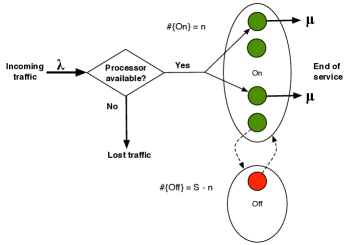
Figure 1: System model for cloud providers.

Within the control of the provider is the ‘resource allocation’ policy, which decides how many servers to run. The objective is to find the optimal number of servers, $n$, that should be switched on in order to optimize the provider’s profit. The extreme values, $n=0$ and $n=S$, correspond to switching respectively off, or on, all available servers.

Unfortunately, because of the random nature of user demand, static policies would under-perform, as servers would be under-utilized when the traffic is low – wasting energy and reducing the provider’s revenues – and overloaded during peak hours, missing the profit opportunities. In order to tackle these issues the provider should be able to dynamically change the number of running servers in response to changes in user demand. The problem is how to do that in a sensible manner.

During the intervals between consecutive policy invocations, the number of running servers remains constant. Those intervals, which will be referred to as ‘observation windows’, are used by the controlling software to collect traffic statistics and obtain current estimates of the average arrival rate ($\lambda$) and service time ($1/\mu$) as well as the squared coefficients of variation of the above values (the variance divided by the square of the mean), $ca^{2}$ and $cs^{2}$ respectively. These values are used by the allocation policy at the next decision epoch.

It is assumed that the time it takes to change the state of a server is negligible compared to the size of the observation windows. That assumption let us neglect the amount of time/energy wasted by servers during reconfigurations. Moreover, in a practical implementation, a decision to switch a server off does not necessarily have to take effect immediately. If a job is being served at that time, it is allowed to complete before the server is turned off.

N.B The assumption that the power up/down operations are instantaneous can be relaxed, at the expenses of complicating the allocation policy. We deliberatively opted not to do so as introducing a short power up/down interval has a little effect on the optimal number of servers to run. On the other hand, if the time it takes to power a server up/down is about the same as the configuration interval (i.e., 10 and 30 minutes), than the energy wasted during system reconfigurations should be explicitly taken into account.

While different metrics can be used to measure the performance of a computing system, as far as the service provider is concerned, the performance of the system is measured by the average revenue, $R$, earned per unit time. That value can be estimated as

$$R=\frac{c}{\mu}T-rP\mbox{,}$$ (1)

where $c/\mu$ is the average charge paid by a customer for having his/her job run, $T$ is the system’s throughput, and $P$ is the total average power consumed by the running servers (servers that are currently switched off do not consume anything).

Please note that, although we make no assumption regarding the relative magnitudes of charges and costs parameters, the most challenging case is when they are close to each other. If the charge for executing a job is much higher than the cost paid by the provider to run a server, one could guarantee a positive (but not optimal) revenue by switching on all servers, regardless of the load. On the other hand, if the charge is smaller than the cost, than it would be better to switch all servers off. Finally, the above model can be easily extended in a number of different ways. For example, one might include the cost for tearing servers up and down, as well as the cost for a smaller mean time between failures (MTBF) of the hardware. However, it is important to to note that the proposed approach can be used in scenarios when the price for electricity is not constant and depends on the time of the day, week, month, etc. In this case, during each reconfiguration a different value for $c$ should be used.

IV Policies

In order to develop a meaningful framework for energy consumption control, it is necessary to have a quantitative model of user demand and service provision. Assuming that jobs enter the system according to an independent Poisson process with rate $\lambda$, we model the number of jobs inside the system, for a fixed number of servers $n$, as the number of jobs in an Erlang loss (or Erlang-B) system with $n$ trunks and traffic intensity $\rho=\lambda/\mu$.

Thus, we can treat the resulting system as an $M/GI/n/n$ queuing model (the ‘M’ stands for Markovian arrivals), which has independent and identically distributed (i.i.d.) service times with a general distribution (the ‘GI’) and independent of the arrival process, $n$ servers, and no extra waiting spaces (e.g., if all servers are busy, further jobs are lost), augmented with the economic parameters introduced in Section III. Since the Erlang-B model is insensitive to the distribution of job sizes, we do not need to worry about the distribution of job lengths. In other words, the blocking probability is independent of the service time distribution beyond its mean; thus, the state probabilities of this system are the same as that of the corresponding purely Markovian $M/M/n/n$ system where the service times are exponentially distributed. This model ignores the time-dependence sometimes found in job arrival processes. However, this time-dependence often tends to be not too important over short time intervals.

When $\rho=n$, the system is critically loaded in the limit, and is said to be in the Quality and Efficiency-Driven (QED) regime, also known as Halfin-Whitt regime [11]. In this paper, we focus on heavily loaded server farms where $\rho\sim n$, as our aim is to switch off servers in excess while serving as many customers as possible. Moreover, we assume that the number of running servers increases if the arrival rate grows, i.e., $n\rightarrow\infty$ as $\lambda\rightarrow\infty$, while the service time distribution does not change with $n$. Under these circumstances, there is a clear separation of time scales [12]: as $n$ increases, arrivals and completions occur more and more quickly (i.e., in a fast time scale), while the experience of individual jobs does not change (i.e., in a slow time scale).

Under the Erlang loss model, the number of jobs inside the system can be modeled as a Birth-and-Death process with a finite state space, $\{0,1,\ldots,n\}$. An arriving job that finds $j$ ($j<n$) jobs being served causes a transition to state $(j+1)$ at rate $\lambda_{j}=\lambda$. A completing job at state $j$ ($j=1,\ldots,n$) causes a transition to state $(j-1)$ at rate $\mu$, and thus jobs leave the system at rate $\mu_{j}=j\mu$. Denote by $p_{j}$ the stationary probability that there are $j$ jobs in the $M/GI/n/n$ queue, $j=0,1,\ldots,n$. After some algebraic manipulations, the balance across the cuts can be expressed in the form

$$p_{j}=\frac{\rho^{j}}{j!}p_{0}\mbox{ .}$$ (2)

Steady-state for this Birth-and-Death process exists if, and only if, Equation (2) can be normalized, i.e., if $\sum^{n}_{j=0}p_{j}=1$. Under this model, the steady-state always exists, and from the normalization condition, we obtain [13]

$$p_{0}=\left[\sum^{n}_{j=0}\frac{\rho^{j}}{j!}\right]^{-1}\mbox{.}$$ (3)

The probability of losing a job, i.e., the probability $p_{n}$ to be in state $n$, is given by the Erlang-B formula

$$p_{n}=B(n,\rho)=\frac{\rho^{n}}{n!}p_{0}\mbox{ .}$$ (4)

Because of the factorial and large power elements, Equation (4) is very difficult to calculate directly from its right-hand side when $n$ and $\rho$ are large. However, it can be computed efficiently using the following iterative scheme [14]

$$\left\{\begin{array}[]{l}B(0,\rho)=1\\ B(n+1,\rho)=\displaystyle{\frac{\rho B(n,\rho)}{n+1+\rho B(n,\rho)}}\end{array}\right.\mbox{.}$$ (5)

If the arrival process is not Poisson, then the insensitivity property is lost, and the appropriate queueing model becomes $G/GI/n/n$, for which there is no exact solution. However, an acceptable approximation for the blocking probability is provided by the formula (see Whitt, [15])

$$p_{n}=B\left(\frac{n}{z},\frac{\rho}{z}\right)\mbox{,}$$ (6)

where $z$ is the asymptotic peakedness of the arrival process, defined as the variance divided by the mean of the steady-state queue length in the associated $G/GI/\infty$ model (see [15] for more details). That value can be computed using the following formula

$$z=1+(ca^{2}-1)\eta{\mbox{,}}$$ (7)

where $\eta$ is defined as

$$\eta=\mu\int_{0}^{\infty}[1-G(t)]^{2}dt{\mbox{,}}$$ (8)

and $G(t)$ is the cumulative distribution function (CDF) of the service time distribution with mean $1/\mu$ and variance $\sigma_{s}^{2}$.

Given the limited amount of information available, evaluating $G(t)$ is very challenging. Thus, we distinguish between three cases:

Case 1: $ca^{2}=1$. The interarrival intervals are exponentially distributed, and $z$ evaluates to 1. Thus, Equation (6) reduces to Equation (4).

Case 2: $ca^{2}\neq 1$ and $cs^{2}=1$. The service times are exponentially distributed, $\eta=1/2$ and therefore $z$ is

$$z=1+\frac{(ca^{2}-1)}{2}\mbox{.}$$ (9)

Case 3: $ca^{2}\neq 1$ and $cs^{2}\neq 1$. We use a normal approximation to solve Equation (7). Denoted by $N(m,\sigma^{2})$ a normal random variable with mean $m$ and variance $\sigma^{2}$. We approximate the distribution $G(t)$ by the distribution of $N(1/\mu,\sigma_{s}^{2})$, and compute the integral in Equation (8) using the Legendre-Gauss integration method.

Finally, since the service time distribution might change over the time, it may be convenient to periodically recompute the peakedness factor. Denoted by $z_{k}$ the peakedness at decision epoch $k$. At time $(k+1)$, the new peakedness can be estimated as

$$z_{k+1}=1+(z_{k}-1)\eta_{k+1}/\eta_{k}\mbox{.}$$ (10)

Having defined the stationary distribution of the number of jobs present, the average number of jobs entering the system (and completing service) per unit time is

$$T=\lambda(1-p_{n})\mbox{,}$$ (11)

with $(1-p_{n})$ being the probability that an incoming job finds an idle server.

The above expressions, together with (5), enable the average revenue $R$ to be computed efficiently and quickly, e.g., $B(100000,\rho)$ can be evaluated in about 0.2 seconds using an Intel Core Duo processor. When that is done for different set of parameter values, it becomes clear that $R$ is a unimodal function of $n$, i.e., it has a single maximum, which might be $n=S$, or $n=0$, see discussion in Section III (this does not depend on the assumption that the electricity cost is constant over the time). We do not have a mathematical proof of this proposition, but have verified it in several numerical experiments. Since the cost for evaluating $R$ is domininated by the computation of Equations (5) and (8) (where the latter has to be computed only once), one can search for the optimal number of servers to run by evaluating $R$ for consecutive values of $n$, stopping either when $R$ starts decreasing or, if that does not happen, when the revenue increase becomes smaller than some value $\epsilon$. This can be justified by arguing that the revenue is a concave function with respect to $n$. Intuitively, the economic benefits of switching on more servers become less and less significant as $n$ increases. On the other hand, the loss of potential revenues become more and more significant as $n$ decreases. Such behavior is an indication of concavity. One can therefore assume that any local maximum reached is, or is close to, the global maximum.

The allocation policy described above, which will be refferred to as ‘Optimal’ policy, requires the evaluation of Equations (5) and (8). It may therefore be desirable to have simpler heuristics that allow decisions to be taken faster and with less information.

IV-A Adaptive Heuristic

Deciding on the number of servers to run requires to balance between the server farm’s utilization and service quality (availability). High utilization is typically obtained at the cost of lower availability. Therefore, it is a common belief that high utilization and good service quality can not coexist. However, the behaviour of large server farms working in QED regime differs from that of Kingman’s Law (i.e., delays/job losses are very common under heavy load) in that service quality is carefully balanced with server efficiency.

Thus, we propose the following ‘Adaptive’ heurisitc. From the statistics collected during a window, estimate the arrival rate, $\lambda$, and average service time, $1/\mu$. For the duration of the next window, allocate the servers according to

$$n=\left\lceil\rho+\beta\sqrt{\rho}\right\rceil\mbox{,}$$ (12)

where the quantity $\beta\sqrt{\rho}$ is used for dealing with stochastic variability, and $-1\leq\beta\leq 1$.

IV-B Predictive Heuristic

One can observe that the previously discussed policies simply adapt to the changes in user demand by assuming that the traffic during the next window will be the same as that of the previous window. The realism of that assumption can be disputed, as the load typically follows certain patterns (daily, weekly, etc.). Thus, is might be desirable to design a policy which tries to predict the user demand.

Denoted by $\rho_{k}$ is the estimated load at window $k$. Instead of simply adapting to the observed load and assuming that $\rho_{k}=\rho_{k+1}$, one can try to forecast and estimate what $\rho_{k+1}$ will be using the historical data. Thus, a simple and efficient heuristic using a double exponential smoothing to estimate the future arrival rate can be employed. For any time period $k$, the smoothed value $S_{k}$ is found by solving the following system of equations

$$\left\{\begin{array}[]{l}S_{k}=\alpha\lambda+(1-\alpha)(S_{k-1}+b_{k-1})\\ b_{k}=\gamma(S_{k}-S_{k-1})+(1-\gamma)b_{k-1}\\ \end{array}\right.\mbox{.}$$ (13)

The first equation adjusts the smoothed value $S_{k}$ adding $b_{k-1}$ to the last smoothed value, $S_{k-1}$, while the second equation updates the trend. In this work we used the least squared method in order to find the best values for $\alpha$ and $\gamma$.

Having computed the smoothed and the trend values at time $k$, the forecast for the arrival rate at time $(k+1)$, $\lambda_{k+1}^{F}$, is computed as $\lambda_{k+1}^{F}=S_{k}+b_{k}\mbox{.}$

V Server Power Usage Estimation

The amount of electricity drawn by servers depends on several factors. Moreover, realistic cost models should take into account wasted energy such as power conversion losses and the power used for cooling purposes. Different algorithms can be employed to estimate the energy requirements of a data center, the simplest one assuming that the power usage of a server is constant, while the most complex models using also disk metrics gathered from some operating system tools such as iostat, in addition to the CPU utilization, or performance counters [16].

Since most of the Cloud applications are most likely web applications, we conducted an experiment aiming at finding the dependency between the energy consumption and CPU utilization for a common web application. In order to avoid biased applications, i.e., with high CPU consumption per job, we have chosen Wordpress as a study case. This application runs on top of the LAMP stack (i.e., Linux, Apache, MySQL and PHP), and thus represents a significant fraction of the applications running not only in the Cloud but in the Internet as well. Moreover, Wordpress jobs are not completely CPU bound, as the application uses a database as a backend, whose operations are I/O bound. Unfortunately, the default configuration of LAMP is far from being optimized for high throughput under heavy load. Therefore, we had to perform a number of tune ups, including installing XCache – which caches the compiled PHP code, thus preventing re-compiling the same code for every arrival – and tuning the TCP stack, the Linux kernel and the Apache configuration.

The server was hosted on a machine with Dual Xeon Dual Core CPUs running at 2.8 Ghz, 2 Gb of RAM, 7200 RPM hard drive and 1 Gbps network card. The power consumption was measured every minute in the presence of an increasing workload, which was generated by Tsung 1.3.2. The workload consisted of clients arriving according to a Poisson process at an increasing rate. Each client replayed a prerecorded session, which included checking the front page, browsing the posts with some specific tags, as well as searching in the blog. Surprisingly, most of the HTTP requests were serving dynamic content, as the static content, which consisted from CSS files and JavaScript libraries, was cached on client’s side after the first client’s request.

Figure 2: Measured energy consumption.

Figure 2 demonstrates the relationship between power consumption and CPU utilization. In the idle mode, the energy consumption stayed at the steady 140 W. As shown in Figure 2, the power consumption grows linearly with the increase of CPU utilization. Noise in the power consumption can be attributed to noise in the CPU utilization due the irregularity in the request traffic. Besides, the fluctuations in the CPU utilization require dynamic usage of the cooling fans, which in turn amplifies the fluctuations in the power consumption. The power consumption peeks at 220 W when the CPU utilization reaches values higher than 375%. Due to the lack of space, we do not present the behavior of the response time, which stayed under one second for loads up to 70%.

Therefore, the average power consumed by a data center per unit time, $P$, can be estimated as

$$P=ne_{1}+\bar{m}(e_{2}-e_{1})\mbox{,}$$ (14)

where $e_{1}$ is the energy consumed per unit time by idle servers, $e_{2}$ is the energy drawn by each busy server, and $\bar{m}$ is the average number of servers running jobs ($\bar{m}\leq n$)

$$\bar{m}=\left\lceil\frac{T}{\mu}\right\rceil\mbox{.}$$ (15)

We have carried out some tests with some other models, and found that the estimate given by Equation (14) gets within 10% of the one using performance counters.

VI Performance Evaluation

Various experiments were carried out, with the aim of evaluating how the proposed policies affect the maximum achievable revenues. We assume a server farm with a Power Usage Effectiveness (PUE) of 1.7 [5]. The PUE is one of the metrics used to measure the efficiency of data centers, and it is computed as the ratio between the total facility power and the IT equipment power. Also, to reduce the number of variables, if not otherwise stated, the following features and assumptions were held fixed:

• The data center is composed of 25,000 machines, configured as in Section V. Therefore, $S=100,000$.

• The power consumption of each Xeon machine ranges between 140 and 220 W, see Figure 2. In other words, each server (e.g., core, fans, disk and network interface) has a direct consumption between 35 and 55 W. Since the server farm has a PUE factor of 1.7, the minimum and maximum power consumption are approximately $e_{1}$ = 59 and $e_{2}$ = 94 W per server.

• The cost for electricity, $r$, is 0.1 $ per kWh [17].

• The average job size, $1/\mu$, is set to 50 minutes.

• Completed jobs generate an amount of income of 0.085 $/hour. Charges are proportional to the job length, and therefore each job is worth on average 0.071 $.

• Jobs are not completely CPU bound. Instead, when a server is busy, the average CPU utilization is 70%. In other words, busy servers draw 69.58 Wh, and thus each job costs, for electricity, 0.0058 $ on average.

To make the results more realistic we take indirect costs into account as well. These include the cost of capital and equipment amortization (servers as well as power generators, transformers, UPS systems, etc.), and account for twice the cost of consumed electricity.

The first experiment is purely numerical. In Figure 3 we examine how the number of running servers affects the average earned revenue per unit time under different loading conditions. The potential offered load is increased from 30% to 90% by increasing the rate at which new jobs enter the system, from 36,000 to 108,000 jobs per hour.

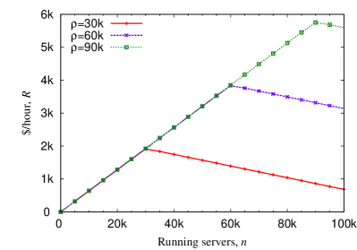
Figure 3: Revenue as function of the running servers.

The figure illustrates the following points:

1. In each case there is an optimal number of servers that should be switched on;

2. The heavier is the load, the higher is the optimal number of servers as well as the maximum achievable revenue;

3. When $n>n_{opt}$, the system under-performs because the cost of running idle servers erodes revenues;

4. When $n<n_{opt}$, the system under-performs because it misses potential revenues.

Next, we evaluate the performance of the proposed policies via event-driven simulation. For comparison reasons, two versions of the ‘Static’ policy, a policy which runs always the same amount of servers, is also displayed. One runs $n=S/2=50,000$ servers, while the other $n=S=100,000$. We vary the load between 5% and 99.5% by varying the arrival rate, i.e., $\lambda=6,000,\ldots,119,400$ jobs/hour. Each point in the figure represents one run lasting 264 hours (i.e., 11 days), while reconfigurations occur every 2 hours. During each run, between 1.6 (low load) and 35 million (high load) jobs arrive into the system (the number of jobs admitted into the system is a bit smaller under heavy load). Samples of achieved revenues are collected approximately every 24 hours and are used at the end of each run to compute the corresponding 95% confidence interval, which is calculated using the Student’s t-distribution.

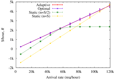
Figure 4: Observed revenues for different policies. Markovian scenario.

The most notable feature of the graph plotted in Figure 4 is that the performance of the ‘Static’ policies produce negative revenues under light load (because of the servers running idle), while the one with parameter $n=S/2$ performs poorly when the load increases, because too many jobs are lost. On the other hand, the ‘Adaptive’ heuristic (with parameter $\beta=0.2$) produces revenues that grow with the offered load, and almost as high as those obtained by the more computationally expensive ‘Optimal’ algorithm. This suggests that the ‘Adaptive’ heuristic might be a suitable choice for practical implementation.

Figure 4 does not allow to see a comprehensive picture, but it shows that the policies we propose perform better than the static ones, it does not provide any insight about the optimality of the algorithms. Therefore, in Figure 5 we show the ratio between busy and running servers: a value close to 1 means that the policy performs very well, while a value close to 0 means that the algorithm does not behave properly. The figure shows that the ‘Adaptive’ heuristic is always very close to 1. The percentage of lost jobs obtained by those policies is always very low, thus ensuring a good user experience.

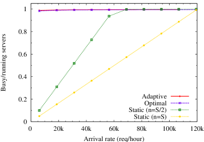
Figure 5: Ratio between busy and running servers.

Finally, Figure 6, which depicts the average power consumption, clearly shows that the dynamic policies run servers only when needed, thus reducing the electricity bill and improving the provider’s profits.

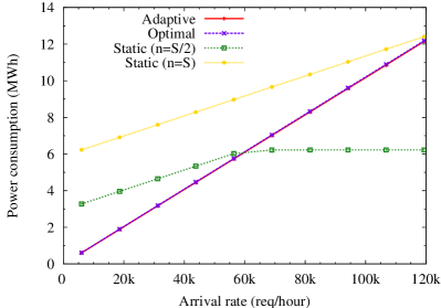
Figure 6: Average power consumption for different policies.

Next, we depart from the assumption that the traffic is Markovian in order to evaluate the effect of interarrival and service time variability on performance. The average values are kept the same as before, however both the interarrival and service times are generated according to a Log-Normal distribution. The corresponding squared coefficient of variation are $ca^{2}=2$ and $cs^{2}=20$. The high variability in job size distribution was deliberately chosen to reflect the different kind of cloud users.

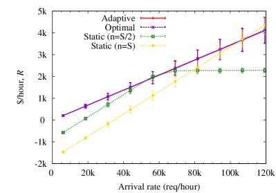
Figure 7: Observed revenues for different policies, $ca^{2}=2$ and $cs^{2}=20$.

It is legitimate to expect the performance to deteriorate when the traffic variability increases, since the system becomes less predictable and it is more difficult to choose the best $n$. In fact, Figure 7 shows that the achieved revenues are indeed lower than those achieved when the traffic is Markovian.

In the next series of the experiments we evaluate the performance of the proposed policies under non stationary loading conditions. Unfortunately, there is no publicly available data describing the demand for Cloud resources, and thus we extrapolated it from the available Wikipedia traces [18]. Therefore the increase/decrease in the Wikipedia traffic would correlate with the general increase/decrease of the request rate for the resources. The arrival rate behavior has a general trend, with monthly, weekly and daily patterns, as well as unexpected spikes, which are hard to predict. We believe that such a workload is unbiased and thus will not provide advantages for any specific approach. We assume that jobs enter the system arriving according to a Poisson process with a certain rate $\lambda$ which changes every hour, while the system is reconfigured every 30 minutes.

As it has been pointed out above, the QED algorithm performs almost as good as the optimal allocation policy. Therefore, the next set of experiments are conducted using the QED algorithm. We evaluate the performance of QED with adaptive and predictive heuristic, and, for comparison reasons, we also include a static allocation policy that runs all the available servers, and an ‘Oracle’ policy that knows the exact value of $\lambda$ for the next time interval, and thus allocates the optimal number of servers. Figure 8 shows that the static allocation policy achieves 55%-80% utilization, while the dynamic policies use a smaller amount of servers for handling the load, thus the achieved utilization is significantly higher.

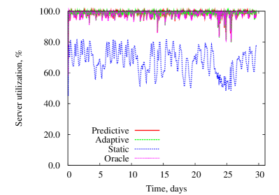
Figure 8: Data center utilization.

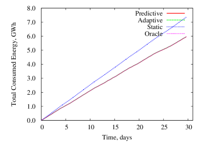
Figure 9: Cumulative power consumption measured over one month

Since fewer servers are needed for handling the same load, the resulting power consumption is also markedly smaller [fig. 9]. It is interesting to observe that despite the difference in the prediction mechanisms, all QED variations demonstrate almost identical results in terms of achieved cumulative revenue, see Figure 10. This can be attributed to the fact the load fluctuation within the reconfiguration intervals is rather small and hard to predict.

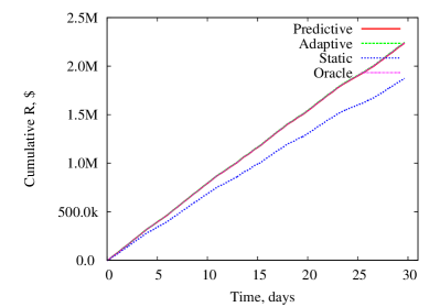
Figure 10: Cumulative revenue measured over one month.

VII Conclusions

We have introduced and throughly evaluated easily implementable policies for dynamically adaptable cloud provision. We have demonstrated that decisions, such as how many servers are powered on, can have a significant effect on the revenue earned by the provider. Moreover, those decisions are affected by the contractual obligations between clients and provider. The experiments we have carried out showed that the proposed polices work well under different traffic conditions, and that the ‘Adaptive’ heuristic would be a good candidate for practical implementation.

Possible directions for future research include taking into account the time and energy consumed during systems reconfigurations, trade offs between the number of running servers and the frequency of the CPUs, and the power consumed by the networking equipment (i.e., switches).

References

- [1] J. Hamilton, “Data Center Efficiency Best Practices,” Amazon Web Services, April 2009. [Online]. Available: www.mvdirona.com/jrh/TalksAndPapers/JamesHamilton˙Google2009.pdf
- [2] M. Pedram, “Energy-efficient computing,” 2009. [Online]. Available: http://atrak.usc.edu/~massoud/Talks/Pedram-DASS-09.pdf
- [3] L. A. Barroso and U. Hölzle, “The case for energy-proportional computing,” Computer, vol. 40, no. 12, pp. 33–37, 2007.
- [4] Windows 7 Power Management Whitepaper, Microsoft, April 2009.
- [5] A. Greenberg, J. Hamilton, D. A. Maltz, and P. Patel, “The Cost of a Cloud: Research Problems in Data Center Networks,” SIGCOMM Comput. Commun. Rev., vol. 39, no. 1, pp. 68–73, January 2009.
- [6] E. M. Elnozahy, M. Kistler, and R. Rajamony, “Energy-efficient server clusters,” in In Proceedings of the 2nd Workshop on Power-Aware Computing Systems, 2002, pp. 179–196.
- [7] V. Sharma, A. Thomas, T. Abdelzaher, K. Skadron, and Z. Lu, “Power-aware qos management in web servers,” in RTSS ’03: Proceedings of the 24th IEEE International Real-Time Systems Symposium. Washington, DC, USA: IEEE Computer Society, 2003, p. 63.
- [8] Y. Chen, A. Das, W. Qin, A. Sivasubramaniam, Q. Wang, and N. Gautam, “Managing server energy and operational costs in hosting centers,” SIGMETRICS Perform. Eval. Rev., vol. 33, no. 1, pp. 303–314, 2005.
- [9] D. N. M. Hedwig, S. Malkowski, “Taming energy costs of large enterprise systems through adaptive provisioning.” in ICIS, 2009.
- [10] A. Qureshi, R. Weber, H. Balakrishnan, J. Guttag, and B. Maggs, “Cutting the Electric Bill for Internet-Scale Systems,” in ACM SIGCOMM, Barcelona, Spain, August 2009.
- [11] S. Halfin and W. Whitt, “Heavy-Traffic Limits for Queues with Many Exponential Servers,” Operations Research, vol. 29, May-June 1981. [Online]. Available: http://www.columbia.edu/~ww2040/HalfinWW1981.pdf
- [12] W. Whitt, Stochastic-Process Limits. Springer-Verlag, 2002.
- [13] I. Mitrani, Probabilistic Modelling. Cambridge University Press, 1998.
- [14] O. Hudousek, “Evaluation of the Erlang-B formula,” in Proceedings of RTT 2003, 2003.
- [15] W. Whitt, “Heavy Traffic Approximations for Service Systems with Blocking,” AT&T Bell Laboratories Technical Journal, vol. 63, May-June 1984.
- [16] S. Rivoire, P. Ranganathan, and C. Kozyrakis, “A Comparison of High-Level Full-System Power Models,” in Proceedings of the Workshop on Power Aware Computing and Systems (HotPower ’08), December 2008.
- [17] Nebraska Energy Office, “Electricity Rate Comparison by State,” December 2009. [Online]. Available: http://www.neo.ne.gov/statshtml/115.htm
- [18] G. Urdaneta, G. Pierre, and M. van Steen, “Wikipedia workload analysis for decentralized hosting,” Comput. Netw., vol. 53, no. 11, pp. 1830–1845, 2009.