Quark-Model Baryon-Baryon Interaction Applied to the Neutron-Deuteron Scattering (III)

Abstract

The low-energy breakup differential cross sections of the neutron-deuteron ($nd$) scattering are studied by employing the energy-independent version of the quark-model baryon-baryon interaction fss2. This interaction reproduces almost all the breakup differential cross sections predicted by the meson-exchange potentials for the neutron incident energies $E_{n}\leq 65$ MeV. The space star anomaly of 13 MeV $nd$ scattering is not improved even in our model. Some overestimation of the breakup differential cross sections at $E_{n}=22.7$ - 65 MeV implies that systematic studies of various breakup configurations are necessary both experimentally and theoretically.

205

1 Introduction

The three-nucleon ($3N$) system is a good place to study the underlying nucleon-nucleon ($NN$) interaction, since many techniques to solve the system exactly are well developed nowadays.[1, 2] Ample experimental data are already accumulated especially for the low-energy neutron-deuteron ($nd$) and proton-deuteron ($pd$) scattering and extensive studies to detect the $3N$ force have been carried out based on the modern meson-exchange potentials,[3, 4] and more recently, on the chiral effective field theory.[5, 6] Most of the researches to such a direction are concerned with higher energies than 100 MeV for the nucleon incident energy $E_{n}$ in the laboratory (lab) system, since the $3N$ force effect is expected to be revealed more prominently than in the low energies.[3] On the other hand, the discrepancies of various $3N$ observables between the theory and experiment in the $E_{n}\leq 65$ MeV region, are not resolved even by the recent accurate treatment of the Coulomb force.[7, 8, 9] This is particularly true for the nucleon-induced deuteron breakup processes. It is therefore worth while reexamining the $NN$ interaction itself if the present-day realistic force is the most appropriate one to start with.

In previous papers,[10, 11] referred to as I and II hereafter, we have applied the quark-model (QM) baryon-baryon interaction fss2 to the neutron-deuteron ($nd$) elastic scattering. This interaction model, fss2, describes available $NN$ data in a comparable accuracy with the modern meson-exchange potentials.[12] By eliminating the inherent energy dependence of the resonating-group kernel, fss2 was found to yield a nearly correct triton binding energy, the $S$-wave $nd$ scattering length, and the low-energy eigenphase shifts without reinforcing it with the three-body force.[13, 14, 15] The predicted elastic differential cross sections have sufficiently large cross section minima at $E_{n}=35\,\hbox{-}\,65$ MeV and $\theta_{\rm cm}=130^{\circ}\,\hbox{-}\,135^{\circ}$, in contrast to the predictions by the standard meson-exchange potentials.[10] The so-called $A_{y}$ puzzle at low-energies $E_{n}\leq 25$ MeV is largely improved in this model.[11] In this paper, we continue these studies by examining the $3N$ breakup processes with various decaying kinematics for the energy range $E_{n}\leq 65$ MeV. The main motivation is to find if the quite different off-shell properties, originating from the strong nonlocality of the QM baryon-baryon interaction, give some influence to the $3N$ breakup differential cross sections. In contrast to the elastic scattering amplitude, the breakup amplitude covers a wide momentum region of the three-body phase space. It will be found unfortunately that the fss2 gives predictions similar to the meson-exchange potentials and does not improve much the discrepancies between the theory and the experiment.

The organization of this paper is as follows. In $\S\,2.1$, the formulation of the breakup differential cross sections is given in terms of the direct breakup amplitude. Various kinematical configurations for the three-body decay are introduced in $\S\,2.2$. A minimal description of the three-nucleon breakup kinematics is given in Appendix A. The isospin factors for the breakup amplitudes are derived in Appendix B. The comparison with the experimental data is presented in $\S\,3$ for energies $E_{n}=8,~{}10.3,~{}10.5,~{}13,~{}16,~{}19,~{}22.7$ and 65 MeV. The difference from the predictions by meson-exchange potentials are discussed in detail. We close this paper with a summary of this series of investigations in $\S\,4$.

2 Formulation

2.1 Breakup differential cross sections

Following the notation of Refs. PREP, I and II, the three-body breakup amplitude is given by

$$U_{0}|\phi\rangle=(1+P)T|\phi\rangle=(1+P)t\widehat{Q}|\phi\rangle\ .$$ (1)

In order to derive the breakup differential cross sections, we start from the Fermi’s golden rule

$$d\,N=\frac{2\pi}{\hbar}|\langle{\boldsymbol{p}}{\boldsymbol{q}}|U_{0}|\phi\rangle|^{2}\int^{\infty}_{0}p^{2}\,d\,p~{}\delta(E-E_{pq})~{}q^{2}\,d\,q~{}d\,\widehat{{\boldsymbol{p}}}~{}d\,\widehat{{\boldsymbol{q}}}\ ,$$ (2)

and divide it by the incident flux $j=(3\hbar q_{0}/2M)/(2\pi)^{3}$. Here, $E_{pq}=(\hbar^{2}/M)(p^{2}+3q^{2}/4)$, $M$ is the nucleon mass, and $q_{0}$ is the incident momentum related to the energy, $E=(3\hbar^{2}/4M){q_{0}}^{2}+\varepsilon_{d}$, in the center-of-mass (cm) system. We obtain in the cm system

$$\frac{d^{5}\,\sigma}{d\,\widehat{{\boldsymbol{p}}}~{}d\,\widehat{{\boldsymbol{q}}}~{}d\,q} = \frac{1}{j}\frac{d\,N}{d\,\widehat{{\boldsymbol{p}}}~{}d\,\widehat{{\boldsymbol{q}}}~{}d\,q}=(2\pi)^{4}\frac{2M}{3\hbar^{2}}\frac{1}{q_{0}}\int^{\infty}_{0}p^{2}\,d\,p~{}\delta(E-E_{pq})~{}q^{2}~{}|\langle{\boldsymbol{p}}{\boldsymbol{q}}|U_{0}|\phi\rangle|^{2}$$ (3)

$$= (2\pi)^{4}\left(\frac{2M}{3\hbar^{2}}\right)^{2}\frac{3}{4}\frac{p_{0}q^{2}}{q_{0}}\sum_{\Gamma}|\langle{\boldsymbol{p}}{\boldsymbol{q}}\Gamma|U_{0}|\phi\rangle_{0}|^{2}\ ,$$

where Eq. I(2.88) is used to perform the $p$-integral. In Eq. (3), $\Gamma=\Gamma_{\sigma}\Gamma_{\tau}$ is the spin-isospin quantum numbers in the $LS$-coupling scheme and the subscript 0 in the matrix element implies the on-shell condition $|{\boldsymbol{p}}|=p_{0}=\sqrt{(3/4)({q_{M}}^{2}-q^{2})}$ with $q_{M}=\sqrt{{q_{0}}^{2}-{\kappa_{d}}^{2}}$. Here, $\kappa_{d}$ is related to the deuteron binding energy $|\varepsilon_{d}|$ through $|\varepsilon_{d}|=(3\hbar^{2}/4M){\kappa_{d}}^{2}$. In this paper, we use the notation $\Gamma_{\sigma}=(s{\scriptstyle\frac{1}{2}})SS_{z}$ and $\Gamma_{\tau}=(t{\scriptstyle\frac{1}{2}}){\scriptstyle\frac{1}{2}}T_{z}$ to specify the quantum numbers in the $LS$-coupling scheme: i.e.,

$$|{\boldsymbol{p}},{\boldsymbol{q}};123\rangle=\sum_{\gamma}|p,q,\gamma\rangle~{}\langle\gamma|\widehat{{\boldsymbol{p}}},\widehat{{\boldsymbol{q}}};123\rangle\ ,$$

$$\langle\widehat{{\boldsymbol{p}}},\widehat{{\boldsymbol{q}}};123|\gamma\rangle=\left[Y_{(\lambda\ell)L}(\widehat{{\boldsymbol{p}}},\widehat{{\boldsymbol{q}}})~{}\xi_{\Gamma_{\sigma}}(12,3)\right]_{JJ_{z}}~{}\eta_{\Gamma_{\tau}}(12,3)\ ,$$ (4)

with $\gamma=[(\lambda\ell)L\Gamma_{\sigma}]JJ_{z};\Gamma_{\tau}$, and $\xi_{\Gamma_{\sigma}}$ and $\eta_{\Gamma_{\tau}}$ being the three-particle spin and isospin wave functions, respectively. In Eq. (4), $Y_{(\lambda\ell)LM}(\widehat{{\boldsymbol{p}}},\widehat{{\boldsymbol{q}}})=[Y_{\lambda}(\widehat{{\boldsymbol{p}}})Y_{\ell}(\widehat{{\boldsymbol{q}}})]_{LM}$ are the angular functions. For the initial state, we use channel-spin representation as for the elastic scattering. We take the sum of Eq. (3) over all the spin and isospin quantum numbers and divide by the initial spin multiplicity 6. The selection of the detected particles in the final state is controlled by the isospin projection operator ${\cal O}_{\tau}$, the explicit form of which will be specified later. The breakup differential cross sections of the $nd$ scattering are therefore calculated from

$$\frac{d^{5}\,\sigma}{d\,\widehat{{\boldsymbol{p}}}~{}d\,\widehat{{\boldsymbol{q}}}~{}d\,q}=(2\pi)^{4}\left(\frac{2M}{3\hbar^{2}}\right)^{2}\frac{3}{4}\frac{p_{0}q^{2}}{q_{0}}\frac{1}{6}\sum_{\Gamma}\sum_{S_{c}S_{cz}}|\langle{\boldsymbol{p}}{\boldsymbol{q}}\Gamma|{\cal O}_{\tau}(1+P)T|\phi_{{\boldsymbol{q}}_{0}};S_{c}S_{cz}\rangle_{0}|^{2}\ .$$

(5)

Let us first consider the spin-isospin sum $I=\sum_{\Gamma}|\langle{\boldsymbol{p}}{\boldsymbol{q}}\Gamma|(1+P)f\rangle|^{2}$ by neglecting the initial spin quantum numbers for the time being. The effect of the permutation ${P_{(123)}}^{\alpha}$ in $(1+P)=\sum^{3}_{\alpha=1}{P_{(123)}}^{\alpha}$ is defined by

$$\langle{\boldsymbol{p}}{\boldsymbol{q}}|{P_{(123)}}^{\alpha}f\rangle\equiv{P_{(123)}}^{\alpha}f({\boldsymbol{p}},{\boldsymbol{q}})=f({\boldsymbol{p}}_{\alpha},{\boldsymbol{q}}_{\alpha})\ ,$$ (6)

if the function $f({\boldsymbol{p}},{\boldsymbol{q}})$ does not contain the spin-isospin degree of freedom. In fact, we should use

$$\langle{\boldsymbol{p}}{\boldsymbol{q}}\Gamma|{P_{(123)}}^{\alpha}f\rangle=\langle\Gamma|{P^{(\sigma\tau)}_{(123)}}^{\alpha}f({\boldsymbol{p}}_{\alpha},{\boldsymbol{q}}_{\alpha})\rangle\ ,$$ (7)

where $P^{(\sigma\tau)}_{(123)}$ is the permutation operator in the spin-isospin space and the bra-ket notation is used for the spin-isospin degree of freedom. Using these notations and the completeness relationship in the spin-isospin space, $\sum_{\Gamma}|\Gamma\rangle\langle\Gamma|=1$, we find

$$I=\sum^{3}_{\alpha,\beta=1}\langle f({\boldsymbol{p}}_{\alpha},{\boldsymbol{q}}_{\alpha})|{P^{(\sigma\tau)}_{(123)}}^{3-\alpha}{P^{(\sigma\tau)}_{(123)}}^{\beta}|f({\boldsymbol{p}}_{\beta},{\boldsymbol{q}}_{\beta})\rangle\ .$$ (8)

Here we separate the $\alpha$, $\beta$ sum into the diagonal part ($\alpha=\beta$) and the off-diagonal part ($\alpha\neq\beta$). In the off-diagonal part, we specify $\alpha$ and $\beta$ by the cyclic permutations of (123) ($(\alpha\beta\gamma)$=(123)-cyclic). For these terms, the $\alpha$-$\beta$ term and the $\beta$-$\alpha$ term are complex conjugate to each other. Thus we obtain

$$I=\sum^{3}_{\alpha=1}\langle f({\boldsymbol{p}}_{\alpha},{\boldsymbol{q}}_{\alpha})|f({\boldsymbol{p}}_{\alpha},{\boldsymbol{q}}_{\alpha})\rangle+2\sum^{\prime}_{(\alpha\beta\gamma)}{\rm Re}\,\langle f({\boldsymbol{p}}_{\alpha},{\boldsymbol{q}}_{\alpha})|P^{(\sigma\tau)}_{(123)}|f({\boldsymbol{p}}_{\beta},{\boldsymbol{q}}_{\beta})\rangle\ ,$$ (9)

where $\sum^{\prime}$ implies the sum over the three cyclic permutations of $(\alpha\beta\gamma)=(123)$.

The extension to $I=\sum_{\Gamma}|\langle{\boldsymbol{p}}{\boldsymbol{q}}\Gamma|{\cal O}_{\tau}(1+P)f\rangle|^{2}$, incorporating the isospin projection operator ${\cal O}_{\tau}$, is rather easy. Here, ${\cal O}_{\tau}$ is specified as

$${\cal O}^{pp} = \frac{1+\tau_{z}(1)}{2}\frac{1+\tau_{z}(2)}{2}\ \ ,\qquad{\cal O}^{nn}=\frac{1-\tau_{z}(1)}{2}\frac{1-\tau_{z}(2)}{2}\ ,$$

$${\cal O}^{pn} = \frac{1+\tau_{z}(1)}{2}\frac{1-\tau_{z}(2)}{2}\ \ ,\qquad{\cal O}^{np}=\frac{1-\tau_{z}(1)}{2}\frac{1+\tau_{z}(2)}{2}\ ,\$$ (10)

depending on the species of particles 1 and 2 detected. We use ${{\cal O}_{\tau}}^{2}={\cal O}_{\tau}$ and the notation $\langle{\boldsymbol{p}}{\boldsymbol{q}}\Gamma|f\rangle=f_{\Gamma}({\boldsymbol{p}},{\boldsymbol{q}})$. Then, by defining

$${\cal O}^{\alpha\beta}_{\tau}=\left(P^{\tau}_{(123)}\right)^{3-\alpha}{\cal O}_{\tau}\left(P^{\tau}_{(123)}\right)^{\beta}\qquad(={{\cal O}^{\beta\alpha}_{\tau}}^{\dagger})\ ,$$ (11)

we obtain

$$I = \sum^{3}_{\alpha=1}\sum_{\widetilde{\Gamma},\Gamma}f^{*}_{\widetilde{\Gamma}}({\boldsymbol{p}}_{\alpha},{\boldsymbol{q}}_{\alpha})\,\langle\widetilde{\Gamma}|{\cal O}^{\alpha\alpha}_{\tau}|\Gamma\rangle\,f_{\Gamma}({\boldsymbol{p}}_{\alpha},{\boldsymbol{q}}_{\alpha})$$ (12)

$$+2\sum^{\prime}_{(\alpha\beta\gamma)}\sum_{\widetilde{\Gamma},\Gamma}{\rm Re}\left\{f^{*}_{\widetilde{\Gamma}}({\boldsymbol{p}}_{\alpha},{\boldsymbol{q}}_{\alpha})\,\langle\widetilde{\Gamma}|P^{\sigma}_{(123)}{\cal O}^{\alpha\beta}_{\tau}|\Gamma\rangle\,f_{\Gamma}({\boldsymbol{p}}_{\beta},{\boldsymbol{q}}_{\beta})\right\}\ .$$

The spin-isospin factors in Eq. (12) are calculated by separating the spin-isospin state $|\Gamma\rangle$ to the spin and isospin parts, $|\Gamma\rangle=|\Gamma_{\sigma}\rangle|\Gamma_{\tau}\rangle$. We find

$$\langle\widetilde{\Gamma}|{\cal O}^{\alpha\alpha}_{\tau}|\Gamma\rangle=\delta_{\widetilde{S},S}\,\delta_{\widetilde{s},s}~{}\langle\widetilde{\Gamma_{\tau}}|{\cal O}^{\alpha\alpha}_{\tau}|\Gamma_{\tau}\rangle\ ,$$

$$\langle\widetilde{\Gamma}|P^{\sigma}_{(123)}{\cal O}^{\alpha\beta}_{\tau}|\Gamma\rangle=\delta_{\widetilde{S},S}\,(-1)^{1+s}X^{S}_{\widetilde{s},s}~{}\langle\widetilde{\Gamma_{\tau}}|{\cal O}^{\alpha\beta}_{\tau}|\Gamma_{\tau}\rangle\ ,$$ (13)

where $\widetilde{\Gamma}_{\sigma}=(\widetilde{s}{\scriptstyle\frac{1}{2}})\widetilde{S}\widetilde{S}_{z}$ and $\widetilde{\Gamma}_{\tau}=(\widetilde{t}{\scriptstyle\frac{1}{2}}){\scriptstyle\frac{1}{2}}T_{z}$, and Eq. (77) is used for the spin part. We also extend the definition in Eq. (77) for the spin part to the isospin part as in Eq. (84). Using the definition of $X^{\tau(\alpha\beta)}_{\widetilde{t},t}$ in Eq. (84), we can write the matrix elements in Eq. (13) as

$$\langle\widetilde{\Gamma}|{\cal O}^{\alpha\alpha}_{\tau}|\Gamma\rangle=\delta_{\widetilde{S},S}\,\delta_{\widetilde{s},s}~{}X^{\tau(\alpha\alpha)}_{\widetilde{t},t}\ ,$$

$$\langle\widetilde{\Gamma}|P^{\sigma}_{(123)}{\cal O}^{\alpha\beta}_{\tau}|\Gamma\rangle=\delta_{\widetilde{S},S}\,(-1)^{1+s}X^{S}_{\widetilde{s},s}~{}(-1)^{1+t}X^{\tau(\alpha\beta)}_{\widetilde{t},t}\ ,$$ (14)

for $(\alpha\beta\gamma)=$ a cyclic permutation of (123). Thus we find

$$I = \sum^{3}_{\alpha=1}\sum_{\widetilde{\Gamma},\Gamma}\delta_{\widetilde{S},S}\,\delta_{\widetilde{s},s}\,X^{\tau(\alpha\alpha)}_{\widetilde{t},t}~{}f^{*}_{\widetilde{\Gamma}}({\boldsymbol{p}}_{\alpha},{\boldsymbol{q}}_{\alpha})\,f_{\Gamma}({\boldsymbol{p}}_{\alpha},{\boldsymbol{q}}_{\alpha})$$ (15)

$$+\sum^{\prime}_{(\alpha\beta\gamma)}\sum_{\widetilde{\Gamma},\Gamma}\delta_{\widetilde{S},S}\,(-2)X^{S}_{\widetilde{s},s}\,X^{\tau(\alpha\beta)}_{\widetilde{t},t}~{}{\rm Re}\left\{f^{*}_{\widetilde{\Gamma}}({\boldsymbol{p}}_{\alpha},{\boldsymbol{q}}_{\alpha})\,f_{\Gamma}(-{\boldsymbol{p}}_{\beta},{\boldsymbol{q}}_{\beta})\right\}\ .$$

where the generalized Pauli principle $(-1)^{s+t+\lambda}=-1$ is used for the two-nucleon part of $f_{\Gamma}(-{\boldsymbol{p}}_{\beta},{\boldsymbol{q}}_{\beta})$. The isospin factors $X^{\tau(\alpha\beta)}_{\widetilde{t},t}$ are explicitly given in Appendix B.

We assign the direct breakup amplitude to $f_{\Gamma}({\boldsymbol{p}},{\boldsymbol{q}})$ in Eq. (15) through

$$f_{\Gamma,S_{c}S_{cz}}({\boldsymbol{p}},{\boldsymbol{q}})=-(2\pi)^{2}\left(\frac{2M}{3\hbar^{2}}\right)\langle{\boldsymbol{p}}{\boldsymbol{q}}\Gamma|T|\phi_{{\boldsymbol{q}}_{0}};S_{c}S_{cz}\rangle_{0}\ ,$$ (16)

with $T=t\widehat{Q}$. The partial wave decomposition is given by

$$f_{\Gamma,S_{c}S_{cz}}({\boldsymbol{p}},{\boldsymbol{q}}) = (4\pi)\sum^{\prime}_{\gamma,\ell^{\prime},JJ_{z}}f^{({\rm db})J}_{\gamma,(\ell^{\prime}S_{c})}(q)\sum_{M}\langle LMSS_{z}|JJ_{z}\rangle\,Y_{(\lambda\ell)LM}(\widehat{{\boldsymbol{p}}},\widehat{{\boldsymbol{q}}})$$ (17)

$$\times\sum_{m^{\prime}}\langle\ell^{\prime}m^{\prime}S_{c}S_{cz}|JJ_{z}\rangle\,Y^{*}_{\ell^{\prime}m^{\prime}}(\widehat{{\boldsymbol{q}}}_{0})\ ,$$

where the prime on the sum implies that we take all the orbital angular momentum sum for the $LS$ coupling scheme of $\gamma$; i.e., the sum over only $(\lambda\ell)L$ with $\gamma=[(\lambda\ell)L\Gamma_{\sigma}]JJ_{z};\Gamma_{\tau}$. (Note the extra $(4\pi)$ factor for the scattering amplitude.) It is convenient to define

$$\widehat{Q}^{(\ell S_{c})J}_{i\mu\gamma}=\sum_{(\ell^{\prime}S^{\prime}_{c})}\widetilde{Q}^{(\ell^{\prime}S^{\prime}_{c})J}_{i\mu\gamma}\,f^{J}_{(\ell^{\prime}S^{\prime}_{c})(\ell S_{c})}\ ,$$ (18)

by the solutions, $\widetilde{Q}_{i\mu\gamma}={p_{i}}^{2}\omega_{i}q_{\mu}\sqrt{\omega_{\mu}}\langle p_{i},q_{\mu},\gamma|\widetilde{Q}|\psi\rangle$, of the basic AGS equation in Eq. I(2.59), and the elastic scattering amplitude $f^{J}_{(\ell^{\prime}S^{\prime}_{c})(\ell S_{c})}$ in Eq. I(2.92). The partial-wave amplitude for the direct breakup, $f^{({\rm db})J}_{\gamma,(\ell^{\prime}S_{c})}(q)$, is expressed as

$$f^{({\rm db})J}_{\gamma,(\ell^{\prime}S_{c})}(q)=\sum_{i}\langle p_{0}|t_{\gamma}(\hbar^{2}{p_{0}}^{2}/M)|p_{i}\rangle\sum_{\mu}S_{\mu}(q)\frac{1}{q_{\mu}\sqrt{\omega_{\mu}}}\widehat{Q}^{(\ell^{\prime}S_{c})J}_{i\mu\gamma}\ ,$$ (19)

if we use the the spline interpolation for a particular value of $q$. For the practical calculations, it is convenient to adopt a particular coordinate system with $\widehat{{\boldsymbol{q}}}_{0}={\boldsymbol{e}}_{z}$ in Eq. (17). Then the basic direct breakup amplitude in the spin-isospin space is calculated from

$$f_{\Gamma,S_{c}S_{cz}}({\boldsymbol{p}},{\boldsymbol{q}}) = \sqrt{4\pi}\sum^{\prime}_{\gamma,\ell^{\prime},J}f^{({\rm db})J}_{\gamma,(\ell^{\prime}S_{c})}(q)\langle L\,(S_{cz}-S_{z})\,SS_{z}|JS_{cz}\rangle$$ (20)

$$\times\widehat{\ell}^{\prime}\langle\ell^{\prime}0S_{c}S_{cz}|JS_{cz}\rangle\,Y_{(\lambda\ell)L\,(S_{cz}-S_{z})}(\widehat{{\boldsymbol{p}}},\widehat{{\boldsymbol{q}}})\ ,$$

with $\widehat{\ell}^{\prime}=\sqrt{2\ell^{\prime}+1}$. The differential cross sections in the cm system are given by

$$\frac{d^{5}\,\sigma}{d\,\widehat{{\boldsymbol{p}}}~{}d\,\widehat{{\boldsymbol{q}}}~{}d\,q}=\frac{3}{4}\frac{p_{0}q^{2}}{q_{0}}\frac{1}{6}\sum_{S_{c},S_{cz}}\left[\sum^{3}_{\alpha=1}\sum_{\widetilde{\Gamma},\Gamma}\delta_{\widetilde{S},S}\,\delta_{\widetilde{s},s}X^{\tau(\alpha\alpha)}_{\widetilde{t},t}f^{*}_{\widetilde{\Gamma},S_{c}S_{cz}}({\boldsymbol{p}}_{\alpha},{\boldsymbol{q}}_{\alpha})f_{\Gamma,S_{c}S_{cz}}({\boldsymbol{p}}_{\alpha},{\boldsymbol{q}}_{\alpha})\right.$$

$$\left.+\sum^{\prime}_{(\alpha\beta\gamma)}\sum_{\widetilde{\Gamma},\Gamma}\delta_{\widetilde{S},S}\,(-2)X^{S}_{\widetilde{s},s}\,X^{\tau(\alpha\beta)}_{\widetilde{t},t}~{}{\rm Re}\left\{f^{*}_{\widetilde{\Gamma},S_{c}S_{cz}}({\boldsymbol{p}}_{\alpha},{\boldsymbol{q}}_{\alpha})f_{\Gamma,S_{c}S_{cz}}(-{\boldsymbol{p}}_{\beta},{\boldsymbol{q}}_{\beta})\right\}\right]\ .$$ (21)

The breakup differential cross sections in the lab system, $(d^{5}\,\sigma/d\,\widehat{{\boldsymbol{k}}}_{1}\,d\,\widehat{{\boldsymbol{k}}}_{2}\,d\,S)$, are specified by the two directions $\widehat{{\boldsymbol{k}}}_{1}$, $\widehat{{\boldsymbol{k}}}_{2}$, and the energy $S$ measured along the locus of the $E_{1}$-$E_{2}$ energy plane. They are obtained from Eq. (21) by a simple change of the phase space factor [1]

$$\ \rho_{\rm cm} = \frac{3}{4}\frac{p_{0}q^{2}}{q_{0}}\quad\longrightarrow\quad\rho_{\rm lab}=\frac{M}{\hbar^{2}}\frac{3k_{1}k_{2}}{2q_{0}}\left[\left(2-\frac{k_{\rm lab}}{k_{2}}\cos\,\theta_{2}+\frac{k_{1}}{k_{2}}\cos\,\theta_{12}\right)^{2}\right.$$ (22)

$$\ \hskip 102.42992pt\left.+\left(2-\frac{k_{\rm lab}}{k_{1}}\cos\,\theta_{1}+\frac{k_{2}}{k_{1}}\cos\,\theta_{12}\right)^{2}\right]^{-1/2}\ .$$

The details of the three-body kinematics are summarized in Appendix A.

2.2 Three-nucleon breakup kinematics

Assuming that we detect two outgoing particles 1 and 2, the breakup differential cross sections are specified by two polar angles $\theta_{1}$, $\theta_{2}$, and a difference of azimuthal angles $\phi_{12}=\phi_{1}-\phi_{2}$, in addition to the energy $S$ determined from the kinematical curve ($S$-curve) in the $E_{1}$ and $E_{2}$ plane. The starting value of the arc length $S=0$ is quite arbitrary and we follow the convention by the experimental setup. In Appendix A, we have parametrized the locus in the $k_{1}$-$k_{2}$ plane with an angle $\theta$, and the starting point $S=0$ is uniquely determined by specifying $\theta_{\rm st}$. We also assume that the beam direction of the incoming particle is the $z$ axis and set $\phi_{1}=\pi$, [16] which determines the $x$-axis.

It is customary to classify the three-body breakup kinematics into the following six categories based on the classical (or geometrical) argument:[1, 4]

1. The quasi-free scattering (QFS): one of the nucleons in the final state is at rest in the lab system.

2. The final-state interaction (FSI): the relative momentum of the two outgoing nucleons is equal to zero.

3. The collinear configuration (COLL): one of the outgoing nucleons is at rest in the cm system, and the other two have momenta back to back.

4. The symmetric space star configuration (SST): the three nucleons emerge from the reaction point in the cm system, keeping equal momenta with $120^{\circ}$ relative to each other and perpendicular to the beam direction (on the $x$-$y$ plane in the cm system).

5. The coplanar star configuration (CST): the same with the symmetric space star configuration, but with the three momenta lying on the reaction plane.

6. The non-standard configuration (NS): the other non-specific configurations.

These are mathematically distinguished by particular values of the lab momentum ${\boldsymbol{k}}_{\alpha}$, the relative momenta ${\boldsymbol{p}}_{\alpha}$ and ${\boldsymbol{q}}_{\alpha}$, etc., and provide a rough guidance to which portion of the two-nucleon $t$-matrix is responsible at the final stage of the reaction, according to the structure of the direct breakup amplitudes in Eq. (19). For example, Ref. PREP argues that the first Born term of the QFS with ${\boldsymbol{k}}_{\alpha}=0$ is approximately a product of an on-shell two-nucleon $t$-matrix and the deuteron state at zero momentum. It is known that the $3N$ force effect is rather small for the QF condition.[4] On the other hand, the collinear configurations with ${\boldsymbol{q}}_{\alpha}=0$ are expected to be sensitive to the $3N$ force intuitively, and the experimental study by Correll et al.[17] was carried out to study the effect of the $3N$ force intensively in the reaction $\hbox{H}(\vec{d},2p)n$ around these configurations at the deuteron incident energy $E_{d}=16$ MeV. Furthermore, the FSI is characterized by ${\boldsymbol{p}}_{\alpha}=0$, for which the half off-shell $t$-matrix in Eq. (19) generates a large peak corresponding to the ${}^{1}S_{0}$ positive-energy bound state near the zero-energy threshold. Although the height of the peak is influenced by the background amplitude $\widehat{Q}_{i\mu\gamma}$, the FSI peak is usually nicely reproduced. The disagreement with the $nd$ data is reported at the early stage for the SST configuration, which is still an unsolved problem called space star anomaly.[18] It should be noted, however, that the disagreement between the theory and experiment is also seen in some other coplanar star and non-standard configurations, for which off-shell properties of the two-nucleon $t$-matrix is expected to play a role in different ways. We will examine these case by case in the next section.

3 Results and discussion

3.1 $\hbox{H}(\vec{d},2p)n$ reaction at $E_{d}=16$ MeV

It is important to take enough number of discretization points and partial waves to get well converged results, especially for the breakup differential cross sections. In this paper, we take $n_{1}$-$n_{2}$-$n_{3}$=6-6-5 in the notation introduced in $\S\,3.1$ of I, unless otherwise specified. This means that the three intervals, $[0,q_{M}/2],[q_{M}/2,(\sqrt{3}/2)q_{M}]$ and $[(\sqrt{3}/2)q_{M},q_{M}]$, are discretized by the six-point Gauss Legendre quadrature for each, and the total number of the discretization points for $q$ is 35 ($=6\times 3+6\times 2+5$). The three-body model space is truncated by the two-nucleon angular momentum $I_{\rm max}$, which depends on the incident energy of the neutron. We find that $I_{\rm max}=3$ is large enough for $E_{n}\leq 19$ MeV. The Coulomb force is entirely neglected in the present calculations.

Figure 1: Breakup differential cross sections for the reaction $d(n,2n)p$ with $E_{n}=8$ MeV. The experimental data are the deuteron incident reaction, $\hbox{H}(\vec{d},2p)n$, with the energy $E_{d}=16$ MeV.[17]

We first investigate the Correll et al.’s experiment;[17] i.e., $\hbox{H}(\vec{d},2p)n$ reaction with the deuteron incident energy $E_{d}=16$ MeV. This corresponds to the nucleon-induced breakup reaction of the nucleon incident energy of 8 MeV. We generate the direct breakup amplitude for the deuteron incident reaction by adding an extra phase factor $(-1)^{\ell^{\prime}}$ to each term of Eq. (20), corresponding to the change from ${\boldsymbol{q}}_{0}$ to $-{\boldsymbol{q}}_{0}$ in Eq. (17). The decay kinematics for the deuteron incident reaction is discussed in Appendix A. The breakup differential cross sections for the $d(n,2n)p$ reaction with $E_{n}=8$ MeV are compared with the Correll et al.’s data in Fig. 1, with respect to two collinear (COLL1, COLL2) and two non-standard (NS1, NS2) configurations. The starting point $S=0$ is chosen as the collinear points or the nearest point, as is discussed in Appendix A. The dashed curve, the solid curve, and the bold solid curve correspond to the S+D (i.e., ${}^{3}S_{1}+{}^{3}D_{1}$ and ${}^{1}S_{0}$ only), $I_{\rm max}=2$, and $I_{\rm max}=3$ cases, respectively. The solid curves almost overlap with bold curves and $I_{\rm max}=2$ is actually good enough at this energy. We also see that even the restriction to the S+D model space is not too bad. If we compare our results with meson-exchange predictions in Ref. PREP, we find that they are very similar to each other. The calculated values are somewhat too small especially in COLL1, COLL2 and NS1, although to less extent for the meson-exchange predictions. There is no exact collinear point in the case of NS2, and the best agreement with experiment is obtained in this case.

3.2 $d(n,2n)p$ reaction at $E_{n}=10.3$ MeV

The breakup differential cross sections for the $d(n,2n)p$ reaction at $E_{n}=10.3$ MeV are displayed in Figs. 2 and 3, together with the experimental data by Gebhardt et al.[19] The figure number, fig. 5 etc., in each panel corresponds to the original one in Ref. Ge93. The large two peaks seen in fig.5 - fig.13 are the $np$ final state interaction peaks with ${\boldsymbol{p}}_{1}\sim 0$ on the lower $S$ side and those with ${\boldsymbol{p}}_{2}\sim 0$ on the higher $S$ side. On the whole, the comparison with experiment gives fair agreement, but some discrepancies found in Ref. Ge93 still persist. In Ref. Ge93, the experimental data are compared with the solutions of the AGS equations in the $W$-method, using a charge-dependent modification of the Paris potential. Their results and ours are strikingly similar to each other, sharing the same problems for the detailed fit to the experiment. The peak heights for the ${\boldsymbol{p}}_{2}\sim 0$ final state interaction peaks are not precisely reproduced in fig. 5, fig. 7, fig. 8 and fig. 10, probably because we did not take into account the charge dependence of the two-nucleon interaction. In fig. 9, our result is worse than the theoretical calculation in Ref. Ge93. The collinear point is realized at $S=4$ MeV in fig. 11, at $S=7.5$ MeV in fig. 13, at $S=6$ MeV in fig. 14, and at $S=5.6$ MeV in fig. 15. In fig.11, we have obtained a smooth curve around the collinear point, just as the theoretical calculation in Ref. Ge93. The breakup differential cross sections around the collinear points are well reproduced. In fig. 16, the flat structure between $S=3$ - 7 MeV is just the same as the theoretical calculation in Ref. Ge93. The experimental data of Ref. Ge93 for the symmetric space star configuration is plotted in the first panel of Fig. 6. Here again, we have obtained very similar result with the theoretical calculation in Ref. Ge93.

Figure 2: Breakup differential cross sections for the reaction $d(n,2n)p$ with $E_{n}=10.3$ MeV. The experimental data are taken from Ref. Ge93 with the same figure number, fig. 5 etc., in each panel.

Figure 3: The same as Fig. 2, but for other kinematical configurations.

3.3 Quasi-free scattering

We show in Fig. 4 the breakup differential cross sections for the quasi-free scattering at energies $E_{\rm lab}=10.5$ - 65 MeV. We find some deviation from the experimental data at the peak position for all the energies. Detailed investigation of the Coulomb effect in Ref. De05b has revealed that this overestimation at the peak position is reduced to some extent. However, the reduction is probably not large enough except for the case of $E_{\rm lab}=13$ MeV. Figure 8 of Ref. De05b implies that this reduction is energy dependent. The large overestimation at $E_{\rm lab}=19$ MeV may not be resolved only by the Coulomb effect. The direct incorporation of the Coulomb force is necessary for our QM interaction. In Fig. 4, we can see that the roles of higher partial waves are important for higher energies. The partial waves up to $I_{\rm max}=3$ is clearly necessary for $E_{\rm lab}=19$ MeV. For the energies, $E_{\rm lab}=22.7$ and 65 MeV, we need more partial waves up to $I_{\rm max}=4$.

Figure 4: Breakup differential cross sections for the quasi-free scattering (QFS). The experimental data for the $d(p,pp)n$ reaction are taken from Refs. Gr96 for 10.5 MeV, Ra91 for 13 MeV, Pa96 for 19 MeV, Za94 for 22.7 MeV, and Al96 for 65 MeV. For the reaction $d(n,2n)p$ with $E_{n}=10.5$ MeV, the experimental data shown by bars are taken from Ref. Gr96.

3.4 Final state interaction

Four examples of the breakup differential cross sections for the $np$ final state interaction are displayed in Fig. 5. Almost all the data are for the $d(p,pp)n$ reaction. In the 10.5 MeV and 13 MeV cases, the $pd$ data are shown with open circles, while the $nd$ data with bars, some dots and diamonds. The lower peaks are the $np$ final state interaction peaks with ${\boldsymbol{p}}_{1}\sim 0$, while the upper with ${\boldsymbol{p}}_{2}\sim 0$. Here we find that the higher peaks are slightly too small. The Coulomb correction increases the peak height a little, [8] and improves the fit to the experiment to some extent. We probably need more careful treatment of the charge dependence of the $NN$ interaction, just as in the previous 10.3 MeV case. We also see that the minimum point at $S=11$ - 12 MeV for the $E_{\rm lab}=16$ MeV reaction is too low. The three-nucleon force might be necessary to increase the cross sections and get a good fit to the experiment.[28]

Figure 5: Breakup differential cross sections for the final state interaction (FSI). The experimental data are taken from Ref. Gr96 ($pd$: open circles, $nd$: filled circles with bars) for 10.5 MeV, Refs. St88,St89,Ho98 ($nd$: bars, filled circles, filled diamonds) and Ra91 ($pd$: open circles) for 13 MeV, Du05 ($pd$) for 16 MeV, and Pa96 ($pd$) for 19 MeV.

3.5 Symmetric space star configurations

As is well known, a large discrepancy appears in the breakup differential cross sections in the symmetric space star configurations.[18] This is seen in Fig. 6, where our results in the various model spaces are compared with the $nd$ and $pd$ data. A strange thing is that any theoretical calculations of the $d(n,nn)p$ reaction at $E_{\rm lab}=13$ MeV deviate largely from the old and new $nd$ data [26, 27, 18], although the deviation is not much for the 10.3 MeV, 19 MeV and 65 MeV data. The $pd$ data at 13 MeV in Ref. Ra91 are more than $30\%$ smaller than the $nd$ data. A theoretical study of the Coulomb effect for the symmetric space star configuration in Ref. De05b shows that it is generally very small irrespective of the energy (see Fig. 6 of Ref. De05b). Our results at $E_{\rm lab}=13$ MeV, $\theta_{1}=\theta_{2}=50.5^{\circ}$ and $\phi_{12}=120^{\circ}$ are located just between the lower $pd$ data and the higher $nd$ data, which is very similar to other predictions by the meson-exchange potentials. In the other geometrical configurations at 13 MeV, the cross sections in the space star 2 case ($\theta_{1}=25^{\circ},~{}\theta_{2}=50.5^{\circ},~{}\phi_{12}=120^{\circ}$) are about half of the experimental values and those in the space star 3 case ($\theta_{1}=39^{\circ},~{}\theta_{2}=50.5^{\circ},~{}\phi_{12}=120^{\circ}$) are almost $30\%$ smaller than the experiment. The same situation happens in the Faddeev calculations by the Paris potential.[26] (See Figs. 29 and 30 of Ref. St89.) Note that we need enough partial waves for the convergence of the symmetric space star configurations in particular, which was already pointed out in Ref. PREP.

Figure 6: Breakup differential cross sections for the symmetric space star (SST) configurations. The experimental data are taken from Refs. Stp89,Ge93 ($nd$) and Gr96 ($pd$: [10.5 MeV]) for 10.3 MeV, St88,St89,Se96 ($nd$) and Ra91 ($pd$) for 13 MeV, Pa96 ($pd$) for 19 MeV, and Ze97 ($pd$) for 65 MeV.

3.6 Coplanar star configurations

Let us move to the coplanar star configurations in Figs. 7 and 8. The agreement between our calculation and the data is satisfactory in general, but some deviations still exist. For example, in the first panel of 13 MeV, the new $nd$ data [18] are much closer to the calculation than the old data [27], but some underestimation still exists in the calculation. The underestimation of the cross sections at the minimum point $S=9$ MeV of CST2, and also at the $np$ final state interaction peaks around $S=10$ MeV in CST3 and in CST4 are the common feature with the meson-exchange potentials. See Figs. 11, 12 and 13 of Ref. St89. For 16 MeV reactions, we have given a comparison not only for the coplanar star configuration, but also for the intermediate star (IST) configuration, both of which are very similar to the predictions by other models given in Ref. Du05. For $E_{\rm lab}=22.7$ MeV data, the curves are not plotted as a function of $S$ but by $E_{2}$ for the second particle. For this and $E_{\rm lab}=65$ MeV reactions, we find a large contribution of higher partial waves up to $I_{\rm max}=4$. In the symmetric backward plane star configuration of 65 MeV, denoted by CST2, the original experimental data are shifted to the larger side of $S$ by 3.5 MeV, since the starting position of $S=0$ does not seem to be the same between our calculation and the experiment.

Figure 7: Breakup differential cross sections for the coplanar star (CST) configurations at the energies $E_{\rm lab}=13$ and 16 MeV. The result for the intermediate star (IST) configuration is also shown at $E_{\rm lab}=16$ MeV. The experimental data are taken from Refs. Se96,St89 ($nd$) for 13 MeV, Du05 ($pd$) for 16 MeV.

Figure 8: The same as Fig. 7, but for the energies $E_{\rm lab}=22.7$ and 65 MeV. The experimental data are taken from Refs. Fo85 ($pd$) for 22.7 MeV and Ze97 ($pd$) for 65 MeV.

3.7 Collinear configurations

The comparison for the collinear configurations are displayed in Figs. 9 and 10. For these configurations, the comparison with the experiment is generally good. The Coulomb force has an appreciable effect to increase the breakup cross sections at the collinear point, especially on the low-energy side, [8] which is much more important than the $3N$ force effect. In the first panel with $E_{\rm lab}=10.5$ MeV (COLL1), we find some kinematical mismatch of the final state interaction peak at $S\sim 10$ MeV. For COLL2 - COLL5 with $E_{\rm lab}=13$ MeV, the small breakup cross sections around the collinear points (minimum points) move to better direction to fit the experimental data by the expected Coulomb effect. This would also be true for the minimum point for $E_{\rm lab}=19$ MeV. On the other hand, the breakup cross sections in COLL1 - COLL4 for $E_{\rm lab}=65$ MeV seem to be slightly overestimated.

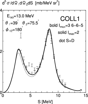
Figure 9: Breakup differential cross sections for the collinear (COLL) configurations. The experimental data are taken from Ref. Gr96 ($pd$ and $nd$) for 10.5 MeV and Refs. Se96,St89 ($nd$) for 13 MeV.

Figure 10: The same as Fig. 9, but for other geometrical configurations and energies. The experimental data are taken from Refs. St89 ($nd$) for 13 MeV, Pa96 ($pd$) for 19 MeV, and Al94 ($pd$) for 65 MeV.

3.8 Non-standard configurations

The comparison with the experimental data for the non-standard configurations is shown in Figs. 11 and 12. Here we find big deviation from the experimental data in some cases, again a common feature with the meson-exchange predictions. These are the NS2 $nd$ scattering of 13 MeV, and the $pd$ scattering of 22.7 MeV and 65 MeV. A large number of figures, NS1 - NS9, for 13 MeV are very similar to the predictions by the Paris potential in Ref. St89. The huge final state interaction peaks in NS4, NS7 and NS8 are very similar to the results by the Malfliet-Tjon potential. In 22.7 MeV and 65 MeV cases, the calculated results are completely off the experimental data.

Figure 11: Breakup differential cross sections for the non-standard (NS) configurations. The experimental data are taken from Ref. St89 ($nd$).

Figure 12: The same as Fig. 11, but for other geometrical configurations and energies. The experimental data are taken from Refs. St89 ($nd$) for 13 MeV, Za94 ($pd$) for 22.7 MeV, and PREP ($pd$) for 65 MeV.

4 Summary

In this and previous papers,[10, 15, 11] we have applied the quark-model (QM) baryon-baryon interaction fss2 to the neutron-deuteron ($nd$) scattering in the Faddeev formalism for composite particles. The main motivation is to investigate the nonlocal effect of the short-range $NN$ interaction in a realistic model, reproducing all the two-nucleon properties and yet based on the naive three-quark structure of the nucleons. The calculations are carried out by the 15-point Gaussian nonlocal potential constructed from fss2, which is accurate enough to reproduce the converged triton binding energy of fss2 with the accuracy of 15 keV and the $NN$ phase shift parameters with the difference of less than $0.1^{\circ}$.[15, 33] The potential keeps all the nonlocal effects of the original fss2, including the energy-dependent term of the QM resonating-group method (RGM). This energy dependence is eliminated by the standard off-shell transformation utilizing the square root of the normalization kernel for two three-quark clusters. It is extremely important to deal with this energy dependence properly, since an extra nonlocal kernel from this procedure is crucial to reproduce all the elastic scattering observables below $E_{n}\leq 65$ MeV.[10, 11]

In this paper, we have studied the neutron-induced deuteron breakup differential cross sections for the incident energies $E_{n}\leq 65$ MeV, and compared them with available experimental data and the predictions by meson-exchange potentials. We have found that our calculations reproduce almost all the results for the breakup differential cross sections predicted by the meson-exchange potentials, including the disagreement with the experiment. This feature is probably related with the structure of the direct breakup amplitudes in Eqs. (18) and (19). First, they are constrained by the elastic scattering amplitudes, $f^{J}_{(\ell^{\prime}S^{\prime}_{c})(\ell S_{c})}$, in the initial stage. In the final stage of reactions, only the half-off shell two-nucleon $t$-matrix appears owing to the energy conservation for outgoing nucleons. The effect of the completely off-shell $t$-matrix therefore appears only at the stage of solving the basic AGS equations for $\widetilde{Q}^{(\ell^{\prime}S^{\prime}_{c})J}_{i\mu\gamma}$, for which the present investigations imply that the difference between our QM $NN$ interaction and the meson-exchange potentials is rather minor. On the whole, the agreement with the experimental data is fair, but there exist some discrepancies in certain particular kinematical configurations, which are commonly found both for our predictions and for meson-exchange predictions. In particular, the space star anomaly of 13 MeV $nd$ scattering is not improved even in our model. There are severe disagreement of breakup differential cross sections in some of the non-standard configurations. In our model, some overestimations of cross sections are found at the energy $E_{n}=65$ MeV. Since these large disagreements can be resolved neither with the Coulomb effect nor by the introduction of the $3N$ force, systematic studies from more basic viewpoints for the $NN$ interaction are still needed both experimentally and theoretically.

In spite of the apparent disagreement between the theory and the experiment in some of the breakup differential cross sections, our QM baryon-baryon interaction fss2 was very successful to reproduce almost all other experimental data of the three-nucleon system without reinforcing it with the three-body force. These include: 1) a nearly correct binding energy of the triton,[13] 2) reproduction of the doublet and quartet $S$-wave scattering lengths, ${}^{2}a$ and ${}^{4}a$,[15] 3) not too small differential cross sections of the $nd$ elastic scattering up to $E_{n}\sim 65$ MeV at the diffraction minimum points,[10] 4) the improved maximum height of the nucleon analyzing power $A_{y}(\theta)$ in the low-energy region $E_{n}\leq 25$ MeV, although not sufficient,[11] and 5) the breakup differential cross sections with many kinematical configurations, discussed in this paper. Many of these improvements are related to the sufficiently attractive $nd$ interaction in the ${}^{2}S$ channel, in which the strong distortion effect of the deuteron is very sensitive to the treatment of the short-range repulsion of the $NN$ interaction. In our QM $NN$ interaction, this part is described by the quark exchange kernel of the color-magnetic term of the quark-quark interaction. In the strangeness sector involving the $\Lambda N$ and $\Sigma N$ interactions, the effect of the Pauli repulsion on the quark level appears in some baryon channels. It is therefore interesting to study $\Sigma^{\pm}$-deuteron scattering in the present framework, to find the repulsive effect directly related to the quark degree of freedom. Such an experiment is planned at the J-PARC facility.[34]

Appendix A Three-nucleon breakup kinematics

In this appendix, we will discuss the $3N$ breakup kinematics used in this paper. We choose the standard set of Jacobi coordinate in the momentum space as $\alpha=3$ and set

$${\boldsymbol{p}}=\frac{1}{2}({\boldsymbol{k}}_{1}-{\boldsymbol{k}}_{2})\ ,\quad{\boldsymbol{q}}=\frac{1}{3}(2{\boldsymbol{k}}_{3}-{\boldsymbol{k}}_{1}-{\boldsymbol{k}}_{2})\ ,\quad{\boldsymbol{K}}={\boldsymbol{k}}_{1}+{\boldsymbol{k}}_{2}+{\boldsymbol{k}}_{3}\ ,$$ (23)

with ${\boldsymbol{k}}_{\alpha}$ being the momentum coordinate of the particle $\alpha$ in the lab system. We also choose the $z$-axis as the direction of the incident particle and assume that the magnitude of the incident momentum is $q_{0}$ in the cm system. This implies that the incident momentum is always ${\boldsymbol{q}}_{\rm cm}=q_{0}{\boldsymbol{e}}_{z}$ and the incident energy is $E_{\rm cm}=(3\hbar^{2}/4M){q_{0}}^{2}$, either the nucleon or the deuteron is the incident particle. Here, ${\boldsymbol{e}}_{z}$ is the unit vector of the $z$-axis. In the lab system, the incident momentum ${\boldsymbol{k}}_{\rm lab}$ and the energy $E_{\rm lab}$ are given by

$$\left\{\begin{array}[]{l}{\boldsymbol{k}}_{\rm lab}=\frac{3}{2}q_{0}{\boldsymbol{e}}_{z}\ ,\\[5.69054pt] E_{\rm lab}=\frac{\hbar^{2}}{2M}{{\boldsymbol{k}}_{\rm lab}}^{2}=\frac{9\hbar^{2}}{8M}{q_{0}}^{2}=\frac{3}{2}E_{\rm cm}\\ \end{array}\right.\quad\hbox{for}\quad\hbox{nucleon-incident}\ ,$$ (26)

$$\left\{\begin{array}[]{l}{\boldsymbol{k}}_{\rm lab}=3q_{0}{\boldsymbol{e}}_{z}\ ,\\[5.69054pt] E_{\rm lab}=\frac{\hbar^{2}}{4M}{{\boldsymbol{k}}_{\rm lab}}^{2}=\frac{9\hbar^{2}}{4M}{q_{0}}^{2}=3E_{\rm cm}\end{array}\right.\quad\hbox{for}\quad\hbox{deuteron-incident}\ .$$ (29)

In the following, all quantities in the initial state are expressed by $k_{\rm lab}=|{\boldsymbol{k}}_{\rm lab}|$ and $E_{\rm cm}$, which are determined solely by $q_{0}$.

In the experimental setup to detect two particles 1 and 2, the three-particle breakup configurations are uniquely specified with two polar angles $\theta_{1}$, $\theta_{2}$, and a difference of azimuthal angles $\phi_{12}=\phi_{1}-\phi_{2}$, in addition to the energy $S$ discussed below. These angles are defined through $\cos\,\theta_{\alpha}=(\widehat{{\boldsymbol{k}}}_{\alpha}\cdot{\boldsymbol{e}}_{z})$ and ${\rm tan}\,\phi_{\alpha}=(k_{\alpha y}/k_{\alpha x})$. We will choose the $x$-axis such that $\phi_{1}=\pi$. [16] If $k_{1}=|{\boldsymbol{k}}_{1}|$ and $k_{2}=|{\boldsymbol{k}}_{2}|$ are determined from $S$, $k_{3}=|{\boldsymbol{k}}_{3}|$ and all other angles in the lab system are calculated from

$$k_{3}=\left[(k_{\rm lab}-k_{1}\cos\,\theta_{1}-k_{2}\cos\,\theta_{2})^{2}+(k_{1}\sin\,\theta_{1})^{2}+(k_{2}\sin\,\theta_{2})^{2}\right.$$

$$\left.\qquad+2k_{1}k_{2}\,\sin\,\theta_{1}\,\sin\,\theta_{2}~{}\cos\,\phi_{12}\right]^{1/2}\ ,$$

$$\cos\,\theta_{3}=\frac{1}{k_{3}}\left(k_{\rm lab}-k_{1}\cos\,\theta_{1}-k_{2}\cos\,\theta_{2}\right)\ ,$$

$$\sin\,\theta_{3}=\frac{1}{k_{3}}\left[(k_{1}\sin\,\theta_{1})^{2}+(k_{2}\sin\,\theta_{2})^{2}+2k_{1}k_{2}\,\sin\,\theta_{1}\,\sin\,\theta_{2}~{}\cos\,\phi_{12}\right]^{1/2}\ ,$$

$$\cos\,\phi_{3}=\frac{1}{k_{3}\sin\,\theta_{3}}\left(k_{1}\sin\,\theta_{1}+k_{2}\,\sin\,\theta_{2}\,\cos\,\phi_{12}\right)\ ,$$

$$\sin\,\phi_{3}=-\frac{1}{k_{3}\sin\,\theta_{3}}k_{2}\,\sin\,\theta_{2}\,\sin\,\phi_{12}\ ,$$ (30)

with $\phi_{1}=\pi$ and $\phi_{2}=\pi-\phi_{12}$. Once all the momentum vectors in the lab system are determined, the momentum vectors in the cm system are easily determined from the relationship, ${\boldsymbol{p}}=(1/2)({\boldsymbol{k}}_{1}-{\boldsymbol{k}}_{2})$ and ${\boldsymbol{q}}=(2/3){\boldsymbol{k}}_{\rm lab}-{\boldsymbol{k}}_{1}-{\boldsymbol{k}}_{2}$ for $\alpha=3$, and their cyclic permutations of (123). The basic magnitude of $q=|{\boldsymbol{q}}|$ is obtained from $k_{3}$ in Eq. (30) by a simple replacement of $k_{\rm lab}$ with $(2/3)k_{\rm lab}$:

$$q = \left[((2/3)k_{\rm lab}-k_{1}\cos\,\theta_{1}-k_{2}\cos\,\theta_{2})^{2}+(k_{1}\sin\,\theta_{1})^{2}+(k_{2}\sin\,\theta_{2})^{2}\right.$$ (31)

$$\left.+2k_{1}k_{2}\,\sin\,\theta_{1}\,\sin\,\theta_{2}~{}\cos\,\phi_{12}\right]^{1/2}\ .$$

The two-nucleon momentum $p=|{\boldsymbol{p}}|$ is determined from the energy conservation in the cm system:

$$E=E_{\rm cm}+\varepsilon_{d}=\frac{\hbar^{2}}{M}\left(p^{2}+\frac{3}{4}q^{2}\right)\ ,$$ (32)

where $\varepsilon_{d}=-(3\hbar^{2}/4M){\kappa_{d}}^{2}$ is the deuteron energy. It is convenient to use the threshold momentum $q_{M}=\sqrt{{q_{0}}^{2}-{\kappa_{d}}^{2}}$ for the deuteron breakup, by which we find

$$p=\sqrt{\frac{3}{4}({q_{M}}^{2}-q^{2})}\equiv p_{0}\ .$$ (33)

The angles of $\widehat{{\boldsymbol{p}}}$ and $\widehat{{\boldsymbol{q}}}$ are obtained from

$$\cos\,\theta_{p}=\frac{1}{2p}\left(k_{1}\cos\,\theta_{1}-k_{2}\cos\,\theta_{2}\right)\ ,$$

$$\cos\,\phi_{p}=\frac{1}{2p\sin\,\theta_{p}}\left(k_{1}\sin\,\theta_{1}\,\cos\,\phi_{1}-k_{2}\sin\,\theta_{2}\,\cos\,\phi_{2}\right)\ ,$$

$$\sin\,\phi_{p}=\frac{1}{2p\sin\,\theta_{p}}\left(k_{1}\sin\,\theta_{1}\,\sin\,\phi_{1}-k_{2}\sin\,\theta_{2}\,\sin\,\phi_{2}\right)\ ,$$

$$\cos\,\theta_{q}=\frac{1}{q}\left(\frac{2}{3}k_{\rm lab}-k_{1}\cos\,\theta_{1}-k_{2}\cos\,\theta_{2}\right)\ ,$$

$$\cos\,\phi_{q}=-\frac{1}{q\sin\,\theta_{q}}\left(k_{1}\sin\,\theta_{1}\,\cos\,\phi_{1}+k_{2}\sin\,\theta_{2}\,\cos\,\phi_{2}\right)\ ,$$

$$\sin\,\phi_{q}=-\frac{1}{q\sin\,\theta_{q}}\left(k_{1}\sin\,\theta_{1}\,\sin\,\phi_{1}+k_{2}\sin\,\theta_{2}\,\sin\,\phi_{2}\right)\ .$$ (34)

In order to determine $k_{1}$ and $k_{2}$ from $S$, we start from the energy conservation in the lab system:

$$E_{\rm lab}+\varepsilon_{d}=\frac{\hbar^{2}}{2M}\left({{\boldsymbol{k}}_{1}}^{2}+{{\boldsymbol{k}}_{2}}^{2}+{{\boldsymbol{k}}_{3}}^{2}\right)\ .$$ (35)

We rewrite this as

$${k_{1}}^{2}+{k_{2}}^{2}+k_{1}k_{2}\,\cos\,\theta_{12}-k_{\rm lab}(k_{1}\,\cos\,\theta_{1}+k_{2}\,\cos\,\theta_{2})+\Delta=0\ ,$$ (36)

where $\cos\,\theta_{12}=(\widehat{{\boldsymbol{k}}}_{1}\cdot\widehat{{\boldsymbol{k}}}_{2})$, and we have defined

$$\Delta\equiv-\frac{M}{\hbar^{2}}\left(E_{\rm lab}+\varepsilon_{d}\right)+\frac{1}{2}{k_{\rm lab}}^{2}=\left\{\begin{array}[]{l}\frac{3}{4}{\kappa_{d}}^{2}\\[5.69054pt] \frac{1}{4}{k_{\rm lab}}^{2}+\frac{3}{4}{\kappa_{d}}^{2}\\ \end{array}\right.\quad\hbox{for}\quad\left\{\begin{array}[]{l}\hbox{nucleon-incident}\\[5.69054pt] \hbox{deuteron-incident}\\ \end{array}\right.\ .$$ (41)

(42)

We rotate $k_{1}$-$k_{2}$ plane by $45^{\circ}$,[1] and parametrize the ellipse with an angle $\theta$. In this process, it is convenient to express $\theta_{12}$ by $\theta_{0}$, which is defined by

$$\theta_{0}=\frac{1}{2}\hbox{Arccos}\left(\frac{1}{2}\cos\,\theta_{12}\right)\ .$$ (43)

Here, Arccos implies the principal value between 0 and $\pi$. Note that $\theta_{0}$ changes from $\pi/6$ to $\pi/3$ for the change of $\theta_{12}$ from 0 to $\pi$. If we use this $\theta_{0}$, the solution of Eq. (36) is parametrized as

$$k_{1}=\frac{k_{\rm lab}}{2\sqrt{2}}\,\frac{A}{\sin\,2\theta_{0}}\,{\cal C}(\theta-\theta_{0})\ \ ,\qquad k_{2}=\frac{k_{\rm lab}}{2\sqrt{2}}\,\frac{A}{\sin\,2\theta_{0}}\,{\cal S}(\theta-\theta_{0})\ ,$$ (44)

with

$${\cal C}(\theta)=\cos\,\theta+{\cal C}_{0}\ \ ,\qquad{\cal S}(\theta)=\sin\,(\theta+2\theta_{0}-\pi/2)+{\cal S}_{0}\ ,$$ (45)

and

$$\ {\cal C}_{0}=\frac{\sqrt{2}}{A}\,\frac{\cos\,\theta_{1}-\cos\,2\theta_{0}\,\cos\,\theta_{2}}{\sin\,2\theta_{0}}\ ,\quad{\cal S}_{0}=\frac{\sqrt{2}}{A}\,\frac{\cos\,\theta_{2}-\cos\,2\theta_{0}\,\cos\,\theta_{1}}{\sin\,2\theta_{0}}\ .$$ (46)

In Eq. (44), we have defined

$$A=\sqrt{2}\left\{\frac{(\cos\,\theta_{1})^{2}+(\cos\,\theta_{2})^{2}-2\cos\,2\theta_{0}\,\cos\,\theta_{1}\,\cos\,\theta_{2}}{(\sin\,2\theta_{0})^{2}}-\frac{4\Delta}{{k_{\rm lab}}^{2}}\right\}^{\frac{1}{2}}\ .$$ (47)

We measure the arc length $S$ in the $E_{1}$-$E_{2}$ plane counterclockwise, starting from a certain starting point $\theta_{\rm st}$. The expression $S(\theta)$ is obtained by integrating $d\,S=\sqrt{(d\,E_{1})^{2}+(d\,E_{2})^{2}}$:

$$S(\theta)=\frac{\hbar^{2}{k_{\rm lab}}^{2}}{2M}\left(\frac{A}{2\,\sin\,2\theta_{0}}\right)^{2}\int^{\theta}_{\theta_{\rm st}}d\,\theta~{}f(\theta-\theta_{0})\ ,$$ (48)

with

$$f(\theta)=\sqrt{\left({\cal C}(\theta)\,\sin\,\theta\right)^{2}+\left({\cal S}(\theta)\,\cos\,(\theta+2\theta_{0}-\pi/2)\right)^{2}}\ .$$ (49)

Note that $S(\theta)$ is a monotonically increasing function of $\theta$, satisfying $S(\theta_{\rm st})=0$ and $S(\theta+2\pi)=S(2\pi)+S(\theta)$.

For the practical calculation, we first discretize the integral region of Eq. (48) into small intervals by

$$\theta_{\mu}=\theta_{\rm st}+\mu\frac{2\pi}{N}\ ,$$ (50)

with $\mu=1$ - $N$. The number of discretization points $N$ is typically $N=50$. We use third order spline interpolation for $\theta$,

$$f(\theta-\theta_{0})=\sum^{N}_{\nu=1}S^{(\kappa)}_{\nu}(\theta)\,f(\theta_{\nu}-\theta_{0})\ ,$$ (51)

with

$$S^{(\kappa)}_{\nu}(\theta)=\sum^{3}_{m=0}\alpha^{\kappa(m)}_{\nu}(\theta-\theta_{\kappa})^{m}\qquad\hbox{for}\qquad\theta\in[\theta_{\kappa-1},\theta_{\kappa}]\ .$$ (52)

If we integrate Eq. (48) over $\theta$ from $\theta_{\rm st}$ to $\theta_{\mu}$ by using Eqs. (51) and (52), we can carry out the $\theta$-integral analytically and obtain

$$S_{\mu} = S(\theta_{\mu})=\frac{\hbar^{2}{k_{\rm lab}}^{2}}{2M}\left(\frac{A}{2\,\sin\,2\theta_{0}}\right)^{2}$$ (53)

$$\times\sum^{3}_{m=0}(-1)^{m+1}\frac{1}{m+1}\left(\frac{2\pi}{N}\right)^{m+1}\sum^{N}_{\nu=1}\sum^{\mu}_{\kappa=1}\alpha^{\kappa(m)}_{\nu}f(\theta_{\nu}-\theta_{0})\ .$$

To obtain the angle $\theta$ from the arc length $S$, we again use the spline interpolation technique,

$$\theta(S)=\sum^{N}_{\mu=1}S_{\mu}(S)\,\theta(S_{\mu})\ .$$ (54)

Here, $S_{\mu}(S)$ is the third order spline function for the mesh points $\{S_{\mu}\}=[S_{0},S_{1},S_{2},$ $\cdots,S_{N}]$ with $S_{0}=0$. From Eq. (54) with $\theta(S_{\mu})=\theta_{\mu}$, we obtain

$$\theta(S)=\theta_{\rm st}+\frac{2\pi}{N}\sum^{N}_{\mu=1}\mu\,S_{\mu}(S)\ ,$$ (55)

where Eq. (50) and $\sum^{N}_{\mu=1}S_{\mu}(S)=1$ are used. We therefore only need to calculate the sum in Eq. (53) and prepare the coefficients of the spline interpolation for the mesh points $\{S_{\mu}\}$.

The starting angle $\theta$ is selected as follows. Let us first consider the nucleon-incident reaction. In this case, it is convenient to define the angle $\theta^{(-)}$ through [1]

$$\cos\,\theta^{(-)}=\frac{2\sqrt{\Delta}}{k_{\rm lab}}=\frac{2}{\sqrt{3}}\,\frac{\kappa_{d}}{q_{0}}\ .$$ (56)

If we assume $k_{2}$=0 in Eq. (36), we find that there are two non-negative solutions

$$k^{(\pm)}_{1}=\frac{k_{\rm lab}}{2}\left[\cos\,\theta_{1}\pm\sqrt{(\cos\,\theta_{1})^{2}-(\cos\,\theta^{(-)})^{2}}\right]\ ,$$ (57)

only when $\theta_{1}<\theta^{(-)}$. We choose the larger value $k^{(+)}_{1}$ as the starting point to measure $S$. In this case, we can easily find that the corresponding $\theta$ value is given by

$$\theta_{\rm st}=\hbox{Arccos}\,{\cal S}_{0}-\theta_{0}\ ,$$ (58)

where ${\cal S}_{0}$ is given in Eq. (46). When $\theta_{1}>\theta^{(-)}$, we have two cases. In the case of $\theta_{2}\leq\theta^{(-)}$, we choose $k_{1}=0$ and

$$k^{(-)}_{2}=\frac{k_{\rm lab}}{2}\left[\cos\,\theta_{2}-\sqrt{(\cos\,\theta_{2})^{2}-(\cos\,\theta^{(-)})^{2}}\right]\ ,$$ (59)

as the starting point with

$$\theta_{\rm st}=\hbox{Arccos}\,{\cal C}_{0}+\theta_{0}-\pi\ .$$ (60)

In the case of $\theta_{2}>\theta^{(-)}$, the ellipse does not cross over either $k_{1}$ or $k_{2}$ axis. We therefore use the smaller value of $k_{1}=k_{2}$ as the starting point. This condition yields

$$\theta_{\rm st}=\hbox{Arccos}\left(\frac{1}{A}\,\frac{\cos\,\theta_{1}-\cos\,\theta_{2}}{\sqrt{2}\,\sin\,\theta_{0}}\right)+\pi\ ,$$ (61)

and

$$k^{(-)}_{1}=k^{(-)}_{2}=\frac{k_{\rm lab}}{4\,\cos\,\theta_{0}}\left[\frac{\cos\,\theta_{1}+\cos\,\theta_{2}}{2\,\cos\,\theta_{0}}-\sqrt{\left(\frac{\cos\,\theta_{1}+\cos\,\theta_{2}}{2\,\cos\,\theta_{0}}\right)^{2}-\frac{4\Delta}{{k_{\rm lab}}^{2}}}\right]\ .$$

(62)

When the deuteron is an incident particle, there is no crossing point across either the $k_{1}$-axis or the $k_{2}$-axis. We follow the definition of the Correll et al.’s paper [17], that discusses the deuteron incident reaction around the collinear configurations, choosing the collinear point as the starting point to measure $S$. The collinear point $\theta_{c}$ is defined as the configuration with ${\boldsymbol{q}}=(2/3){\boldsymbol{k}}_{\rm lab}-({\boldsymbol{k}}_{1}+{\boldsymbol{k}}_{2})=0$. To find the corresponding $\theta_{\rm st}=\theta_{c}$, we assume $\phi_{12}=\pi$ ($\phi_{1}=\pi$, $\phi_{2}=0$) and the $x$-$z$ plane as the reaction plane, just as the experimental setup. Under this assumption, the magnitude ${\boldsymbol{q}}^{2}$ is expressed as

$${\boldsymbol{q}}^{2}=\left(k_{1}\,\cos\,\theta_{1}+k_{2}\,\cos\,\theta_{2}-\frac{2}{3}k_{\rm lab}\right)^{2}+\left(k_{1}\,\sin\,\theta_{1}-k_{2}\,\sin\,\theta_{2}\right)^{2}\ ,$$ (63)

resulting in the two conditions

$$k_{1}\,\cos\,\theta_{1}+k_{2}\,\cos\,\theta_{2}=\frac{2}{3}k_{\rm lab}\ \ ,\qquad k_{1}\,\sin\,\theta_{1}=k_{2}\,\sin\,\theta_{2}\ .$$ (64)

If $\theta_{1}=\theta_{2}$, we assume $k_{1}=k_{2}$ and find $\theta_{c}=\pi/2$ with

$$k_{1}=k_{2}=\frac{k_{\rm lab}}{4}\left(\frac{\cos\,\theta_{1}}{(\cos\,\theta_{0})^{2}}+\frac{A}{\sqrt{2}\,\cos\,\theta_{0}}\right)\ .$$ (65)

This corresponds to the $k^{(+)}_{1}=k^{(+)}_{2}$ case of Eq. (62) with the opposite sign for the second term. In the general case, the three conditions of Eq. (64) and the energy conservation in Eq. (36) are not always simultaneously satisfied. (Note that we only need two conditions to determine $k_{1}$ and $k_{2}$.) We take the following procedure to determine $\theta_{c}$. Let us use the notation

$$a=\frac{\cos\,\theta_{1}-\cos\,\theta_{2}}{\sqrt{2}\,\sin\,\theta_{0}}\ \ ,\qquad b=\frac{\cos\,\theta_{1}+\cos\,\theta_{2}}{\sqrt{2}\,\cos\,\theta_{0}}\ ,$$ (66)

to simplify the expressions. We have $a^{2}+b^{2}=A^{2}+(8\Delta/{k_{\rm lab}}^{2})$ and define a new angle $\alpha$ by

$$\cos\,\alpha=\frac{a}{\sqrt{a^{2}+b^{2}}}\ \ ,\qquad\sin\,\alpha=\frac{b}{\sqrt{a^{2}+b^{2}}}\ .$$ (67)

We consider, $I(\theta)=k_{1}\cos\,\theta_{1}+k_{2}\cos\,\theta_{2}$, as a function of $\theta$, by using Eq. (44) and others. We find

$$\ I(\theta) = k_{1}\cos\,\theta_{1}+k_{2}\cos\,\theta_{2}=\frac{1}{4}k_{\rm lab}\sqrt{a^{2}+b^{2}}\left[A\,\cos\,(\theta-\alpha)+\sqrt{a^{2}+b^{2}}\right]\ .$$ (68)

The crossing point with $I(\theta)=(2/3)k_{\rm lab}$ is found only when the condition

$$\frac{1}{A}\left|\frac{8}{3}\frac{1}{\sqrt{a^{2}+b^{2}}}-\sqrt{a^{2}+b^{2}}\right|\leq 1\ ,$$ (69)

is satisfied. The solution $\theta=\theta_{c}$ is found as

$$\theta_{c}=\alpha\pm{\rm Arccos}\,\frac{1}{A}\left[\frac{8}{3}\frac{1}{\sqrt{a^{2}+b^{2}}}-\sqrt{a^{2}+b^{2}}\right]\ ,$$ (70)

and a unique point is determined when the equality is satisfied in Eq. (69). Next, we examine the condition, $k_{1}\,\sin\,\theta_{1}=k_{2}\,\sin\,\theta_{2}$, is satisfied or not for the two solutions of Eq. (70). The one satisfying this condition is the collinear point with ${\boldsymbol{q}}=0$ from Eq. (63). If both solutions satisfy the condition, we choose the smaller one for $\theta_{c}$. If neither of the solution satisfies the condition, there is no exact collinear point. In this case, we minimize Eq. (63) with respect to $\theta$ in the interval bounded by the two solutions of Eq. (70).

Appendix B Isospin factors for the breakup amplitudes

In this appendix, we extend the definition of the spin factors

$$\langle\widetilde{\Gamma}_{\sigma}|(P^{\sigma}_{(123)})^{\alpha}|\Gamma_{\sigma}\rangle=\delta_{\widetilde{S},S}\,\delta_{\widetilde{S}_{z},S_{z}}\left\{\begin{array}[]{c}(-1)^{1+s}X^{S}_{\widetilde{s},s}\\[5.69054pt] (-1)^{1+\widetilde{s}}X^{S}_{\widetilde{s},s}\\[5.69054pt] \delta_{\widetilde{s},s}\\ \end{array}\right.\quad\hbox{for}\quad\alpha=\left\{\begin{array}[]{c}1\\[5.69054pt] 2\\[5.69054pt] 3\\ \end{array}\right.\ ,$$ (77)

to the isospin factors and calculate the matrix elements $\langle\widetilde{\Gamma_{\tau}}|{\cal O}^{\alpha\beta}_{\tau}|\Gamma_{\tau}\rangle$ in Eq. (13). The most convenient definition of the isospin factors is probably

$$\langle\widetilde{\Gamma}_{\tau}|{\cal O}^{\alpha\beta}_{\tau}|\Gamma_{\tau}\rangle=\langle(\widetilde{t}{\scriptstyle\frac{1}{2}}){\scriptstyle\frac{1}{2}}T_{z}|(P^{\tau}_{(123)})^{3-\alpha}{\cal O}_{\tau}(P^{\tau}_{(123)})^{\beta}|(t{\scriptstyle\frac{1}{2}}){\scriptstyle\frac{1}{2}}T_{z}\rangle$$

$$=\left\{\begin{array}[]{c}(-1)^{1+t}X^{\tau(\alpha\beta)}_{\widetilde{t},t}\\[5.69054pt] (-1)^{1+\widetilde{t}}X^{\tau(\alpha\beta)}_{\widetilde{t},t}\\[5.69054pt] X^{\tau(\alpha\alpha)}_{\widetilde{t},t}\\ \end{array}\right.\quad\hbox{for}\quad\beta-\alpha=\left\{\begin{array}[]{c}1\\[5.69054pt] 2\\[5.69054pt] 3\\ \end{array}\right.\quad\hbox{in~{}(mod~{}3)}\ ,$$ (84)

which yields the results in Eq. (14). If we set ${\cal O}_{\tau}=1$, all the factors $X^{\tau(\alpha\beta)}_{\widetilde{t},t}$ in Eq. (84) are reduced to $X^{1/2}_{\widetilde{t},t}$ since ${\cal O}^{\alpha\beta}_{\tau}=(P^{\tau}_{(123)})^{\beta-\alpha}$. Here, $X^{1/2}$ is the common matrix with the spin factors given by[15]

$$\left(X^{\scriptstyle\frac{1}{2}}_{s,s^{\prime}}\right)=\left(\begin{array}[]{cc}\frac{1}{2}&-\frac{\sqrt{3}}{2}\\[5.69054pt] -\frac{\sqrt{3}}{2}&-\frac{1}{2}\\ \end{array}\right)\ \ ,\qquad\left(X^{\scriptstyle\frac{3}{2}}_{s,s^{\prime}}\right)=\left(\begin{array}[]{cc}0&0\\ 0&1\\ \end{array}\right)\ .$$ (89)

In Eq. (89), the upper row (the left-most column) corresponds to $s=0$ ($s^{\prime}=0$) and the second row (the right-most column) corresponds to $s=1$ ($s^{\prime}=1$).

In order to calculate $X^{\tau(\alpha\beta)}_{\widetilde{t},t}$, we only need $\langle\widetilde{t}|{\cal O}_{\tau}|t\rangle$ with $|t\rangle=|(t{\scriptstyle\frac{1}{2}}){\scriptstyle\frac{1}{2}}T_{z}\rangle$, since $P^{\tau}_{(123)}$ does not change the total isospin $T=1/2$. Furthermore, ${\cal O}_{\tau}$ in Eq. (10) are expressed by the symmetric isospin operator $t_{z}=(\tau_{z}(1)+\tau_{z}(2))/2$ and the antisymmetric operator $t^{a}_{z}=(\tau_{z}(1)-\tau_{z}(2))/2$ for the two-particle states $\eta_{t}(1,2)$. The former does not change $t=0$ or 1, while the latter flips the isospin value. For $pp$ or $nn$, the non-zero matrix elements are only for $\widetilde{t}=t=1$, but $np$ and $pn$ contains $t^{a}_{z}$. However, we only need to calculate the sum of $np$ and $pn$ contributions. Furthermore, Eq. (5) tells us that $np$ and $pn$ give the same contribution owing to the permutation operator $(1+P)$. We can therefore assume ${\cal O}_{\tau}$ in Eq. (84) as

$${\cal O}^{pp}=\frac{1}{2}t_{z}(1+t_{z})\ ,\quad{\cal O}^{nn}=\frac{1}{2}t_{z}(-1+t_{z})\ ,\quad{\cal O}^{pn}+{\cal O}^{np}=1-t^{2}_{z}\ .$$ (90)

If we decompose $t^{2}_{z}$ into the rank 0, 1, and 2 tensors as $t^{2}_{z}=(1/3){\boldsymbol{t}}^{2}+\sqrt{2/3}[t\,t]^{(2)}_{0}$, we immediately find that the rank 2 tensor does not contribute since the total isospin in our case is $T=1/2$. We can therefore replace $t^{2}_{z}$ in Eq. (90) with $(1/3){\boldsymbol{t}}^{2}$, resulting in

$$\langle\widetilde{t}|{\cal O}^{pp}|t\rangle=\langle\widetilde{t}|{\cal O}^{nn}|t\rangle=\delta_{\widetilde{t},t}\,\delta_{t,1}\frac{2}{3}\ ,$$

$$\langle\widetilde{t}|{\cal O}^{pn}|t\rangle+\langle\widetilde{t}|{\cal O}^{np}|t\rangle=\delta_{\widetilde{t},t}\,\left(\delta_{t,0}+\frac{1}{3}\delta_{t,1}\right)\ .$$ (91)

It is convenient to introduce the isospin projection operators $P_{0}=(1-{\boldsymbol{\tau}}(1)\cdot{\boldsymbol{\tau}}(2))/4$ and $P_{1}=(3+{\boldsymbol{\tau}}(1)\cdot{\boldsymbol{\tau}}(2))/4$, and define

$$X^{\tau(\alpha\beta)}_{\widetilde{t},t}$$

$$=\left\{\begin{array}[]{c}(-1)^{1+t}\langle\widetilde{t}|(P^{\tau}_{(123)})^{3-\alpha}P_{\tau}(P^{\tau}_{(123)})^{\beta}|t\rangle\\[5.69054pt] (-1)^{1+\widetilde{t}}\langle\widetilde{t}|(P^{\tau}_{(123)})^{3-\alpha}P_{\tau}(P^{\tau}_{(123)})^{\beta}|t\rangle\\[5.69054pt] \langle\widetilde{t}|(P^{\tau}_{(123)})^{3-\alpha}P_{\tau}(P^{\tau}_{(123)})^{\alpha}|t\rangle\\ \end{array}\right.\quad\hbox{for}\quad\beta-\alpha=\left\{\begin{array}[]{c}1\\[5.69054pt] 2\\[5.69054pt] 3\\ \end{array}\right.\quad\hbox{in~{}(mod~{}3)}\ ,$$ (98)

(99)

for $\tau=0$ and 1. Since $P_{\tau}$ is expressed as $P_{\tau}=|\tau\rangle\langle\tau|$ in our model space, the matrix elements $\langle\widetilde{t}|(P^{\tau}_{(123)})^{3-\alpha}P_{\tau}(P^{\tau}_{(123)})^{\beta}|t\rangle=\langle\widetilde{t}|(P^{\tau}_{(123)})^{3-\alpha}|\tau\rangle\langle\tau|(P^{\tau}_{(123)})^{\beta}|t\rangle$ can be easily calculated from Eq. (77). The correspondence

$${\cal O}^{pp},~{}{\cal O}^{nn}\sim\frac{2}{3}P_{1}\ ,\quad{\cal O}^{pn}+{\cal O}^{np}\sim P_{0}+\frac{1}{3}P_{1}\ ,$$ (100)

from Eq. (91) yields

$$X^{pp},~{}X^{nn}=\frac{2}{3}X^{1(\alpha\beta)}\ ,\quad X^{pn}+X^{np}=X^{0(\alpha\beta)}+\frac{1}{3}X^{1(\alpha\beta)}\ ,$$ (101)

in the matrix form. Here $X^{\tau(\alpha\beta)}$ with $\tau=0$ and 1 are given by

($\tau=0$ factors)

$$X^{0(11)}=\left(\begin{array}[]{cc}\frac{1}{4}&\frac{\sqrt{3}}{4}\\[5.69054pt] \frac{\sqrt{3}}{4}&\frac{3}{4}\\ \end{array}\right)\ ,\quad X^{0(22)}=\left(\begin{array}[]{cc}\frac{1}{4}&-\frac{\sqrt{3}}{4}\\[5.69054pt] -\frac{\sqrt{3}}{4}&\frac{3}{4}\\ \end{array}\right)\ ,\quad X^{0(33)}=\left(\begin{array}[]{cc}1&0\\ 0&0\\ \end{array}\right)\ ,$$ (108)

$$X^{0(12)}=X^{0(21)}=\left(\begin{array}[]{cc}-\frac{1}{4}&-\frac{\sqrt{3}}{4}\\[5.69054pt] -\frac{\sqrt{3}}{4}&-\frac{3}{4}\\ \end{array}\right)\ ,$$ (111)

$$X^{0(23)}={}^{t}X^{0(32)}=X^{0(13)}={}^{t}X^{0(31)}=\left(\begin{array}[]{cc}\frac{1}{2}&0\\[5.69054pt] -\frac{\sqrt{3}}{2}&0\\ \end{array}\right)\ .$$ (114)

($\tau=1$ factors)

$$X^{1(11)}=\left(\begin{array}[]{cc}\frac{3}{4}&-\frac{\sqrt{3}}{4}\\[5.69054pt] -\frac{\sqrt{3}}{4}&\frac{1}{4}\\ \end{array}\right)\ ,\quad X^{1(22)}=\left(\begin{array}[]{cc}\frac{3}{4}&\frac{\sqrt{3}}{4}\\[5.69054pt] \frac{\sqrt{3}}{4}&\frac{1}{4}\\ \end{array}\right)\ ,\quad X^{1(33)}=\left(\begin{array}[]{cc}0&0\\ 0&1\\ \end{array}\right)\ ,$$ (121)

$$X^{1(12)}=X^{1(21)}=\left(\begin{array}[]{cc}\frac{3}{4}&-\frac{\sqrt{3}}{4}\\[5.69054pt] -\frac{\sqrt{3}}{4}&\frac{1}{4}\\ \end{array}\right)\ ,$$ (124)

$$X^{1(23)}={}^{t}X^{1(32)}=X^{1(13)}={}^{t}X^{1(31)}=\left(\begin{array}[]{cc}0&-\frac{\sqrt{3}}{2}\\[5.69054pt] 0&-\frac{1}{2}\\ \end{array}\right)\ .$$ (127)

References

• [1] W. Glöckle, H. Witała, D. Hüber, H. Kamada and J. Golak, \PRP274,1996,107.
• [2] See for example, H. Kamada, A. Nogga, W. Glöckle, E. Hiyama, M. Kamimura, K. Varga, Y. Suzuki, M. Viviani, A. Kievsky, S. Rosati, J. Carlson, Steven C. Pieper, R. B. Wiringa, P. Navrátil, B. R. Barrett, N. Barnea, W. Leidemann and G. Orlandini, \PRC64,2001,044001, and references therein.
• [3] J. Kuroś-Żołnierczuk, H. Witała, J. Golak, H. Kamada, A. Nogga, R. Skibiński and W. Glöckle, \PRC66,2002,024003.
• [4] J. Kuroś-Żołnierczuk, H. Witała, J. Golak, H. Kamada, A. Nogga, R. Skibiński and W. Glöckle, \PRC66,2002,024004.
• [5] E. Epelbaum, H. Kamada, A. Nogga, H. Witała, W. Glöckle and Ulf-G. Meißner, \PRL86,2001,4787.
• [6] E. Epelbaum, A. Nogga, W. Glöckle, H. Kamada, Ulf-G. Meißner and H. Witała, \PRC66,2002,064001.
• [7] A. Deltuva, A. C. Fonseca and P. U. Sauer, \PRC71,2005,054005.
• [8] A. Deltuva, A. C. Fonseca and P. U. Sauer, \PRC72,2005,054004.
• [9] S. Ishikawa, \PRC80,2009,054002, and private communications.
• [10] Y. Fujiwara and K. Fukukawa, \PTP124,2010,433.
• [11] K. Fukukawa and Y. Fujiwara, Prog. Theor. Phys. 125 (2011), No. 4 (nucl-th1101.2977).
• [12] Y. Fujiwara, Y. Suzuki and C. Nakamoto, \JLProg. Part. Nucl. Phys.,58,2007,439.
• [13] Y. Fujiwara, K. Miyagawa, M. Kohno, Y. Suzuki and H. Nemura, \PRC66,2002,021001(R); Y. Fujiwara, K. Miyagawa, M. Kohno and Y. Suzuki, \PRC70,2004,024001; Y. Fujiwara, Y. Suzuki, M. Kohno and K. Miyagawa, \PRC77,2008,027001.
• [14] K. Fukukawa and Y. Fujiwara, \JLAIP Conf. Proc.,1235,2010,282.
• [15] K. Fukukawa and Y. Fujiwara, arXiv: nucl-th1010.2024, submitted to Prog. Theor. Phys. (2011).
• [16] G. G. Ohlsen, \JLNucl. Inst. Methods,37,1965,240.
• [17] F. D. Correll, R. E. Brown, G. G. Ohlsen, R. A. Hardekopf, N. Jarmie, J. M. Lambert, P. A. Treado, I. Šlaus, P. Schwandt and P. Doleschall, \NPA475,1987,407.
• [18] H. R. Setze, C. R. Howell, W. Tornow, R. T. Braun, W. Glöckle, A. H. Hussein, J. M. Lambert, G. Mertens, C. D. Roper, F. Salinas, I. Šlaus, D. E. González Trotter, B. Vlahović, R. L. Walter and H. Witała, \PLB388,1996,229.
• [19] K. Gebhardt, W. Jäger, C. Jeitner, M. Vitz, E. Finckh, T. N. Frank, Th. Januschke, W. Sandhas and H. Haberzettl, \NPA561,1993,232.
• [20] R. Großmann, G. Nitzsche, H. Patberg, L. Sydow, S. Vohl, H. Paetz gen. Schieck, J. Golak, H. Witała, W. Glöckle and D. Hüber, \NPA603,1996,161.
• [21] G. Rauprich, S. Lema$\hat{\hbox{i}}$tre, P. Nießen, K. R. Nyga, R. Reckenfelderbäumer, L. Sydow, H. Paetz gen. Schieck, H. Witała and W. Glöckle, \NPA535,1991,313.
• [22] H. Patberg, R. Großmann, G. Nitzsche, L. Sydow, S. Vohl, H. Paetz gen. Schieck, J. Golak, H. Witała, W. Glöckle and D. Hüber, \PRC53,1996,1497.
• [23] M. Zadro, M. Bogovac, G. Calvi, M. Lattuada, D. Miljanic, D. Reudic, C. Spitaleri, B. Vlahovic, H. Witała, W. Glöckle, J. Golak and H. Kamada, \JLIl Nuovo Cimento,107A,1994,185.
• [24] M. Allet, K. Bodek, W. Hajdas, J. Lang, R. Müller, S. Navert, O. Naviliat-Cuncic, J. Sromicki, J. Zejma, L. Jarczyk, St. Kistryn, J. Smyrski, A. Strzałkowski, H. Witała, W. Glöckle, J. Golak, D. Hüber and H. Kamada, \JLFew-Body Systems,20,1996,27.
• [25] C. R. Howell, H. R. Setze, W. Tornow, R. T. Braun, W. Glöckle, A. H. Hussein, J. M. Lambert, G. Mertens, C. D. Roper, F. Salinas, I. Šlaus, D. E. González Trotter, B. Vlahović, R. L. Walter and H. Witała, \NPA631,1998,692c.
• [26] J. Strate, K. Geissdörfer, R. Lin, J. Cub, E. Finckh, K. Gebhardt, S. Schindler, H. Witała, W. Glöckle and T. Cornelius, \JLJ. Phys. G: Nucl. Phys.,14,1988,L229.
• [27] J. Strate, K. Geissdörfer, R. Lin, W. Bielmeier, J. Cub, A. Ebneth, E. Finckh, H. Friess, G. Fuchs K. Gebhardt and S. Schindler, \NPA501,1989,51.
• [28] C. Düweke, R. Emmerich, A. Imig, J. Ley, G. Tenckhoff, H. Paetz gen. Schieck, J. Golak, H. Witała, E. Epelbaum, W. Glöckle and A. Nogga, \PRC71,2005,054003.
• [29] M. Stephan, K. Bodek, J. Krug, W. Lübcke, S. Obermanns, H. Rühl, M. Steinke, D. Kamke, H. Witała, Th. Cornelius and W. Glöckle, \PRC39,1989,2133.
• [30] J. Zejma, M. Allet, K. Bodek, J. Lang, R. Müller, S. Navert, O. Naviliat-Cuncic, J. Sromicki, E. Stephan, L. Jarczyk, St. Kistryn, J. Smyrski, A. Strzałkowski, W. Glöckle, J. Golak, D. Hüber, H. Witała and P. A. Schmelzbach, \PRC55,1997,42.
• [31] F. Foroughi, H. Vuillème, P. Chatelain, C. Nussbaum and B. Favier, \JLJ. Phys. G: Nucl. Phys.,11,1985,59.
• [32] M. Allet, K. Bodek, W. Hajdas, J. Lang, R. Müller, O. Naviliat-Cuncic, J. Sromicki, J. Zejma, L. Jarczyk, St. Kistryn, J. Smyrski, A. Strzałkowski, W. Glöckle, J. Golak, H. Witała, B. Dechant, J. Krug and P. A. Schmelzbach, \PRC50,1994,602.
• [33] K. Fukukawa, Y. Fujiwara and Y. Suzuki, \JLMod. Phys. Lett.,24,2009,1035.
• [34] K. Miwa et al., a proposal at J-PARC.