Energy gap in graphene nanoribbons with structured external electric potentials

Abstract

The electronic properties of graphene zig-zag nanoribbons with electrostatic potentials along the edges are investigated. Using the Dirac-fermion approach, we calculate the energy spectrum of an infinitely long nanoribbon of finite width $w$, terminated by Dirichlet boundary conditions in the transverse direction. We show that a structured external potential that acts within the edge regions of the ribbon, can induce a spectral gap and thus switches the nanoribbon from metallic to insulating behavior. The basic mechanism of this effect is the selective influence of the external potentials on the spinorial wavefunctions that are topological in nature and localized along the boundary of the graphene nanoribbon. Within this single particle description, the maximal obtainable energy gap is $E_{\rm max}\propto\pi\hbar v_{\rm F}/w$, i.e., $\approx 0.12$ eV for $w=$15 nm. The stability of the spectral gap against edge disorder and the effect of disorder on the two-terminal conductance is studied numerically within a tight-binding lattice model. We find that the energy gap persists as long as the applied external effective potential is larger than $\simeq 0.55\times W$, where $W$ is a measure of the disorder strength. We argue that there is a transport gap due to localization effects even in the absence of a spectral gap.

I Introduction

The continuing rise of graphene as a new and exceptionally promising material that outperforms conventional metals and semiconductors has initiated an ongoing quest for new physical effects. This has also generated a multitude of exciting proposals for various technical applications, which have recently been summarized in several reviews.Castro Neto et al. (2008); Beenakker (2008); Castro Neto (2010) However, due to single layer graphene’s gap-less energy structure, applications where considerable on-off current ratios are indispensable are limited at present. Proposals for the creation of a lattice anisotropy that would lift the sublattice symmetry,Giovannetti et al. (2007) or for the application of strain fields Gui et al. (2008); Pereira et al. (2009) that also could open an energy gap have yet to be realized. At present, bilayer graphene or certain graphene arm-chair nanoribbons have to be utilized instead, if an energy gap is needed. In the latter case, narrow ribbons of special widths have to be fabricated so that, due to quantum confinement, an energy gap or at least a transport gap in disordered ribbons is formed. For ribbon widths below 30 nm, the spectral gap is larger than $kT$ at room temperature.Han et al. (2007); Lin et al. (2008) Recently, the effect of a transversal electric field on arm-chair ribbons has also been studied theoretically.Novikov (2007)

Within simple non-interacting particle descriptions, graphene zig-zag ribbons are metallic and the opening of a spectral gap is impeded by electronic edge states Fujita et al. (1996); Nakada et al. (1996); Wakabayashi et al. (2009) appearing in an energy range where for broad two-dimensional graphene sheets valence and conduction bands touch. These edge states are sensitive to an Aharonov-Bohm flux and robust against edge reconstructions.Sasaki et al. (2006, 2008) For interacting electrons, it was shown Son et al. (2006a) that zig-zag ribbons always have a gap due to edge magnetization and that a homogeneous external electric field applied across the ribbon causes a half-metallic state.Son et al. (2006b) By employing the ab initio pseudopotential density functional method,Solér et al. (2002) the authors of Ref. Son et al., 2006b studied the spin-resolved electronic structure of zig-zag graphene nanoribbons and the possibility of spin-polarized currents. The influence of electron transfer between the two edges on the half-metallicity of the nanoribbon subjected to the electric field was also investigated.Kan et al. (2007) Recently, a gapped magnetic ground state has been suggested to be due to an antiferromagnetic interedge superexchange.Jung et al. (2009)

These advanced theories are extremely interesting for clean graphene zig-zag nanoribbons. However, there is still no conclusive direct experimental observation proving the existence of an one-dimensional magnetic state. The latter may well be spoiled in reality by edge disorder or adsorbent atoms.Kunstmann et al. (2011) Therefore, we try to clarify in this paper whether one can obtain a spectral gap already within a single particle description. In order to substantiate the relevance of such a basic model for real graphene zig-zag nanoribbons, we investigate the influence of edge disorder on both the spectral properties and the two-terminal electronic transport. In our work, we first investigate a very simple spinless continuum model that can be treated analytically and then we employ a tight-binding lattice model including edge disorder effects, which we solve numerically.

Based on the Dirac equation for two-dimensional electrons with Dirichlet boundary conditions imposed in the transverse direction, we study in section II the influence of an effective potential acting within narrow strips along the edge regions of the graphene zig-zag nanoribbon. This set-up, as sketched in Fig. 1, can be studied experimentally in a three-dimensional device by applying voltages between the back-gate of a graphene zig-zag ribbon and two top gates, one at the right and the other one at the left edge, respectively. The results are given in section III. For a perfectly antisymmetric electric potential (left side $V$ and right side $-V$, see Fig. 1), we find a symmetric spectral gap at the Dirac point, which increases linearly with the applied voltage $V$. Increasing the potential further, the gap reaches a maximum value of $\sim\pi/w$, where $w$ is the width of the ribbon, and finally closes again for even larger $V$. The splitting of the edge state energies, however, still continues to rise with $V$.

In order to check how these results are influenced by disorder, we study numerically a tight-binding lattice model in section IV, calculate the two-terminal conductance, and investigate the influence of edge disorder on both the spectral and the transport gap. The former survives for $V$ being larger than $0.55\times W$, where $W^{2}/3$ is the 2nd moment of the distribution $P(\epsilon)=1/(2W)\Theta(W-|\epsilon|)$ that defines the disorder potentials assumed along the ribbon edges. A transport gap, however, is still observable even for very strong disorder when the spectral gap is absent.

II Model and solution

We study a zig-zag nanoribbon of graphene, infinitely extended in $x$-direction and with finite width $w$ in $y$-direction (see Fig. 1) using the Dirac-type equation approximation. This Dirac-fermion approach usually describes correctly the low-lying states around the neutrality point in graphene.Ando et al. (1998); Katsnelson et al. (2006); Gusynin and Sharapov (2005); Ando (2007); Beenakker (2008) There are two inequivalent (Dirac) points at $\mathbf{k}=\pm\mathbf{K}$ (valleys) in the band structure where valence band and conduction band touch. The wave function for wave vectors near $\mathbf{K}$ is written as $(\xi(a,\mathbf{x}),\xi(b,\mathbf{x}))$, where $a$ and $b$ denote the two sublattices of the graphene structure. Correspondingly, $(\eta(a,\mathbf{x}),\eta(b,\mathbf{x}))$ is the wave function in the other valley. Since the Hamiltonian does not mix the valleys near $\mathbf{K}$ and $-\mathbf{K}$, the Dirac equation separates and reads for the first valley (in the other valley, we have a corresponding equation with $i\partial_{x}\to-i\partial_{x}$)

$$\left(\begin{array}[]{cc}E-V(y)&\hbar v_{\mathrm{F}}(i\partial_{x}-\partial_{y})\\ \hbar v_{\mathrm{F}}(i\partial_{x}+\partial_{y})&E-V(y)\end{array}\right)\left(\begin{array}[]{cc}\xi(a,\mathbf{x})\\ \xi(b,\mathbf{x})\end{array}\right)=0.$$ (1)

Here, $v_{\mathrm{F}}\simeq 10^{6}$ m/s is the Fermi velocity, $E$ the energy, and $V$ the electrostatic potential depending only on the $y$-coordinate. In what follows, we set $\hbar v_{\mathrm{F}}=1$ but recover the units when showing our results in the figures. In the corresponding lattice model, the boundaries at $y=0$ and $y=w$ are considered to be of zig-zag type. Then, in a description in terms of the Dirac model, we have periodic boundary conditions in the $x$-direction and Dirichlet boundary conditions in the $y$-direction such that $\xi(a,x,y=0)=0$ and $\xi(b,x,y=w)=0$.Brey and Fertig (2006)

Figure 1: Cross section of a graphene zig-zag nanoribbon of width $w$ (dashed line) showing the effective potential $V(y)$ created by external voltages applied between the back-gate and two top-gates. The top-gates extend in the $x$ direction along the left and the right edge having widths $y_{L}$ and $w-y_{R}$, respectively.

In order to have a simple model that can be treated analytically, we consider a piecewise constant electrostatic potential $V(y)=V$ for $0\leq y\leq y_{L}$, $V(y)=0$ for $y_{L}<y<y_{R}$, and $V(y)=-V$ for $y_{R}\leq y\leq w$ (see Fig. 1). At the points $y_{L}$ and $y_{R}$ the potential jumps, giving rise to a singular electric field only at $y_{L}$ and $y_{R}$ within the two-dimensional graphene sheet pointing into the $y$ direction and being zero otherwise. $\pm V$ denotes the strength of the potential of the respective potential steps. This special choice leads to a symmetric energy gap around the Dirac points at $E=0$ if $y_{L}=w-y_{R}$.

Due to the periodic boundary conditions in the $x$-direction, it is convenient to take the Fourier-transforms $\xi(a,\mathbf{x})=e^{iqx}\xi(a,q,y)$, $\xi(b,\mathbf{x})=e^{iqx}\xi(b,q,y)$ and make the following ansatz for the wave function $\xi(a,q,y)$ in the three regions of $y$

$$\xi(a,q,y)=\left\{\begin{array}[]{l}L_{+}e^{ik_{L}y}+L_{-}e^{-ik_{L}y},\hfill y\leq y_{L}\\ M_{+}e^{ik_{M}y}+M_{-}e^{-ik_{M}y},\hfill y_{L}<y<y_{R}\\ R_{+}e^{ik_{R}(y-w)}+R_{-}e^{-ik_{R}(y-w)},\hfill y_{R}\leq y\end{array}\right.$$ (2)

where $k_{L,R}$ and $k_{M}$ are given by

$$k_{L,R}=\sqrt{(E\mp V)^{2}-q^{2}},\quad k_{M}=\sqrt{E^{2}-q^{2}}.$$ (3)

The roots are defined to be positive if $E$ is large and the usual analytic continuation is taken otherwise. $\xi(b,q,y)$ is then obtained from the Dirac equation as

$$\xi(b,q,y)=\left\{\begin{array}[]{lll}q^{*}_{L}L_{+}e^{ik_{L}y}+q_{L}L_{-}e^{-ik_{L}y},\hfill y\leq y_{L}\\ q^{*}_{M}M_{+}e^{ik_{M}y}+q_{M}M_{-}e^{-ik_{M}y},\hfill y_{L}<y<y_{R}\\ q^{*}_{R}R_{+}e^{ik_{R}(y-w)}+q_{R}R_{-}e^{-ik_{R}(y-w)},\hfill y_{R}\leq y\end{array}\right.$$ (4)

with

$$q_{L,R}=\frac{q+ik_{L,R}}{E\mp V},\quad q_{M}=\frac{q+ik_{M}}{E}.$$ (5)

Here, $q_{M}^{*}$ is given by $q_{M}|_{k_{M}\to-k_{M}}$ even for imaginary $k_{M}$ and we have $q_{M}^{*}q_{M}=1$. The same applies to $q_{L,R}$.

The six amplitudes $L_{\pm}$, $M_{\pm}$, and $R_{\pm}$ follow from the normalization, from the boundary conditions

$$\xi(a,q,0) = L_{+}+L_{-}=0$$

$$\xi(b,q,w) = q_{R}^{*}R_{+}+q_{R}R_{-}=0,$$ (6)

and from the matching conditions for $\xi(a,q,y)$ and $\xi(b,q,y)$ at $y_{L,R}$

$$e_{L}L_{+}+e_{L}^{*}L_{-} = M_{+}^{\prime}+M_{-}^{\prime}$$

$$e_{M}M_{+}^{\prime}+e_{M}^{*}M_{-}^{\prime} = e_{R}^{*}R_{+}+e_{R}R_{-}$$

$$q_{L}^{*}e_{L}L_{+}+q_{L}e_{L}^{*}L_{-} = q_{M}^{*}M_{+}^{\prime}+q_{M}M_{-}^{\prime}$$

$$q_{M}^{*}e_{M}M_{+}^{\prime}+q_{M}e_{M}^{*}M_{-}^{\prime} = q_{R}^{*}e_{R}^{*}R_{+}+q_{R}e_{R}R_{-}$$ (7)

with the abbreviations $M^{\prime}_{\pm}=M_{\pm}e^{\pm ik_{M}y_{L}}$ and

$$e_{L}=e^{ik_{L}y_{L}}\mathrm{,}\quad e_{M}=e^{ik_{M}(y_{R}-y_{L})}\mathrm{,}\quad e_{R}=e^{ik_{R}(w-y_{R})}.$$ (8)

The “complex conjugates” $e^{*}_{L}$, $e^{*}_{M}$, and $e^{*}_{R}$ are defined as for the $q_{L}$, $q_{M}$, and $q_{R}$. Normalization of the wave function demands a non-trivial solution of Eqs. (6, 7) and that determines the energy. Furthermore, there are non-trivial solutions $k_{L}=0$ leading to $e_{L}=q_{L}=1,L_{+}=-L_{-},M_{\pm}=0,R_{\pm}=0$ and similarly for $k_{R}=0$, $k_{M}=0$. These result in a zero wave function and have to be excluded.

After a straightforward calculation of the determinant of the $6\times 6$ system, we get the condition for the eigenenergies in the form $f(E;q,V)=0$ with a real $f$:

$$f(E;q,V) = \frac{1}{q_{M}-q_{M}^{*}}\frac{1}{q_{R}-q_{R}^{*}}\frac{1}{q_{L}-q_{L}^{*}}\times$$ (9)

$$\Big{\{}q_{M}(1-q_{M}^{*}q_{R}^{*})(1-q_{M}^{*}q_{L}^{*})\;e_{L}e_{M}e_{R}-$$

$$q_{M}^{*}(1-q_{M}q_{R})(1-q_{M}q_{L})\;e_{L}^{*}e_{M}^{*}e_{R}^{*}+$$

$$q_{M}(1-q_{M}^{*}q_{R})(1-q_{M}^{*}q_{L})\;e_{L}^{*}e_{M}e_{R}^{*}-$$

$$q_{M}^{*}(1-q_{M}q_{R}^{*})(1-q_{M}q_{L}^{*})\;e_{L}e_{M}^{*}e_{R}-$$

$$q_{M}(1-q_{M}^{*}q_{R})(1-q_{M}^{*}q_{L}^{*})\;e_{L}e_{M}e_{R}^{*}+$$

$$q_{M}^{*}(1-q_{M}q_{R}^{*})(1-q_{M}q_{L})\;e_{L}^{*}e_{M}^{*}e_{R}-$$

$$q_{M}(1-q_{M}^{*}q_{R}^{*})(1-q_{M}^{*}q_{L})\;e_{L}^{*}e_{M}e_{R}+$$

$$q_{M}^{*}(1-q_{M}q_{R})(1-q_{M}q_{L}^{*})\;e_{L}e_{M}^{*}e_{R}^{*}\Big{\}}.$$

This function is even in $V$ and for a symmetric arrangement, $y_{L}=w-y_{R}$, we have $f(-E;q,V)=f(E;q,V)$. In the other valley, the eigenvalues are determined by $f(E;-q,V)=0$. We denote the energy eigenvalues resulting from $f(E;q,V)$ by $E_{s,n}(q)$, $s=\pm 1$, $n=0,1,\ldots,\infty$.

In the absence of an external electric potential ($V=0$), those wavefunctions corresponding to the eigenvalues close to $E=0$, i.e., $E_{s,0}(q\to\infty)$ with $s=\pm 1$, are localized along the edges.Brey and Fertig (2006) With $M_{\pm}=L_{\pm}$ and $\kappa=\sqrt{q^{2}-E^{2}}$, one gets

$$\xi(a,q,0<y<w) = -2M_{+}\sinh(\kappa y)$$ (10)

$$\xi(b,q,0<y<w) = s2M_{+}\sinh(\kappa(w-y)).$$ (11)

Therefore, when the edge atoms at the left hand side are part of the b-sublattice and the edge atoms at the right hand side part of the a-sublattice, the wavefunction components of the b-sublattice are concentrated on the left ($y=0$) for both energies $E_{s,0}(q)$, while we find the opposite for the components of the a-sublattice, which are concentrated at the right edge at $y=w$. The edge states’ width depends on the imaginary momentum $\kappa$.

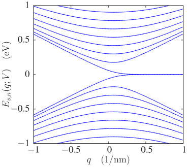
Figure 2: (Color online) The energy spectrum $E_{s,n}(q;V)$ of a zig-zag graphene nanoribbon of width $w=15$ nm in the absence of an external potential, $V=0$.

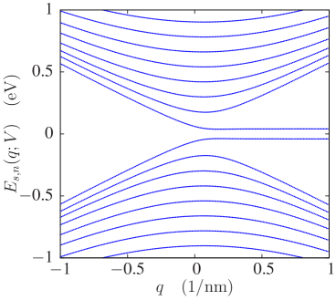
Figure 3: (Color online) The energy spectrum $E_{s,n}(q;V)$ of a zig-zag graphene nanoribbon of width $w=15$ nm in the presence of external electric potentials $V=\pm 0.0403$ eV. The width of the left and right strips ($y_{L}=w-y_{R}$) where the potentials are applied is $2w/5$.

III Results and Discussion

Now we turn to the discussion of the energy spectrum. In Figs. 2-5, we show a numerical evaluation of $f(E;q,V)=0$. In graphene zig-zag nanoribbons, the bulk gap closes due to surface states Fujita et al. (1996); Nakada et al. (1996) at the edges at $y=0$ and $y=w$. This is shown in Fig 2, where part of the energy spectrum $|E_{s,n}(q)|\leq 1.0$ eV as obtained from (9) is plotted for one valley and $V=0$. If we then apply a potential $\pm V$ that affects the eigenstates located at the the zig-zag edges as described above, a gap opens proportional to $V$ until it reaches a maximum value determined by the width $w$ in $y$-direction. Here, we study the symmetric case where $y_{L}=w-y_{R}$. For a finite electric potential $\pm V$, the magnitude of the spectral gap depends on the width of the electrodes, $y_{L}=w-y_{R}$, as long as $y_{L}$ is smaller than the effective width $w_{e}\approx q^{-1}$ of the edge state. Therefore, a much stronger $V$ must be applied to achieve the same spectral gap if $y_{L}<w_{e}$. The energy gap increases with $y_{L}$ and saturates at $y_{L}\gtrsim w_{e}$ for which the energy spectrum becomes independent of $y_{L}$. The latter situation is realized in Figs. 3, 4, and 5, where the steps that define the width of the potential strips are chosen to be at $y_{L}=0.4\,w$ and $y_{R}=0.6\,w$, respectively. If we continue to increase $V$, the gap closes again (see Fig. 5) although the edge states, which can always be identified by their nearly dispersionless eigenenergies, move further apart because they are strongly affected by the external potential. With increasing $V$, the transition point where the bulk state transform into edge states moves to larger $q$.

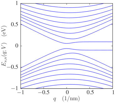
Figure 4: (Color online) The energy spectrum $E_{s,n}(q;V)$ of a zig-zag graphene nanoribbon for external electric potentials $V=\pm 0.0978$ eV. The widths of ribbon and potential strips are as in Fig. 3.

The energy spectrum at $q=0$ can be found for arbitrary potential widths $y_{L}$ and $w-y_{R}$ by putting in (9) $q_{L}=q_{M}=q_{R}=i$. We get

$$E_{s,n}(q=0)=s\frac{\pi}{w}(n+\frac{1}{2})-V\frac{w-y_{L}-y_{R}}{w}.$$ (12)

For $n\gtrsim 1$, the minima of the electron subbands and the maxima of the hole subbands appear not at $q=0$ but at $q\simeq 1/w$. Also, for $2V<\pi\hbar v_{\rm F}/w$ and increasing $q$, the electronic states at $E_{s,0}(q)$ start to become almost dispersionless surface states close to the momentum $q\simeq 1/w$. The corresponding eigenenergies can be calculated in the range $1/w<q<1/a_{0}$, where $a_{0}$ is the lattice constant of the underlying lattice model. A careful evaluation of (9) in the limit $q\to\infty$ yields for the upper ($s=1$) and lower ($s=-1$) state

$$E_{s,0}(1/w<q<1/a_{0})\propto\left\{\begin{array}[]{lll}s|V|(1-e^{-2qy_{L}})&\mathrm{;}&sV>0\\ s|V|(1-e^{-2q(w-y_{R})})&\mathrm{;}&sV<0.\end{array}\right.$$ (13)

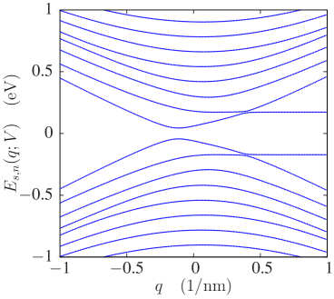
Figure 5: (Color online) The energy spectrum $E_{s,n}(q;V)$ of a zig-zag graphene nanoribbon with electric potentials $V=\pm 0.1725$ eV. A closer inspection of the spectrum shows that the curves do not cross. The widths of ribbon and potential strips are as in Fig. 3.

The appertaining density of states can also be estimated in this limit. It drops from large values at $\pm V$ down to zero at the Dirac point. For $V=0$, however, we get $E_{s,0}(q)=s2qe^{-qw}$ and so the corresponding density of states behaves in the limit of $|Ew|\to 0$ as $\sim|Ew|^{-1}$.

Please note that in the Dirac approximation, the almost dispersionless states at $E_{\pm 1,0}(q)$ seem to be true solutions for all $q\to\infty$. However, if one notices that this model originates from a lattice model, one sees that the nearly dispersionless states merely connect the two valleys at $\mathbf{k}=+\mathbf{K}$ and $\mathbf{k}=-\mathbf{K}$. That means, the Dirac model needs to be supplied with a cut-off ($q_{\rm max}\approx 1/a_{0}$) in order to properly describe the asymptotic ($E\sim 0$) region of the tight-binding (TB) model.

IV Transport, influence of disorder and conclusions

To support our finding of an induced spectral gap obtained within the continuum Dirac-model and to see its influence on the transport properties, we calculate numerically the two-terminal conductance $g(E)$ of narrow graphene zig-zag ribbons applying a transfer-matrix method within a TB-lattice model.Schweitzer and Markoš (2008) Here, semi-infinite leads are attached to both ends of the finite nanoribbon and the electric conductance is defined as usual via the transmission through the entire system (see Ref. Schweitzer and Markoš, 2008 and references therein for details). As an example, the logarithm of the energy dependent $g(E)$ is shown in Fig. 6 for a clean 15 nm narrow nanoribbon with an electric potential $V/t=\pm 0.006$ applied along the edges leading to a transport gap around the Dirac point. Here, $t\approx 2.7$ eV is the nearest-neighbor hopping term in graphene. The conductance exhibits sharp resonances with maxima $g(E)\simeq e^{2}/h$ and decreases down to very small values $\sim 10^{-10}e^{2}/h$ for energies between $\pm 0.006\,t$. The latter is due to tunneling and depends on the length of the sample.

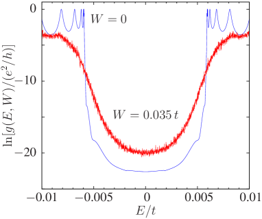
Figure 6: (Color online) The logarithm of the two-terminal conductance $g(E)$ vs. energy $E$ of a perfect (blue curve) narrow zig-zag graphene lattice of 15 nm width in the presence an effective electric potential $V/t=\pm 0.006$ applied along the edges showing a transport gap $\Delta E=2V$. The red curve reflects the influence of additional edge disorder $W/t=0.035$ (see text below).

Fig. 7 shows the dependence of the induced transport gap $\Delta E$ on the effective external potential $V$, and that nicely confirms the linear behavior of our analytical results for small $V$. The transport gap data plotted vs. potential in Fig (7) can be re-scaled by the respective ribbon widths. The outcome of this procedure is, within the given uncertainty of the data, a single fitting curve for all data (not shown). This result can be understood from an evaluation of (9) where one finds for $y_{L}=w-y_{R}$ that the maximal gap appears always at the Dirac point $q=0$. Therefore, Eq. (12) can be used to see that $2E_{1,0}w=\pi$ which together with the observed $1/2\Delta E=V$ relation gives the scaling behavior mentioned above. The maximal transport gap observed in the lattice model agrees within the numerical uncertainty with the spectral gap of both the finite lattice model and the continuum model where $L\to\infty$ was assumed. Recovering the units, we get from (12) and $\hbar v_{F}=3/2tc$, where $c=1.42\times 10^{-10}$ m is the carbon-carbon bond length, that the maximal spectral gap (for $y_{L}=w-y_{R}$) follows the relation

$$E_{\rm max}(w)=\frac{\pi}{w}\hbar v_{\rm F}=\frac{3}{2}\frac{\pi}{w}tc,$$ (14)

leading to $E_{\rm max}\approx 0.12$ eV for $W=15$ nm. We also find in our numerical work that replacing the assumed piece-wise constant effective electric potentials by more realistic smooth potential steps does not modify the results.

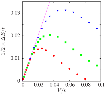
Figure 7: (Color online) The transport gap $\Delta E$ vs. external potential $V$ obtained numerically from the energy dependent two-terminal conductance $g(E)$ of narrow zig-zag graphene lattices having widths 10 nm ($\blacktriangledown$), 15 nm ( ), and 22 nm ($\bullet$), respectively. The straight line is $\Delta E=2V$ and $t\approx 2.7$ eV is the tight-binding hopping energy.

Finally, to check the robustness of this proposed gap opening mechanism against edge disorder, which may arise, e.g., through edge passivation by randomly placed hydrogen atoms that is known to stabilize the edges of pristine zig-zag nanoribbons considerably,Wassmann et al. (2008) we apply a random disorder potential along the border of the ribbon. The eigenvalues are obtained by standard diagonalization of the Hamilton matrix for $L_{x}\times L_{y}$ graphene zig-zag ribbons described by the TB-Hamiltonian defined on a bricklayer latticeSchweitzer and Markoš (2008) with sites $\mathbf{r}$ and nearest neighbor distance $a$

$${\cal H}=\sum_{\mathbf{r}}\epsilon_{\mathbf{r}}c_{\mathbf{r}}^{\dagger}c_{\mathbf{r}}-t\sum_{\langle\mathbf{r}\neq\mathbf{r}^{\prime}\rangle}c_{\mathbf{r}}^{\dagger}c_{\mathbf{r}^{\prime}},$$ (15)

where $\langle\mathbf{r}\neq\mathbf{r}^{\prime}\rangle$ are pairs of those neighboring sites that are mutual connected on the bricklayer. The disorder potentials $\epsilon_{r}$ are uncorrelated random numbers that are non-zero only at the outer sites (different sublattice on left and right edge) along the zig-zag edges of the nanoribbon and uniformly distributed between $\pm W$, where $W$ denotes the disorder strength.

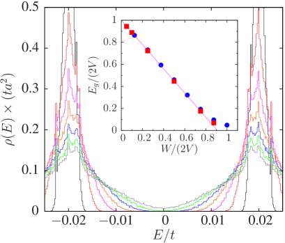
Figure 8: (Color online) The density of states $\rho(E)$ of graphene zig-zag nanoribbons ($L_{x}/a=720$, $L_{y}/a=72$) with external edge potentials $V/t=\pm 0.02$ in the energy interval $-0.025\leq E/t\leq 0.025$ around the Dirac point. One identifies the disorder broadening of the peaks at $E/t=\pm 0.02$, which belong to the eigenstates located along the ribbon edges, for disorder strengths $W/t=$ 0.005 (black narrow peaks), 0.01 (red), 0.015 (magenta), 0.02 (orange), 0.025 (blue), 0.03 (green), and 0.035 (grey broadest peaks). The mean spectral gap $E_{g}$ decreases linearly with increasing disorder strength $W$. This is shown in the inset ($\bullet$) together with additional data for a system of size $L_{x}/a=960$, $L_{y}/a=48$ and $V/t=0.01$ ( ) which all scale onto a single curve $E_{g}=2V-1.1\,W$ almost until the gap closes.

The resulting density of states (DOS) of a 15 nm zig-zag nanoribbon with $L_{x}/a=720$, $L_{y}/a=72$, and $V/t=0.02$, averaged over 1000 disorder realizations, shows a broadening of the DOS-peaks around $E/t=\pm 0.02$ that originate from the edge states (see Fig. 8). With increasing disorder potential strength $W/t=$ 0.005, 0.01, 0.015, 0.02, 0.025, 0.03, and 0.035, the spectral gap decreases linearly. This is seen in the inset of Fig. 8, where the above results are shown together with additional data from a system of size $L_{x}/a=960$, $L_{y}/a=48$ (10 nm ribbon), and $V/t=0.01$. All data points collapse onto the function $E_{g}=2V-1.1W$, which was also observed for other ribbon sizes having widths larger than 7 nm. Therefore, a gap should remain open in experiments when $V$ is tuned to be larger than $0.55\times W$, where $W$ is usually fixed by the sample dependent intrinsic edge disorder. Here, the mean energy gap $E_{g}=1/N_{r}\sum_{i}^{N_{r}}(E_{i}^{+}-E_{i}^{-})$ is defined as the ensemble averaged difference between the smallest positive and the largest negative eigenvalue averaged over $N_{r}$ realizations. For general disorder with box-probability density-distributions $P(\epsilon)$, we find a gap closing relation $E_{g}=2V-\kappa\Gamma_{2}^{1/2}$, where $\Gamma_{2}=\int_{-\infty}^{\infty}\epsilon^{2}P(\epsilon)d\epsilon$ is the second moment of the disorder distribution and $\kappa=1.9$ is an empirical constant.

The influence of edge disorder on the logarithm of the two-terminal conductance, $\ln g(E,W)$ averaged over 100 realizations, is shown in Fig. 6 for a finite lattice of width $L_{y}/a=72$ and length $L_{x}/a=720$. Due to the random edge potentials, the sharp conductance resonances of the clean sample are smoothened out. Yet, a transport gap remains visible even in the case of strong disorder $W=0.035\,t$ when the spectral gap has completely vanished but $g(E)$ still drops six orders of magnitudes from about $g\simeq 0.1\,e^{2}/h$ at $E=0.008\,t$ to $g=10^{-7}e^{2}/h$ at $E=0$. This means that the almost one-dimensional edge states of the clean sample become Anderson localized in the presence of sufficient edge disorder. This notion has been corroborated by an investigation of the respective eigenstates and by calculations of the length and disorder dependence of $g(E)$. Previous studies have reached similar conclusions for nanoribbons with rough edges.Evaldsson et al. (2008); Mucciolo et al. (2009)

In conclusion, we have shown that the application of external electric potentials, covering the area of the electronic edge states that are located along the zig-zag edges of a graphene nanoribbon, can open a tunable spectral gap. Thus, one can convert the metallic behavior into a semiconducting one. For small potentials, the gap increases linearly with the potential strength, reaches a ribbon-width-dependent maximum $\pi\hbar v_{\rm F}/w$ ($\approx$ 0.12 eV for $w=$15 nm) and closes again with further increasing electric potentials. The origin of this effect comes from the sensitivity of the spinorial edge states to electric potentials. Applying distinct external biases to the left and right edge state leads to a different shift of the almost dispersionless edge energies as long as they are not pinned to the Fermi level. Using electric potentials of opposite sign causes the largest energy gap possible. The disorder effects, which may be due to atoms and molecules that saturate the dangling-bonds along the zig-zag edges in real samples, are found to reduce the spectral gap. The latter remains, however, finite as long as $W<1.82V$, where $W$ is a measure of the disorder strength and $V$ the applied effective electric potential. For even larger disorder strengths, a transport gap is still present allowing for reasonable on-off-rations for the electric current. Future experiments will show whether the present results of single particle physics are sufficient for the description of a gap opening by external potentials in graphene zig-zag nanoribbons or if theories that emphasize edge magnetism Son et al. (2006b, a); Jung et al. (2009) due to $e$-$e$ interactions have to be applied.

Note added: During the review procedure, we became aware of a recent paper Bhowmick and Shenoy (2010) by Bhowmick and Shenoy that addresses a spectral gap opening induced by external $\delta$-like potentials placed along the edges of graphene zig-zag ribbons. This specific potential choice represents a special case contained in our model.

References

- Castro Neto et al. (2008) A. H. Castro Neto, F. Guinea, N. M. R. Peres, K. S. Novoselov, and A. K. Geim, Rev. Mod. Phys. 81, 109 (2008).
- Beenakker (2008) C. W. J. Beenakker, Rev. Mod. Phys. 80, 1337 (2008).
- Castro Neto (2010) A. H. Castro Neto, Materials Today 13, 12 (2010).
- Giovannetti et al. (2007) G. Giovannetti, P. A. Khomyakov, G. Brocks, P. J. Kelly, and J. van den Brink, Phys. Rev. B 76, 073103 (2007).
- Gui et al. (2008) G. Gui, J. Li, and J. Zhong, Phys. Rev. B 78, 075435 (2008).
- Pereira et al. (2009) V. M. Pereira, A. H. Castro Neto, and N. M. R. Peres, Phys. Rev. B 80, 045401 (2009).
- Han et al. (2007) M. Y. Han, B. Özyilmaz, Y. Zhang, and P. Kim, Phys. Rev. Lett. 98, 206805 (2007).
- Lin et al. (2008) Y.-M. Lin, V. Perebeinos, Z. Chen, and P. Avouris, Phys. Rev. B 78, 161409 (2008).
- Novikov (2007) D. S. Novikov, Phys. Rev. Lett. 99, 056802 (2007).
- Fujita et al. (1996) M. Fujita, K. Wakabayashi, K. Nakada, and K. Kusakabe, J. Phys. Soc. Japan 65, 1920 (1996).
- Nakada et al. (1996) K. Nakada, M. Fujita, G. Dresselhaus, and M. S. Dresselhaus, Phys. Rev. B 54, 17954 (1996).
- Wakabayashi et al. (2009) K. Wakabayashi, Y. Takane, M. Yamamoto, and M. Sigrist, New Journal of Physics 11, 095016 (2009).
- Sasaki et al. (2006) K. Sasaki, S. Murakami, and R. Saito, J. Phys. Soc. Jpn. 75, 074713 (2006).
- Sasaki et al. (2008) K. Sasaki, M. Suzuki, and R. Saito, Phys. Rev. B 77, 045138 (2008).
- Son et al. (2006a) Y.-W. Son, M. L. Cohen, and S. G. Louie, Phys. Rev. Lett. 97, 216803 (2006a).
- Son et al. (2006b) Y.-W. Son, M. L. Cohen, and S. G. Louie, Nature 444, 347 (2006b).
- Solér et al. (2002) J. M. Solér, E. Artacho, J. D. Gale, A. Garciá, J. Junquera, P. Ordejón, and D. Sánchez-Portal, J. Phys.: Condens. Matter 14, 2745 (2002).
- Kan et al. (2007) E. Kan, Z. Li, J. Yang, and J. G. Hou, Appl. Phys. Lett. 91, 243116 (2007).
- Jung et al. (2009) J. Jung, T. Pereg-Barnea, and A. H. MacDonald, Phys. Rev. Lett. 102, 227205 (2009).
- Kunstmann et al. (2011) J. Kunstmann, C. Özdoğan, A. Quandt, and H. Fehske, Phys. Rev. B 83, 045414 (2011).
- Ando et al. (1998) T. Ando, T. Nakanishi, and R. Saito, J. Phys. Soc. Jpn. 67, 2857 (1998).
- Katsnelson et al. (2006) M. I. Katsnelson, K. S. Novoselov, and A. K. Geim, Nature Physics 2, 620 (2006).
- Gusynin and Sharapov (2005) V. P. Gusynin and S. G. Sharapov, Phys. Rev. Lett. 95, 146801 (2005).
- Ando (2007) T. Ando, Physica E 40, 213 (2007).
- Brey and Fertig (2006) L. Brey and H. A. Fertig, Phys. Rev. B 73, 235411 (2006).
- Schweitzer and Markoš (2008) L. Schweitzer and P. Markoš, Phys. Rev. B 78, 205419 (2008).
- Wassmann et al. (2008) T. Wassmann, A. P. Seitsonen, A. M. Saitta, M. Lazzeri, and F. Mauri, Phys. Rev. Lett. 101, 096402 (2008).
- Evaldsson et al. (2008) M. Evaldsson, I. V. Zozoulenko, H. Xu, and T. Heinzel, Phys. Rev. B 78, 161407 (2008).
- Mucciolo et al. (2009) E. R. Mucciolo, A. H. Castro Neto, and C. H. Lewenkopf, Phys. Rev. B 79, 075407 (2009).
- Bhowmick and Shenoy (2010) S. Bhowmick and V. B. Shenoy, Phys. Rev. B 82, 155448 (2010).