Backflow correlations in the Hubbard model: an efficient tool for the metal-insulator transition and the large-$U$ limit

Abstract

We show that backflow correlations in the variational wave function for the Hubbard model greatly improve the previous results given by the Slater-Jastrow state, usually considered in this context. We provide evidence that, within this approach, it is possible to have a satisfactory connection with the strong-coupling regime. Moreover, we show that, for the Hubbard model on the lattice, backflow correlations are essentially short range, inducing an effective attraction between empty (holons) and doubly occupied sites (doublons). In presence of frustration, we report the evidence that the metal to Mott-insulator transition is marked by a discontinuity of the double occupancy, together with a similar discontinuity of the kinetic term that does not change the number of holons and doublons, while the other kinetic terms are continuous across the transition. Finally, we show the estimation of the charge gap, obtained by particle-hole excitations à la Feynman over the ground-state wave function.

I Introduction

Backflow correlations were introduced by Feynman and Cohen feynman in order to obtain an accurate description of the excitation spectrum of liquid He⁴. Indeed, by accounting for these correlations, it was possible to have a marked improvement in the one-phonon dispersion curve and obtain an accurate description of the roton excitations. Indeed, it was realized that a picture of independent elementary excitations had to be extended to account for their interactions. Essentially, the current associated with a Feynman excitation involves a contribution from the backflow of the fluid around it. Feynman and Cohen showed that, in the simplest case of a particle tearing through the liquid at a given velocity, the pattern of induced longitudinal current far away from the particle has a dipolar form. feynman Then, the concept of backflow has been extended to weakly-correlated electron systems, where it turned out to be crucial for improving the description of the electron gas in two and three dimensions, in particular, for correlation energies and pair distribution functions. ceperley Further applications concerned metallic Hydrogen holzmann and small atoms or molecules, molecules where significant improvements in the total energy have been obtained.

Very recently, backflow correlations have been successfully applied to strongly-correlated electron systems, such as the Hubbard model and its generalizations to include frustrating terms, improving the variational wave functions used so far to approximate the exact ground state. In particular, in presence of frustration (e.g., for the $t{-}t^{\prime}$ Hubbard model on the square tocchio1 and the triangular lattices tocchio2 ) a spin-liquid phase has been stabilized only thanks to backflow correlations. This new term allowed us also to observe a renormalization of the underlying Fermi surface to perfect nesting at the metal-insulator transition. tocchio3 Backflow correlations have been also recently applied to the infinite-$U$ Hubbard model to study the stability of the Nagaoka ferromagnetism. carleo

When compared to former variational wave functions for frustrated Hubbard models, fazekas (short-range) backflow correlations significantly improved the description of ground-state properties with respect to density-density Jastrow factors capello and holon-doublon binding factors. yoko However, also in presence of backflow terms, the long-range Jastrow factor is still a fundamental ingredient of the wave function in order to describe the metal-insulator transition occurring at a finite value of the ratio between the electron-electron repulsion $U$ and the hopping integral $t$.

In this paper, we show the accuracy of backflow correlations and compare them with the $S$-matrix (i.e., strong-coupling) expansion. macdonald ; gros87 The latter approach becomes exact for $U/t\to\infty$ and define an iterative procedure which results in an expansion in powers of $t/U$. As a consequence, the (exact) wave function will be an admixture of electronic configurations with weights proportional to $(t/U)^{n}$, where $n$ is the number of doubly-occupied sites. Unfortunately, dealing with such a state is a difficult task, and, at present, only few attempts have been pursued in this direction. baeriswyl On the contrary, our approach based upon backflow correlations define a many-body wave function that can be easily treated by standard Monte Carlo methods. Most importantly, it remains accurate also for intermediate electron-electron repulsion, allowing a precise description of the physics down to the metal-insulator transition. tocchio1 ; tocchio2 Here, we show that the energy gain due to backflow correlations in the insulating phase is mainly related to a better description of the local hopping processes changing the total numbers of holon-doublon couples. We discuss the extension of backflow correlations to long-range distances and how the behavior of the Jastrow factor is affected by the presence of backflow correlations. We present the results both for one and two dimensions, with the variational wave function containing no magnetic terms. Finally, we discuss also how the variational method allows us to calculate the charge gap in the insulating phase and present results for the one-dimensional case.

The paper is organized as follows: in Sec. II, we introduce the Hamiltonian and we describe our variational wave function; in Sec. III, we give a short review of the strong-coupling approach based upon the $S$ matrix, to give a justification of the backflow terms; in Sec. IV, we describe the backflow correlations; in Sec. V, we present some results for the metal-insulator transition and the insulating phase; finally, in Sec. VI, we draw our conclusions.

II Model and variational wave function

We consider the Hubbard model with extended hopping in one-dimensional (1D) and two-dimensional (2D) square lattices.

$${\cal H}=-\sum_{i,j,\sigma}t_{ij}c^{\dagger}_{i,\sigma}c^{\phantom{\dagger}}_{j,\sigma}+U\sum_{i}n_{i,\uparrow}n_{i,\downarrow},$$ (1)

where $c^{\dagger}_{i,\sigma}$ ($c^{\phantom{\dagger}}_{i,\sigma}$) denotes the creation (annihilation) operator of one electron on site $i$ with spin $\sigma=\uparrow,\downarrow$, $n_{i,\sigma}=c^{\dagger}_{i,\sigma}c^{\phantom{\dagger}}_{i,\sigma}$ is the electron density, $t_{ij}$ the hopping parameters, and $U$ the on-site Coulomb repulsion. In the following, we will consider nearest- and next-nearest-neighbor hoppings that will be respectively denoted by $t$ and $t^{\prime}$ in 2D and by $t_{1}$ and $t_{2}$ in 1D. We will focus our attention on the half-filled case with $L$ electrons on $L$ sites.

Both metallic and insulating phases can be constructed in a variational approach. In a first step, one constructs uncorrelated wave functions given by the ground state $|\rm{BCS}\rangle$ of a superconducting Bardeen-Cooper-Schrieffer (BCS) Hamiltonian, grosbcs ; zhang88

$${\cal H}_{\rm{BCS}}=\sum_{q,\sigma}\epsilon_{q}c^{\dagger}_{q,\sigma}c^{\phantom{\dagger}}_{q,\sigma}+\sum_{q}\Delta_{q}c^{\dagger}_{q,\uparrow}c^{\dagger}_{-q,\downarrow}+\rm{h.c.},$$ (2)

where both the free-band dispersion $\epsilon_{q}$ and the pairing amplitude $\Delta_{q}=\Delta_{-q}$ are variational functions. We use the parametrization

$$\epsilon_{q} = -2\tilde{t}[\cos(q_{x})+\cos(q_{y})]-4\tilde{t}^{\prime}\cos(q_{x})\cos(q_{y})-\mu$$

$$\Delta_{q} = \Delta_{1}[\cos(q_{x})-\cos(q_{y})],$$

on the 2D square lattice and the parametrization

$$\epsilon_{q} = -2\tilde{t}_{1}\cos(q)-2\tilde{t}_{2}\cos(2q)-\mu$$

$$\Delta_{q} = \Delta_{1}\cos(q)+\Delta_{2}\cos(2q)+\Delta_{3}\cos(3q),$$

on the 1D lattice. The next-nearest-neighbor hopping parameters, as well as the effective chemical potential $\mu$ and the pairing fields, are variational parameters to be optimized. $\tilde{t}=\tilde{t}_{1}=1$ is kept fixed to set the energy scale. The correlated state $|\Psi\rangle$, without backflow, is then given by

$$|\Psi\rangle={\cal J}|\textrm{BCS}\rangle,$$ (3)

where

$${\cal J}=\exp(-\frac{1}{2}\sum_{i,j}v_{i,j}n_{i}n_{j}),$$ (4)

is a density-density Jastrow factor (including the on-site Gutzwiller term $v_{i,i}$), with the $v_{i,j}$ being optimized independently for every distance $|i-j|$. Notably, within this kind of wave function, it is possible to obtain a pure (i.e., non-magnetic) Mott insulator by considering a sufficiently strong Jastrow factor, capello i.e., $v_{q}\sim 1/q^{2}$ ($v_{q}$ being the Fourier transform of $v_{i,j}$) and a metallic state whenever $v_{q}\sim 1/q$. In fact, it has been shown that $v_{q}\sim 1/q^{2}$ is necessary to have a vanishing quasi-particle weight in fermionic models, capello2 or to have a vanishing condensate fraction in bosonic models. capello3 Nonetheless, much more difficult is to demonstrate by numerical simulations that such a Jastrow term is sufficient to obtain exponential correlations, which are suitable for a fully gapped Mott insulator.

As recently shown, tocchio1 the projected BCS state $|\Psi\rangle$ can be rather poor for large on-site interactions, in presence of frustration. In order to overcome this limitation, a further improvement of the variational wave function is needed. One possibility (which is discussed in the next section) is to consider the strong-coupling approach, based upon the $S$-matrix expansion. macdonald ; gros87 Unfortunately, this method cannot be easily handled by quantum Monte Carlo simulations on large systems. However, an alternative, but somewhat related, approach may be defined in terms of backflow correlations, which is stable and accurate even for large system sizes.

III The large-$U$ limit and the $S$-matrix expansion

Let us consider the limit of $U/t\to\infty$. Here, there are no doublons and the wave function can be written as $|\Psi_{\infty}\rangle={\cal P}_{G}|\textrm{MF}\rangle$, where the full Gutzwiller projector ${\cal P}_{G}=\prod_{i}(1-n_{i,\uparrow}n_{i,\downarrow})$ removes all double occupancies, while $|\textrm{MF}\rangle$ denotes an uncorrelated mean-field state, such as the $|\textrm{BCS}\rangle$ state introduced in the previous section. Then, the strong-coupling approach allows one to define and construct a variational wave function for the Hubbard model at large but finite values of $U/t$ by

$$|\Psi_{S}\rangle=e^{-iS}|\Psi_{\infty}\rangle,$$ (5)

where the operator $S$ can be determined by using a recursive scheme. At the lowest order in $t/U$, $iS=(T^{+}-T^{-})/U$, where $T^{+}$ and $T^{-}$ correspond to the kinetic terms that increase and decrease the number of doubly occupied sites by one: macdonald ; gros87

$$T^{+} = -\sum_{i,j,\sigma}t_{ij}n_{i,-\sigma}c^{\dagger}_{i,\sigma}c^{\phantom{\dagger}}_{j,\sigma}(1-n_{j,-\sigma})$$ (6)

$$T^{-} = -\sum_{i,j,\sigma}t_{ij}(1-n_{i,-\sigma})c^{\dagger}_{i,\sigma}c^{\phantom{\dagger}}_{j,\sigma}n_{j,-\sigma}.$$ (7)

However, the wave function of Eq. (5) is hard to handle (both analytically and numerically), since $S$ is non-diagonal in the basis where the electrons have defined positions in the lattice (in contrast to the Jastrow term, which is diagonal). In the large-$U$ limit, one can further expand the exponential and obtain:

$$|\Psi_{S}\rangle\simeq(1-iS)|\Psi_{\infty}\rangle.$$ (8)

This state has non-vanishing weights only for electronic configurations with zero or one doublon. Indeed, $|\Psi_{\infty}\rangle$ does not contain doubly occupied sites and $S$ may generate at most one doublon. Therefore, after the expansion of the exponent, the wave function is no longer size consistent. Let us see what can be learned from this strong-coupling approach. Suppose that an electronic configuration $|x_{0}\rangle$ has no doubly occupied sites, then, since ${\cal P}_{G}|x_{0}\rangle=|x_{0}\rangle$, from Eq. (8) we have that:

$$\langle x_{0}|\Psi_{S}\rangle=\langle x_{0}|\textrm{MF}\rangle;$$ (9)

on the other hand, if the configuration $|x_{1}\rangle$ contains one doublon (with the holon in one of its neighboring sites), we have that:

$$\langle x_{1}|\Psi_{S}\rangle=\pm\frac{t}{U}\langle y_{0}|\textrm{MF}\rangle\pm\frac{t}{U}\langle z_{0}|\textrm{MF}\rangle,$$ (10)

where $|y_{0}\rangle$ and $|z_{0}\rangle$ are the (only) two possible configurations with no doubly occupied sites that are connected to $|x_{1}\rangle$ by $S$; signs depend upon the convention used for labeling electronic configurations. Therefore, the weight of a configuration with one doublon is related to the weight of two configurations without doublons (times $t/U$).

This procedure for defining a variational wave function is exact for $U\gg t$, when at most one doublon is present in the electronic configurations; however, one is mostly interested into the case where an arbitrary number of doublons and holons are present (relevant for the generic case with $U\sim t$), and the straightforward generalization of this formalism becomes much more elaborated and difficult to implement in numerical calculations.

IV Backflow correlations

IV.1 Definition of backflow terms

As introduced in Ref. tocchio1, , backflow correlations modify the single-particle eigenstates $\phi_{k}(\bm{r}_{i,\sigma})$ of the mean-field Hamiltonian, like for example ${\cal H}_{\textrm{BCS}}$ defined in Eq. (2), according to the electronic configuration on the lattice:

$$\phi_{k}^{b}(\bm{r}_{i,\sigma}) \equiv \tilde{\epsilon}\phi_{k}(\bm{r}_{i,\sigma})+\eta_{1}\sum_{j\textrm{n.n.}i}D_{i}H_{j}\phi_{k}(\bm{r}_{j,\sigma})$$ (11)

$$+ \eta_{2}\sum_{j\textrm{n.n.n.}i}D_{i}H_{j}\phi_{k}(\bm{r}_{j,\sigma}),$$

where $\tilde{\epsilon}=\epsilon$ if the site $i$ is doubly occupied and is surrounded by at least one empty site, while $\tilde{\epsilon}=1$ in all the other cases. Here $\epsilon,\eta_{l},(l=1,2)$ are variational parameters to be optimized, $D_{i}=n_{i,\uparrow}n_{i,\downarrow}$ and $H_{i}=h_{i,\uparrow}h_{i,\downarrow}$, with $h_{i,\sigma}=1-n_{i,\sigma}$. Moreover, the shorthand notations n.n. and n.n.n. indicate nearest- and next-nearest-neighbor sites, respectively. In this way, already the determinant part of the wave function includes correlation effects, strongly improving the accuracy of the many-body state. When backflow correlations are included in the Slater determinant, the state will be denoted by $|\Psi^{b}\rangle$. This is a substantial improvement with respect to Jastrow factors, where electron-electron correlation is included only via a multiplicative term (i.e., giving a “classical” potential acting on the electronic configuration).

The results for the $S$-matrix expansion may be compared with the ones of backflow correlations for large electron-electron interactions, namely when at most one doublon is present. Indeed, whenever no doubly-occupied sites are present, we have that

$$\langle x_{0}|\Psi^{b}\rangle=\langle x_{0}|\textrm{MF}\rangle$$ (12)

(where we dropped the Jastrow weight, since all sites are singly occupied, and it represents a multiplicative constant). We discuss now the case of a single doublon and note that the backflow corrections (11) are valid for both up- and down-spin orbitals. We consider here, for simplicity, only nearest-neighbor backflow terms, with parameters $\epsilon$ and $\eta=\eta_{1}$, and obtain:

$$\langle x_{1}|\Psi^{b}\rangle= {\cal J}(x_{1})\left[\pm\eta\epsilon\langle y_{0}|\textrm{MF}\rangle\pm\eta\epsilon\langle z_{0}|\textrm{MF}\rangle\right.$$

$$+ \left.\epsilon^{2}\langle x_{1}|\textrm{MF}\rangle+\eta^{2}\langle{\tilde{x}_{1}}|\textrm{MF}\rangle\right],$$ (13)

where, in analogy with the $S$-matrix expansion, backflow correlations act on configurations with doubly occupied sites (i.e., $|x_{1}\rangle$), transferring some weight to configurations without doubly-occupied sites ($|y_{0}\rangle$ and $|z_{0}\rangle$ are the same two configurations that appear in the strong-coupling expansion); in addition there is some weight also coming from configurations with one holon-doublon couple (i.e., the original configuration $|x_{0}\rangle$ and a configuration where the two electrons of the doubly-occupied site have been transferred to the empty site $|{\tilde{x}}_{1}\rangle$). The signs of the second and third terms of Eq. (IV.1) are the same as the ones appearing in Eq. (10). The relative weights of the admixture in Eq. (IV.1) is controlled by the variational parameters $\eta$ and $\epsilon$.

Therefore, our way to define the backflow correlations is strictly related to the strong-coupling approach; moreover, it allows us to consider many couples of holons and doublons, with a moderate computational cost, since they just re-define the Slater determinant of the wave function. Finally, we would like to mention that the backflow wave function, on the contrary to the strong-coupling approach of Eqs. (8), (9), and (10), is size consistent.

The terms in Eq. (11) are the dominant contributions to the backflow operator, having a qualitative influence on the properties of the correlated wave functions. In addition, we can also take into account further terms that are useful in the intermediate-coupling regime and correspond to all possible hopping processes:

$$\phi_{k}^{b}(\bm{r}_{i,\sigma})\equiv\tilde{\epsilon}_{i}\phi_{k}(\bm{r}_{i,\sigma})+\eta_{1}\sum_{j\textrm{n.n.}i}D_{i}H_{j}\phi_{k}(\bm{r}_{j,\sigma})+$$

$$\eta_{2}\sum_{j\textrm{n.n.n.}i}D_{i}H_{j}\phi_{k}(\bm{r}_{j,\sigma})+$$

$$\beta_{1}\sum_{j\textrm{n.n.}i}n_{i,\sigma}h_{i,-\sigma}n_{j,-\sigma}h_{j,\sigma}\phi_{k}(\bm{r}_{j,\sigma})+$$

$$\beta_{2}\sum_{j\textrm{n.n.n.}i}n_{i,\sigma}h_{i,-\sigma}n_{j,-\sigma}h_{j,\sigma}\phi_{k}(\bm{r}_{j,\sigma})+$$

$$\gamma_{1}\sum_{j\textrm{n.n.}i}\left(D_{i}n_{j,-\sigma}h_{j,\sigma}+n_{i,\sigma}h_{i,-\sigma}H_{j}\right)\phi_{k}(\bm{r}_{j,\sigma})+$$

$$\gamma_{2}\sum_{j\textrm{n.n.n.}i}\left(D_{i}n_{j,-\sigma}h_{j,\sigma}+n_{i,\sigma}h_{i,-\sigma}H_{j}\right)\phi_{k}(\bm{r}_{j,\sigma}),$$ (14)

where, in addition to $\epsilon$ and $\eta_{l}$, $\beta_{l},\gamma_{l}(l=1,2)$ are variational parameters to be optimized. All results presented here are obtained by fully incorporating the backflow corrections and optimizing individually sorella every variational parameter in $\epsilon_{q}$ and $\Delta_{q}$ of Eq. (2), in the Jastrow factor $\cal J$ of Eq. (4), as well as for the backflow corrections.

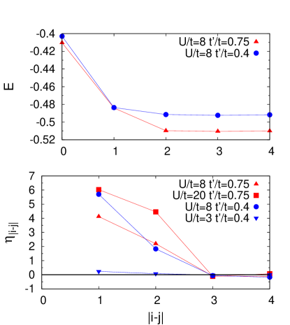
Figure 1: (Color online) Upper panel: Ground-state energy as a function of the range of backflow parameters on the 2D square lattice for $t^{\prime}/t=0.4$ and $0.75$ at $U/t=8$. Range equal to zero corresponds to no backflow correlations in the wave function. Lower panel: Optimized backflow parameters $\eta_{|i-j|}$ as a function of the distance $|i-j|$. Results for $U/t=3$ and $t^{\prime}/t=0.4$ correspond to a metallic state, the others to insulating states. Data are shown for a lattice with $L=98$ sites.

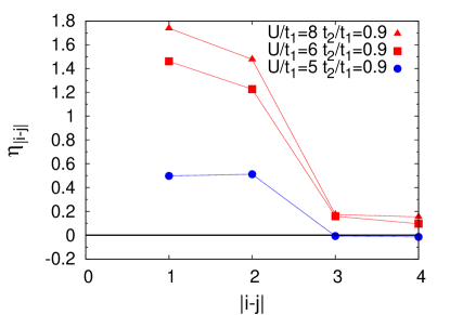
Figure 2: (Color online) Optimized backflow parameters $\eta_{|i-j|}$ as a function of the distance $|i-j|$ for the 1D lattice. The point at $U/t_{1}=5$ lies in the metallic phase, while the other points are located in the insulating region of the phase diagram. Data are shown for a lattice with $L=120$ sites.

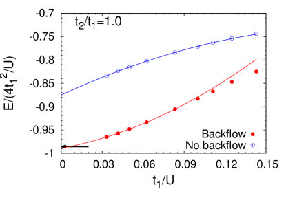
Figure 3: (Color online) The energy (in unit of $4t_{1}^{2}/U$), as a function of $t_{1}/U$, for the 1D Hubbard model with $t_{2}/t_{1}=1$. Filled (empty) circles denote the results with (without) backflow correlations. The DMRG energy of the corresponding Heisenberg model with $J_{2}/J_{1}=1$ is shown by an arrow. chitra Data are presented for a $L=120$ lattice size.

IV.2 Long-range correlations

We consider now the extension of the backflow parameters to further distances. In practice, we allow in Eqs. (11) and (IV.1) different backflow parameters $\eta_{|i-j|},\beta_{|i-j|},\gamma_{|i-j|}$ for every distance of the lattice. We present the results in Fig. 1 for the frustrated 2D square lattice. Here, it is clear that all backflow parameters are irrelevant for all distances larger than few lattice spacing; in particular, they are vanishing for all distances not connected by the hopping amplitude. Most importantly, a remarkable gain in energy is obtained only by a suitable optimization of the backflow parameters up to second neighbors, while poor results are obtained when there is no backflow (or its range is smaller than the one of the hopping). These results suggest that backflow correlations are indeed necessary to successfully describe the effect of frustrating couplings. Furthermore, we show in Fig. 2 the behavior of $\eta_{|i-j|}$ for the 1D lattice up to the fourth distance. Also in this case, the optimized backflow parameters become much smaller for distances not connected by the hopping amplitude.

The effect of backflow correlations in the large $U$ limit is presented in Fig. 3, where energies for large $U/t_{1}$ are shown for the frustrated 1D lattice with $t_{2}/t_{1}=1$. Only the presence of backflow correlations in the wave function allows for a proper extrapolation to the Heisenberg limit. Here, the energy of the Heisenberg model is provided by density-matrix renormalization group (DMRG) calculations, chitra which are numerically exact for 1D models.

In order to assess the accuracy of backflow correlations, we compare the energies obtained within the variational Monte Carlo (VMC) approach of Sec. II with the data obtained by means of Green’s Function Monte Carlo (GFMC) within the fixed-node approximation. gfmc This approach systematically improves the variational wave function, extracting the best ground-state approximation with the same nodes of the starting variational ansatz. The data presented in Table 1, for the insulating phase of the frustrated square lattice, show that the variational energy, in presence of backflow correlations, is lower than the GFMC energy, when the starting variational ansatz does not include the backflow term. This means that backflow correlations are necessary in order to properly describe the ground-state wave function of the frustrated model, capturing its correct signs. In Table 2, we show also data for the unfrustrated square lattice with $t^{\prime}=0$. Here, backflow correlations still strongly improve the accuracy of the variational ansatz, but are less crucial in reproducing the correct signs of the ground-state wave functions. Indeed, for $t^{\prime}=0$, the signs of the $|\Psi\rangle={\cal J}|\textrm{BCS}\rangle$ wave function become exact in the limit $U/t\to\infty$ (e.g., the GFMC results with or without backflow correlations are very close for large $U/t$).

Table 1: Ground-state energies for the Hubbard model on the square lattice with $t^{\prime}/t=0.75$ and $L=162$, obtained by means of variational (VMC) and Green’s Function Monte Carlo (GFMC) methods. Data are shown both in presence of and without backflow correlations.

$U/t$	VMC NO backflow	GFMC NO backflow
8	-0.4048(1)	-0.5072(3)
10	-0.3409(1)	-0.4223(3)
12	-0.2970(1)	-0.3617(2)
16	-0.2373(1)	-0.2816(2)
$U/t$	VMC backflow	GFMC backflow
8	-0.5073(1)	-0.5307(2)
10	-0.4282(1)	-0.4455(2)
12	-0.3704(1)	-0.3831(2)
16	-0.2901(1)	-0.2976(1)

Table 2: The same as in Table 1, but with $t^{\prime}=0$.

$U/t$	VMC NO backflow	GFMC NO backflow
6	-0.5307(1)	-0.6444(1)
8	-0.3955(1)	-0.5045(2)
10	-0.3353(1)	-0.4203(3)
12	-0.2930(1)	-0.3634(3)
$U/t$	VMC backflow	GFMC backflow
6	-0.5961(1)	-0.6448(3)
8	-0.4803(1)	-0.5152(3)
10	-0.4022(1)	-0.4278(2)
12	-0.3451(1)	-0.3651(2)

IV.3 Effect of backflow terms on the Jastrow factor

Here, we would like to discuss the effect of the backflow corrections on the behavior of the Jastrow factors across the metal-insulator transition. As shown in Fig. 4, the metallic phase is characterized by $v_{q}\sim 1/q$, while the insulating phase exhibits a $v_{q}\sim 1/q^{2}$ behavior. A further logarithmic divergence at $q\to 0$ is expected to occur in 2D. capello2 ; capello3 More details on the relation between the Jastrow factor and the conduction properties may be found in Appendix A. The presence of backflow correlations in the wave function strongly reduces the strength of the Jastrow factor in the insulating phase, even if a $v_{q}\sim 1/q^{2}$ behavior is always necessary in order to induce a metal-insulator transition at a finite $U/t$. Indeed, a variational wave function including only a local (soft) Gutzwiller factor $P=\exp(-v\sum_{i}n_{i,\uparrow}n_{i,\downarrow})$ and backflow correlations is found always in the metallic phase.

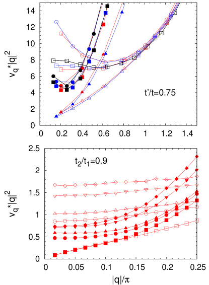
Figure 4: (Color online) Upper panel: Fourier transform of the optimized Jastrow factor $v_{q}$ multiplied by $|q|^{2}$ as a function of $|q|$, along the $(1,1)$ direction of the Brillouin zone of the square lattice, at $t^{\prime}/t=0.75$ for $U/t=7$ (triangles), $U/t=8$ (squares) and $U/t=10$ (circles). Full (empty) symbols refer to the presence (absence) of backflow correlations, while different colors correspond to different lattice sizes: red ($L=98$), blue ($L=162$), black ($L=242$). Lower panel: The same quantity for a 1D lattice with $t_{2}/t_{1}=0.9$. Data are shown for $U/t_{1}=5.4$ (squares), $U/t_{1}=5.6$ (circles), $U/t_{1}=6$ (up-triangles), $U/t_{1}=8$ (down-triangles) and $U/t_{1}=10$ (diamonds) on a $L=120$ lattice size. Full (empty) symbols refer to the presence (absence) of backflow correlations.

V Metal-insulator transition and the insulating phase

Backflow correlations are a powerful tool to describe the whole insulating phase, from the large-$U$ limit down to the metal-insulator transition. In the following, we consider the density of doubly occupied sites $D=1/L\langle\sum_{i}n_{i,\uparrow}n_{i,\downarrow}\rangle$, which is proportional to the interaction energy per site. In addition, we split the kinetic energy into two different parts and we compute them separately: ${\cal K}_{0}$ is the part where the hopping process does not change the total number of holon-doublon couples, while ${\cal K}_{\pm}$ denotes the contributions where one holon-doublon couple is created or destroyed (see Fig. 5).

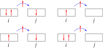
Figure 5: (Color online) Upper raw: Hopping terms of a spin up electron from site $i$ to site $j$ that contribute to ${\cal K}_{0}$. Lower raw: hopping terms of a spin up electron from site $i$ to site $j$ that contribute to ${\cal K}_{\pm}$. Lattice sites $i$ and $j$ are represented as boxes and spin up/down electrons inside them represent the electronic configurations.

The results for $D$ and the kinetic terms are presented in Figs. 6, 7 and 8 as a function of $U$ for the frustrated square lattice with $t^{\prime}/t=0.75$, the unfrustrated one with $t^{\prime}=0$, and the 1D lattice with $t_{2}/t_{1}=0.9$, respectively. The effect of backflow can be clearly seen in the behavior of ${\cal K}_{\pm}$, which is systematically improved, especially in the insulating phase. This trend can be understood by looking at Eq. (11): as long as a holon-doublon couple is formed, backflow correlations favor its recombination into single-occupied sites, increasing the part of the kinetic energy that changes the total number of holon-doublon couples. Moreover, the effect of backflow correlations is particularly strong close to the metal-insulator transition, where the increasing of the holon-doublon recombination washes out the jump in ${\cal K}_{\pm}$. On the contrary, the behavior of ${\cal K}_{0}$ shows a suppression in presence of backflow correlations, since hopping terms that does not change the total number of holon-doublon couples contribute less to the total energy. We want to point out that, in presence of frustration, ${\cal K}_{0}$ exhibits a clear jump at the metal-insulator transition, similarly to the double occupation $D$, both for the square (see Fig. 6) and the 1D lattice (see Fig. 8). Instead, for the unfrustrated square lattice, the jump vanishes and the metal-insulator transition is characterized only by an inflection point (see Fig. 7).

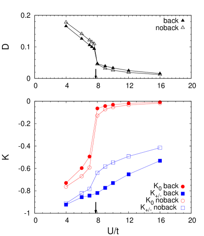
Figure 6: (Color online) Upper panel: Density of doubly occupied sites $D$ as a function of $U/t$. Lower panel: ${\cal K}_{0}$ (circles) and ${\cal K}_{\pm}$ (squares) as a function of $U/t$. Full (empty) symbols refer to the presence (absence) of backflow correlations in the wave function. The metal-insulator transition is marked by an arrow. Data refer to a frustrated square lattice with $t^{\prime}/t=0.75$ and $L=162$.

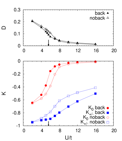
Figure 7: (Color online) The same as in Fig. 6, but for $t^{\prime}=0$.

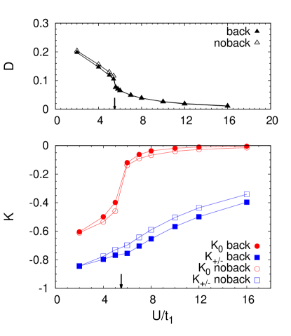
Figure 8: (Color online) The same as in Fig. 6, but for a 1D lattice with $t_{2}/t_{1}=0.9$ and $L=120$.

Finally, we would like to discuss how the variational method allows us to estimate the charge gap in the insulating phase, by assessing the particle-hole excitations over the variational state. This is possible by considering just ground-state expectation values, without directly calculating energy differences. Indeed, within the context of the single-mode approximation (SMA), which was proposed for the liquid Helium feynman2 and further applied to fermionic systems, girvin ; overhauser it is possible to find a relation between the particle-hole excitation energy and the static structure factor $N(q)=\langle n_{-q}n_{q}\rangle$ where $n_{q}=1/\sqrt{L}\sum_{r,\sigma}\textrm{e}^{iqr}n_{r,\sigma}$ is the Fourier transform of the particle density. Indeed, a variational ansatz of the lowest energy state $|\Psi_{q}\rangle$, with a given momentum $q$, can be obtained by applying $n_{q}$ to the ground state wave function $|\Psi\rangle$ (or one approximation for it), namely:

$$|\Psi_{q}\rangle=n_{q}|\Psi\rangle.$$ (15)

The charge gap for the limit $q\to 0$ is then derived in Appendix B and results:

$$E_{q}=-\frac{1}{2\textrm{d}}\left(\lim_{q\to 0}\frac{|q|^{2}}{N(q)}\right)\left[(\Delta r_{1})^{2}{\cal K}_{1}+(\Delta r_{2})^{2}{\cal K}_{2}\right],$$ (16)

where d is the dimensionality, ${\cal K}_{1}$ and ${\cal K}_{2}$ are the nearest- and the next-nearest-neighbor kinetic energy per site, while $\Delta r_{1}$ and $\Delta r_{2}$ are the distances between nearest- and next-nearest-neighbors on the lattice (e.g., $\Delta r_{1}=1$ and $\Delta r_{2}=2$ or $\sqrt{2}$ on the 1D or 2D square lattice).

The metallic phase is characterized by $N(q)\sim q$ for $q\to 0$, which implies a vanishing gap for particle-hole excitations. On the contrary, in the insulating phase, $N(q)\sim q^{2}$ for $q\to 0$, enclosing the fact that the charge gap is finite.

In Fig. 9, we show the gap for $q\to 0$ for the 1D Hubbard model with $t_{2}/t_{1}=0.9$. The gap closes at the metal-insulator transition, as expected, and grows up linearly with $U$ for large values of $U/t_{1}$. For comparison, we also show the same gap in the case $t_{2}=0$ (where a Mott insulating state takes place for infinitesimal values of $U/t_{1}$).

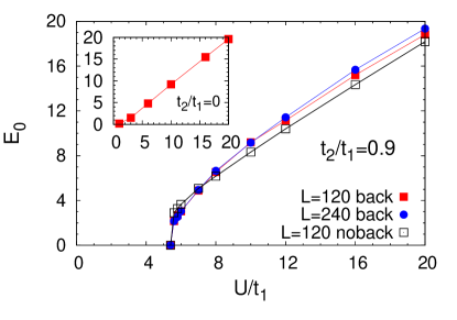
Figure 9: (Color online) Charge gap $E_{q}$ for $q\to 0$ for the 1D Hubbard model with $t_{2}/t_{1}=0.9$, on $L=120$ and $L=240$ lattices. Results without backflow correlations for the $L=120$ case are shown for comparison. Inset: charge gap for the 1D Hubbard model with $t_{2}=0$ on a $L=120$ lattice size. Axis labels are the same of the main plot.

VI Conclusions

The search for high-quality variational descriptions of the ground-state properties of correlated and frustrated electron systems is a long-standing issue. The problem lies in the correct description of emergent energy scales of order $t^{2}/U$, which are responsible both for the generation of antiferromagnetic correlations and spin-liquid behaviors of frustrated systems, as well as for incipient and real superconducting state formation.

The description of “dynamical” energy scales, viz of energy scales which are not explicitly present in the original Hamiltonian but are generated by dynamical processes (e.g., the super-exchange $J=4t^{2}/U$), is a challenge for both variational approaches and, more generally, for numerical simulations. It can be circumvented in the limit of large interactions, i.e., $U\gg t$, by using the $S$-matrix expansion outlined in Sec. III. One can then transform the Hubbard model into the $t{-}J$ model, for which there is no need to generate the antiferromagnetic energy scale, since it is already present explicitly in the model.

The $t{-}J$ model approach has played a key role in developing the RVB approach to high-temperature superconductivity. Within this framework, it is however not possible to study and correctly describe the Mott-Hubbard transition. With the backflow corrections, investigated in detail in the present study, it is instead now possible to describe, with a high degree of accuracy, the dynamical energy-scales of the Hubbard model both in the large- and the intermediate-$U$ region. We hence believe that substantial progress has been made towards the solution of a long-standing issue, namely the correct description of emergent energy scales in correlated and frustrated electron systems.

L.F.T. and C.G. acknowledge the support of the German Science Foundation through the Transregio 49.

Appendix A Jastrow factors and charge gap

As discussed in Sec. V, the insulating or metallic nature of the ground state of the Hubbard model can be determined by looking at the static structure factor $N(q)=\langle n_{-q}n_{q}\rangle$. Indeed, the behavior of this quantity for $q\to 0$ is related to the presence of a gap in the charge excitations of the system by Eq. (16). The insulating phase is characterized by $N(q)\sim q^{2}$ for $q\to 0$, while in the metallic phase $N(q)\sim q$.

A relation between the static structure factor and the Jastrow factor ${\cal J}=\exp(-1/2\sum_{q}v_{q}n_{q}n_{-q})$ has been derived in the context of liquid Helium by Reatto and Chester, reatto using a Gaussian approximation for the probability density associated to the uncorrelated ground state wave function $|\textrm{MF}\rangle$. We have that:

$$N(q)=\frac{N^{0}(q)}{1+2v_{q}N^{0}(q)},$$ (17)

where $N^{0}(q)$ is the static structure factor for the uncorrelated wave function $|\textrm{MF}\rangle$. This relation is rigorously valid in the weak-coupling regime; nevertheless, a similar behavior is found in the (strong-coupling) 1D insulating phase. capello2 The optimization of $v_{i,j}$ for every distance $|i-j|$, will lead, in $q$-space, to $v_{q}\sim 1/q$ for the metallic phase (in any dimension) and to $v_{q}\sim 1/q^{2}$ (in 1D) and $v_{q}\sim\log(q)/q^{2}$ (in 2D), see Fig. 4. Since $N^{0}(q)\sim\textrm{const}$ for $|\textrm{MF}\rangle=|\textrm{BCS}\rangle$ and $v_{q}$ diverges for $q\to 0$, the condition $2v_{q}N^{0}(q)\gg 1$ holds in the limit $q\to 0$ and one obtains

$$N(q)\sim\frac{1}{v_{q}}.$$ (18)

Therefore, the small-$q$ behavior of the structure factor reflects the small-$q$ behavior of the Jastrow factor. In the 2D insulating phase, although $v_{q}\sim\log(q)/q^{2}$ is found, the static structure factor shows a quadratic behavior, i.e., $N(q)\sim q^{2}$, highlighting the fact that corrections to Eq. (17) are present in the 2D Mott phase.

Appendix B Derivation of the single-particle charge gap

Given the ansatz for the excited state of Eq. (15), where $n_{q}=1/\sqrt{L}\sum_{r,\sigma}\textrm{e}^{iqr}n_{r,\sigma}$ is the Fourier-transformed particle density, the variational estimator of the excitation energy is then given by

$$E_{q}=\frac{\langle\Psi_{q}|({\cal H}-E_{0})|\Psi_{q}\rangle}{\langle\Psi_{q}|\Psi_{q}\rangle} = \frac{\langle\Psi|n_{-q}[{\cal H},n_{q}]|\Psi\rangle}{\langle\Psi_{q}|\Psi_{q}\rangle}$$

$$= \frac{\langle\Psi|[n_{-q}{\cal H}],n_{q}|\Psi\rangle}{\langle\Psi_{q}|\Psi_{q}\rangle},$$

where ${\cal H}$ is the Hamiltonian of Eq. (1). The sum of both commutators $(n_{-q}{\cal H}n_{q}-n_{-q}n_{q}{\cal H})+(n_{-q}{\cal H}n_{q}-{\cal H}n_{-q}n_{q})$ is equivalent to the double commutator

$$[n_{-q},[{\cal H},n_{q}]]=n_{-q}({\cal H}n_{q}-n_{q}{\cal H})-({\cal H}n_{q}-n_{q}{\cal H})n_{-q}$$ (20)

due to the inversion symmetry $q\leftrightarrow-q$. Therefore, the excitation energy is given by

$$E_{q}=\frac{1}{2}\frac{\langle\Psi|[n_{-q},[{\cal H},n_{q}]]|\Psi\rangle}{N_{q}},$$ (21)

where $N(q)=\langle\Psi|n_{-q}n_{q}|\Psi\rangle$ is the static structure factor for the ground state. The double commutator $[n_{-q},[{\cal H},n_{q}]]$ can be straightforwardly evaluated and involves the kinetic term only, since the potential term of the Hamiltonian contains density-density interactions that commute with $n_{q}$:

$$[n_{-q},[{\cal H},n_{q}]]=\frac{1}{L}\sum_{k,\sigma}(\epsilon_{k+q}+\epsilon_{k-q}-2\epsilon_{k})c^{\dagger}_{k,\sigma}c^{\phantom{\dagger}}_{k,\sigma}.$$ (22)

Therefore, in the limit of $q\to 0$, $E_{q}$ can be written as:

$$E_{q}=-\frac{1}{2\textrm{d}}\left(\lim_{q\to 0}\frac{|q|^{2}}{N(q)}\right)\left((\Delta r_{1})^{2}{\cal K}_{1}+(\Delta r_{2})^{2}{\cal K}_{2}\right)\,,$$ (23)

where d is the dimensionality, ${\cal K}_{1}$ and ${\cal K}_{2}$ are the nearest- and the next-nearest-neighbor kinetic energy per site, while $\Delta r_{1}$ and $\Delta r_{2}$ are the distances between nearest- and next-nearest-neighbors on the lattice (e.g., $\Delta r_{1}=1$ and $\Delta r_{2}=2$ or $\sqrt{2}$ on the 1D or 2D square lattice).

References

- (1) R.P. Feynman and M. Cohen, Phys. Rev. 102, 1189 (1956).
- (2) Y. Kwon, D.M. Ceperley, and R.M. Martin, Phys. Rev. B48, 12037 (1993); Phys. Rev. B58, 6800 (1998).
- (3) M. Holzmann, D.M. Ceperley, C. Pierleoni, and K. Esler, Phys. Rev. E68, 046707 (2003).
- (4) N.D. Drummond, P. López Ríos, A. Ma, J.R. Trail, G.G. Spink, M.D. Towler, and R.J. Needs, J. Chem. Phys. 124, 224104 (2006); P. López Ríos, A. Ma, N.D. Drummond, M.D. Towler, and R.J. Needs, Phys. Rev. E74, 066701 (2006).
- (5) L.F. Tocchio, F. Becca, A. Parola, and S. Sorella, Phys. Rev. B78, 041101(R) (2008); see also, F. Becca, L.F. Tocchio, and S. Sorella, J. Phys.: Conf. Ser. 145, 012016 (2009).
- (6) L.F. Tocchio, A. Parola, C. Gros, and F. Becca, Phys. Rev. B80, 064419 (2009).
- (7) L.F. Tocchio, F. Becca, and C. Gros, Phys. Rev. B81, 205109 (2010).
- (8) G. Carleo, S. Moroni, F. Becca, and S. Baroni, arXiv:1007.4260.
- (9) See for example, P. Fazekas, Lecture Notes on Electron Correlation and Magnetism, World Scientific (1999).
- (10) M. Capello, F. Becca, M. Fabrizio, S. Sorella, and E. Tosatti, Phys. Rev. Lett. 94, 026406 (2005).
- (11) H. Yokoyama and H. Shiba, J. Phys. Soc. Jpn. 59 3669, (1990).
- (12) A.H. MacDonald, S.M. Girvin, and D. Yoshioka, Phys. Rev. B37, 9753 (1988).
- (13) C. Gros, R. Joynt, and T.M. Rice, Phys. Rev. B36, 381 (1987).
- (14) D. Eichenberger and D. Baeriswyl, Phys. Rev. B76, 180504 (2007).
- (15) C. Gros, Phys. Rev. B38, 931(R) (1988).
- (16) F.C. Zhang, C. Gros, T.M. Rice, and H. Shiba, Supercond. Sci. Technol. 1, 36 (1988).
- (17) M. Capello, F. Becca, S. Yunoki, and S. Sorella, Phys. Rev. B73, 245116 (2006).
- (18) M. Capello, F. Becca, M. Fabrizio, and S. Sorella, Phys. Rev. Lett. 99, 056402 (2007).
- (19) S. Yunoki and S. Sorella, Phys. Rev. B74, 014408 (2006).
- (20) R. Chitra, S. Pati, H.R. Krishnamurty, D. Sen, and S. Ramasesha, Phys. Rev. B52, 6581 (1995).
- (21) D.F.B. ten Haaf, H.J.M. van Bemmel, J.M.J. van Leeuwen, W. van Saarloos, and D.M. Ceperley, Phys. Rev. B51, 13039 (1995).
- (22) R.P. Feynman, Phys. Rev. 94, 262 (1954).
- (23) S.M. Girvin, A.H. MacDonald, and P.M. Platzman, Phys. Rev. B33, 2481 (1986).
- (24) A.W. Overhauser, Phys. Rev. B3, 1888 (1971).
- (25) L. Reatto and G.V. Chester, Phys. Rev. 155, 88 (1967).