Ginzburg–Landau description of laminar-turbulent oblique band formation in transitional plane Couette flow

abstract : Plane Couette flow, the flow between two parallel planes moving in opposite directions, is an example of wall-bounded flow experiencing a transition to turbulence with an ordered coexistence of turbulent and laminar domains in some range of Reynolds numbers $[R_{\rm g},R_{\rm t}]$. When the aspect-ratio is sufficiently large, this coexistence occurs in the form of alternately turbulent and laminar oblique bands. As $R$ goes up trough the upper threshold $R_{\rm t}$, the bands disappear progressively to leave room to a uniform regime of featureless turbulence. This continuous transition is studied here by means of under-resolved numerical simulations understood as a modelling approach adapted to the long time, large aspect-ratio limit. The state of the system is quantitatively characterised using standard observables (turbulent fraction and turbulence intensity inside the bands). A pair of complex order parameters is defined for the pattern which is further analysed within a standard Ginzburg–Landau formalism. Coefficients of the model turn out to be comparable to those experimentally determined for cylindrical Couette flow.

1 Introduction

In their way to turbulence, wall-bounded shear flows display cohabiting turbulent and laminar regions. This striking phenomenon can even be statistically permanent and spatially organised, as for the flow between counter-rotating cylinders (cylindrical Couette flow, CCF) or counter-translating plates (plane Couette flow, PCF, Fig. 1, top-left). Cohabitation then takes the form of alternately turbulent and laminar oblique bands. This peculiar pattern was first discovered by Coles and Van Atta in CCF (barber-pole or spiral turbulence) [1], the corresponding domain in the control parameter space being next charted by Andereck et al. [2]. These experiments were restricted to the observation of a single spiral arm due to limited aspect-ratio (the ratio of the gap between the cylinders to the perimeter).

Later on, Prigent et al. [3] performed studies at larger aspect-ratios, which allowed them to observe several intertwined spiral arms and to show that the oblique bands in plane Couette flow (Fig. 1, bottom-left) were, qualitatively and quantitatively, the zero curvature limit of the spirals:

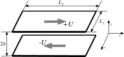
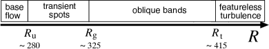
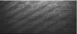
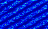
Figure 1: Top-left: Geometry of the plane Couette flow experiment, $2h$ is the gap, $L_{x}$ and $L_{z}$) the streamwise and spanwise dimensions, $+U$ and $-U$ the wall speeds. The Reynolds number is defined as $R=Uh/\nu$ where $\nu$ is the kinematic viscosity. Top-right: Experimental bifurcation diagram after Prigent [3, (a)]. Bottom: Picture of experimental banded turbulence in plane Couette flow apparatus with $L_{x}=770h$, $L_{z}=340h$ at $R=358$ (courtesy Prigent) and colour level representation of the perturbation energy averaged over $y$ in our under-resolved ChannelFlow simulations with periodic boundary conditions at $L_{x}=432$, $L_{z}=256$, $R=290$ and $t=18000$. The two pictures are at roughly the same scale and similar Reynolds numbers after correction for the transitional range $R$-shift due to numerical under-resolution[13].

Upon appropriate definition of a Reynolds number $R$ based on the nominal shear rate, (i) these patterns bifurcate continuously at similar values of a well-defined upper threshold $R_{\rm t}$ above which turbulence is featureless, (ii) the spirals/bands are observed upon decreasing $R$ down to comparable values of a lower stability threshold $R_{\rm g}$ below which laminar flow eventually prevails, and (iii) the streamwise and spanwise wavelengths are similar [4]. Figure 1 (top-right) recapitulates the experimental findings for PCF.

Direct numerical simulations (DNS) of the Navier–Stokes equations for PCF were performed by Barkley & Tuckerman [5] who could obtain the band patterns in fully resolved, elongated but narrow, tilted domains. Their choice of boundary conditions however precluded the occurrence of patterns with defects or orientation changes inside the flow. This was not the case of the DNS by Duguet et al. [6] who recovered the experimental findings of Prigent et al. in fully resolved very large aspect ratio domains. Similarly, the spiral regime was numerically obtained by Meseguer et al. [7] and Dong [8] in CCF and the oblique band pattern in plane channel flow by Tsukahara et al. [9].

Up to now, there is no clear physical explanation for the formation of the spirals/bands from the featureless turbulent regime when $R$ is decreased below $R_{\rm t}$ [10, b]. We however do have a consistent phenomenological description of the transition in CCF by Prigent et al. [3] in terms of two coupled Ginzburg–Landau equations with (strong) external noise added, introducing two complex amplitudes, one for each possible pattern orientation. Most of the coefficients introduced in these equations could be fitted against the experiments. In a similar vein, Barkley et al. [10] introduced the phase-averaged amplitude of the dominant Fourier mode of the turbulent mean flow modulation [5, b] as an order parameter for the PCF transition. The emergence of the bands was then identified from the position of the peak in the probability distribution function (PDF) of this order parameter, shifting from zero in the featureless regime to a nonzero value in the banded regime.

In the present article, we come back to the quantitative characterisation of the patterns in terms of order parameters. In contrast with [5, 10] we consider a configuration that does not freeze the orientation and allows for defective patterns. We keep the general noisy Ginzburg–Landau framework introduced in [3] for CCF and validate the approach in terms of amplitude equations at a quantitative level for PCF by means of numerical experiments. We take advantage of our previous work where the recourse to under-resolved DNS using Gibson’s public domain code ChannelFlow [11] was introduced [12]. In [13] we brought evidence that this procedure could be viewed as a consistent systematic modelling strategy permitting simulations in wide domains during long time lapses at moderate numerical load. We indeed showed that all qualitative aspects of the transitional range are preserved at the recommended resolution (Fig. 1, bottom-right) and that, in the (slightly better) numerical conditions chosen here, the resolution lowering amounts to a 15–20% downward shift of $[R_{\rm g},R_{\rm t}]$ from the experimental findings. This resolution reduction will allow us to accumulate statistics on moderate aspect ratio systems during very long times. We surmise that our results can be carried over to the realistic case of fully resolved simulations or experiments up to an appropriate adaptation of the Reynolds scale. We shall support this point of view briefly in §3.4.

We first recall the numerical procedure in §2.1, next we turn to the extraction of the turbulent fraction and the turbulence intensity (§2.2) and to the definition of order parameters able to include information about the spatial organisation, §2.3. Results are then analysed in the successive subsections of §3 devoted to the determination of the phenomenological parameters introduced by the Ginzburg–Landau formalism and accounting for the spanwise, streamwise and $R$ dependence of the pattern. Section 4 summarises our findings.

2 Simulations and data processing

2.1 Numerical implementation

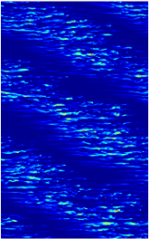
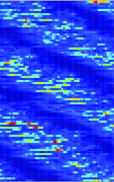
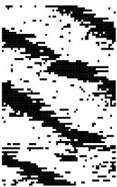
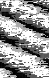
Figure 2: Top: $u_{x}^{2}$ in an $x,y$ plane, $L_{x}=128$ and in a $z,y$ plane, $L_{z}=180$. Bottom: From left to right, ${\bf u}^{2}$ in the $y=-y_{\rm m}$ plane, coarse-grained ${\bf u}^{2}$ in the $y<0$ domain, resulting B/W discrimination, and W/G/B discrimination (see text). $L_{x}\times L_{z}=128\times 180$, $R=315$.

The geometry of the experiment is described in Fig. 1 top-left. The Navier–Stokes equations are written in a reference frame where $x$, $y$, $z$ are the streamwise, wall-normal, and spanwise directions respectively. Velocities are made dimensionless with $U$ the absolute value of the speed at the boundaries $y=\pm h$. Lengths are rescaled by $h$ and time by $h/U$. The main control parameter is the Reynolds number $R=Uh/\nu$, where $\nu$ is the kinematic viscosity but the flow regime also depends on the aspect ratios defined as $\Gamma_{x,z}=L_{x,z}/2h$, where $L_{x,z}$ are the lateral streamwise and spanwise dimensions. In the numerics, $h=1$ and the aspect ratios are $\Gamma_{x,z}=L_{x,z}/2$. The base flow is independent of $R\,$: ${\bf v}_{\rm b}=y\,{\bf e}_{x}$. Written for the perturbation to the base flow ${\bf u}={\bf v}-{\bf v}_{\rm b}$, the Navier–Stokes equations read:

$$\partial_{t}u_{i}+\partial_{j}(u_{i}u_{j}) + y\partial_{x}u_{i}+u_{y}\delta_{i,x}$$

$$= \mbox{}-\partial_{i}p+R^{-1}\partial^{2}_{jj}u_{i}\,,$$

$$\partial_{j}u_{j} = 0\,,$$

with no slip boundary conditions at the plates, $u_{i}(y=\pm 1)=0$, and periodic boundary conditions at distances $L_{x}$ and $L_{z}$ in the streamwise and spanwise directions, respectively.

ChannelFlow [11] implements the Navier–Stokes equations using a standard pseudo-spectral scheme with Fourier transforms involving $(N_{x},N_{z})$ de-aliased modes in the streamwise and spanwise directions and $N_{y}$ Chebyshev polynomials in the wall-normal direction. As discussed in [13], our numerical simulations are deliberately under-resolved: we use $N_{y}=15$, and $N_{x,z}/L_{x,z}=8/3$, which preserves all the qualitative features of the flow at a semi-quantitative level, just shifting the bifurcation thresholds down to $R_{\rm g}=275\pm 5$ and $R_{\rm t}=345\pm 5$, to be compared with experimental or fully resolved numerical values, $R_{\rm g}\simeq 325$ and $R_{\rm t}\simeq 415$ [3, 6].

In PCF, Prigent et al. experimentally found oblique turbulent bands with streamwise period $\lambda_{x}\simeq 110$ and variable spanwise period $\lambda_{z}$ from $85$ around $R_{\rm g}$ to $45$ close to $R_{\rm t}$. The sizes of our numerical domains range from $L_{z}=24$ to $192$ and from $L_{x}=80$ to $170$. Our domains hence remain rather small since they can contain one to three such spanwise wavelengths but they are much larger than the minimal flow unit [14] of size $\ell_{x}\approx 6$ and $\ell_{z}\approx 4$, below which turbulence cannot self-sustain. They are also much longer in the streamwise direction than the tilted domains considered by Barkley et al. [5, 10] but remain smaller than the largest domains considered by Duguet et al. [6] or in our preliminary studies [13] which went up to $L_{x}=800$ and $L_{z}=356$ but at a much lower resolution, or the latest experiments by Prigent et al. with $L_{x}=770$ and $L_{z}=340$ [3].

2.2 Local averaging and related quantities

The square of the perturbation velocity ${\bf u}^{2}$ is a good indicator of the local state of the flow. Figure 2 (top) displays colour level representations of that quantity in typical wall-normal planes, streamwise $(x,y)$ with height 2 and length $L_{x}=128$, and spanwise $(z,y)$ with height 2 and width $L_{z}=180$, for $R=315$. The pattern seen from above in the $(x,z)$ plane at a given wall-normal coordinate $y=-0.57=-y_{\rm m}$ is displayed in Fig. 2 (bottom, left), the other panels represent the same image after additional post-treatment to be discussed below. The value $y_{\rm m}=0.57$ roughly corresponds to the place where ${\bf u}^{2}$ is statistically the largest in the range of Reynolds numbers of interest (see Fig. 5 in [13]).

The simplified representations shown in the centre and right panels of Fig. 2 rest on the coarse-graining of the ${\bf u}^{2}$ field introduced in [12]. This procedure directly stems from the general organisation of the flow in the band regime already identified in previous studies [1, 5] and clearly visible in the side and front views of the flow in Fig. 2 (top). These pictures suggest to average over the upper layer of the flow ($y>0$) and its lower layer ($y<0$) separately. Typical experimental observations [3, 2, 15], film and pictures, yield an information integrated over the whole gap, which motivates us to compute comparable quantities. As shown in Fig. 3, the computational domain is divided in small stacked boxes of size $l_{x}\times l_{y}\times l_{z}=2\times 1\times 2$. This size is slightly smaller than (but related to) that of the minimal flow unit. The width $l_{z}=2$ approximately corresponds to the spanwise size of a turbulent streak. By contrast, $l_{x}=2$ is much smaller than the typical length of a turbulent streak, $\tilde{l}\simeq 40$, so that the turbulent intensity variations along a streak can be captured. Quantity ${\bf u}^{2}$, henceforth called ‘energy’ by a small abuse of language, is then averaged in each of these cells and a threshold $c$ is chosen according to which it is laminar or turbulent. The turbulent fraction $f$ is then the proportion of turbulent cells, and the turbulent energy $e_{\rm t}$ is the energy conditionally averaged in space over the turbulent zone. Conditional averaging of any field can easily be performed in the same way. The reduction procedure is expected to depend on the value of $c$. As seen in Fig. 4 which displays the profile of the coarse-grained energy through the band pattern, the locally turbulent flow has typical energy higher than 0.1 and locally laminar flow less than 0.05. The computation of the time-averaged turbulent fraction $F$ and the time-averaged turbulent energy $E_{\rm t}$ for values of $c$ ranging from $0.005$ to $0.13$ did not pointed to an optimal value for $c$, as expected from a flow displaying a smooth modulation of turbulence, and $c=0.025$ was eventually chosen with little consequence on the quantitative information drawn from the procedure.

A typical example of this thresholding is given in Fig. 2, bottom line: from a realisation of the flow at $y=-y_{\rm m}$ (left) we compute the coarse-grained energy for $y<0$ (centre-left) and apply the criterion to obtain a black-and-white (B=laminar, W=turbulent) representation of the flow, still for $y<0$ (centre-right).

Figure 3: Sketch of the averaging boxes from the side and from above.

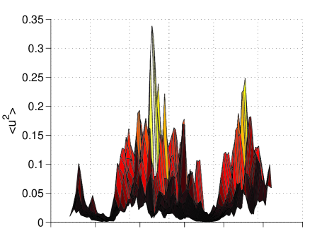
Figure 4: Coarse-grained $u^{2}$-profile projected along the direction of the turbulent band ($L_{x}\times L_{z}=128\times 64$, $R=315$, $y<0$).

Distinguishing the $y>0$ layer from the $y<0$ layers allows a refined representation of the flow as shown in the bottom-right panel of Fig. 2 which displays the turbulent and laminar areas using a black/gray/white code: ‘black’ represents laminar cells of top of each other, ‘white’ turbulent cells on top of each other, ‘light grey’ $y>0$ turbulent cells on top of $y<0$ laminar cells, and ‘dark grey’ $y<0$ turbulent cells of top of $y>0$ laminar cells [12]. As already seen in the top panels, the streamwise direction going from left to right, turbulence is to the right of the band for $y>0$ and to its left for $y<0$, in agreement with previous findings [1, 5]. This fact could be used to compute properties at the edge of the bands, for instance velocity or energy profiles. A quantitative comparison to results of Barkley and Tuckerman [5, b] has not been attempted since the differences in geometry and resolution shift the Reynolds number correspondence.

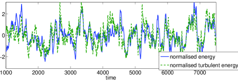
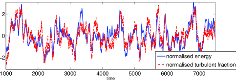
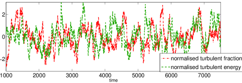
Figure 5: Time series of the normalised average energy $\bar{e}$, turbulent energy $\bar{e}_{\rm t}$ and the turbulent fraction $\bar{f}$ in a typical numerical experiment for $L_{x}\times L_{z}=110\times 48$ and $R=315$.

The procedure has been implemented on-line to allow the computation of time series of the turbulent quantities. Since these quantities fluctuate, we compute their time-averages $E$, $E_{\rm t}$, and $F$ as

$$E=\frac{1}{T}\int_{T_{0}}^{T_{0}+T}e(t)\,{\rm d}t\,,$$

where $T_{0}$ is introduced to take into account the transient necessary for the flow to reach its permanent regime, and $T$ is taken sufficiently large (typically, over $5000$) to keep the relative fluctuations of $E(T)$ within $0.5\,$%. The cut-off $c$ being appropriately chosen, the energy content of the laminar part is negligible so that we have $e\simeq f\times e_{\rm t}$, which means that the average energy of the flow is positively correlated to the changes of turbulence intensity in the bands measured by $e_{t}$, as well as to the fractional area $f$ occupied by the bands. On the other hand, quantities $e_{t}$ and $f$ do not show much correlation. This can be seen in figure 5 in which normalised quantities, $\bar{e}=(e-E)/(\langle e^{2}\rangle-E^{2})^{1/2}$, etc., are displayed. Computation of the correlation of $\bar{e}$ and $\bar{f}$, as well as $\bar{e}$ and $\bar{e}_{t}$ yields $0.5\pm 0.1$, on average over all experiments, whereas $\bar{e}_{t}$ and $\bar{f}$ are not correlated, yielding $0\pm 0.1$. Owing to small relative fluctuations, the relation $e\simeq f\times e_{\rm t}$ implies a similar relation, $E\simeq F\times E_{\rm t}$, for the averaged quantities.

It turns out that $e(t)$, $e_{\rm t}(t)$, and $f(t)$ are little affected by the orientation fluctuations: even when the pattern presents defects, the surface occupied by turbulence and the turbulence intensity in the bands remains essentially unchanged. This allows us to perform averaging regardless of the orientation, but $E$, $E_{t}$, and $F$ remain sensitive to the value of the bands’ wavelength imposed by the periodic boundary conditions fixing the in-plane dimensions $L_{x,z}$, as discussed below.

2.3 Order parameter

2.3.1 Conceptual framework and operational definitions

In the theory of phase transitions, an order parameter is an observable which, at the thermodynamic limit (permanent state at infinite size), is zero in the non-bifurcated state, here the featureless turbulent regime, and non-zero in the bifurcated state, here measuring the amount of coexisting laminar and turbulent domains. The turbulent fraction $F$ (introduced in [15] at a time when the spatially organised character of the banded regime was not yet recognised) or rather the laminar fraction $1-F$, partially fulfils this condition but remains of limited value since it does not account for the space periodicity of the pattern explicitly, which is what we want to overcome, inspired by previous work [3, 10]. In pattern-forming systems, the bifurcation is generally characterised by the amplitude of the relevant bifurcating mode and, especially in extended systems, by the amplitudes of the modes entering the Fourier decomposition of the structure that develops from the instability mechanism. When fitting the pattern-forming problem into the phase transition formalism, these amplitudes are the natural order parameters.

Figure 6

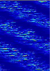
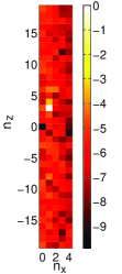
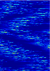
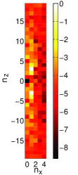
Figure 6: Color plots of patterns and natural logarithm of the corresponding spectra averaged over $y$ as explained in the text for a well-formed pattern (left) and for a pattern with defects (right). In the spectra, $\hat{u}_{x}(0,y,0)$ is set to zero, which yields a black dot in the spectra; normalisation by the maximum value makes its position appear the peak as a white dot. $L_{x}\times L_{z}=128\times 180$, $R=315$.

illustrates the result of a Fourier analysis of patterns with three bands fitting a domain of size $L_{x}\times L_{z}=128\times 180$. Symmetries in the spectrum allow us to consider wave numbers such that $0\leq n_{x}\leq N_{x}/2$, $-N_{z}/2+1\leq n_{z}\leq N_{z}/2$. The figure displays $(x,z)$-plots of ${\bf u}^{2}$ at $y=-y_{\rm m}$ (left) and corresponding spectra averaged over the wall-normal direction (right). The top panels correspond to an ideally formed pattern and the bottom panels to a defective one. For both flows, the wave numbers corresponding to the peak are $n_{x}=1$ and $|n_{z}|=3$. The spectra are zoomed on the smallest wave numbers so that modulations at the scale of the streaks are outside the reframed graphs. When the pattern is well formed, a single mode corresponding to the fundamental of the modulation clearly emerges, about two orders of magnitude larger than the other modes. These background modes account for small irregularities at a given time and not to steady anharmonic corrections to a basically sinusoidal profile: the average ratios $m_{n_{z}\neq 3}/m_{n_{z}=3}$ are at most $0.1$ and the harmonics have no definite phase relation with the fundamental, corroborating the observation by Barkley and Tuckerman that the modulation is quasi-sinusoidal [5, b]. In the defective case (figure 6, bottom), two peaks emerge, corresponding to the two orientations. Their amplitude is smaller, and other harmonics have non negligible amplitudes, accounting for the spatial modulations of the pattern. Envelopes can be defined, one for each orientation, obtained by standard demodulation.

The picture shown corresponds to a case with three bands, showing that there is enough room for a grain boundary. For smaller systems with one or two bands, defects correspond to the coexistence of laminar and turbulent regions without conspicuous organisation. In fact, the pattern can be observed only when the domain is above some minimal size $L_{x,z}^{\rm{min}}$. Our simulations suggest $L_{z}^{\rm{min}}\sim 24$ and $L_{x}^{\rm{min}}\sim 70$ (a precise determination of the minimal size is still under study). This is much smaller than in experiments because periodic boundary conditions tend to stabilise the pattern: only a tendency to form oblique turbulent patches was observed in laboratory experiments with $L_{x}\times L_{z}=280\times 72$ [15], where the ideal simple shear flow was achieved with sufficient accuracy only in the centre of the set-up due to lateral boundary effects.

Following Prigent et al [3, c], both orientations being equivalent, we expect that the pattern can be characterised by two complex quantities $A_{\pm}$:

$$u_{x}=\sum_{\pm}A_{\pm}\left(\tilde{x},\tilde{z},\tilde{t}\,\right)\exp i(k_{x}^{\rm c}x\pm k_{z}^{\rm c}z)+{\rm c.c.}\,,$$ (1)

where $A_{\pm}\in\mathbb{C}$ describe slow modulations at scales much larger than $\lambda_{x,z}^{\rm c}=2\pi/k_{x,z}^{\rm c}$, the ‘optimal’ streamwise and spanwise wavelengths. Variables ${\tilde{x}}$ and ${\tilde{z}}$ denote the corresponding space coordinates. Despite the highly fluctuating nature of the turbulent flow, the pattern being time-independent, there is just a possible slow evolution at an effective time $\tilde{t}$ linked to wavelength selection and defect dynamics. The modulus of $A_{\pm}$ gives the amplitude of the turbulent intensity modulation, and the phase fixes the absolute position of the pattern in the domain.

Near the threshold $R_{\rm t}$, introducing $\epsilon=(R_{\rm t}-R)/R_{\rm t}$, $A_{\pm}$ are guessed to fulfil Ginzburg–Landau–Langevin equations in the form [3]:

$$\tau_{0}\partial_{\tilde{t}}A_{\pm} = (\epsilon+\xi_{x}^{2}\partial_{\tilde{x}\tilde{x}}^{2}+\xi_{z}^{2}\partial_{\tilde{z}\tilde{z}}^{2})A_{\pm}$$ (2)

$$\quad\mbox{}-g_{1}|A_{\pm}|^{2}A_{\pm}-g_{2}|A_{\mp}|^{2}A_{\pm}+\alpha\zeta_{\pm}$$

where the $\alpha\zeta_{\pm}$ are additive noise terms expressing the local fluctuations caused by intense small scale turbulence, $\alpha$ being the strength of the physical noise. Though this noise is both more intense than thermal fluctuations (see [16] and references therein) and much more correlated since the featureless turbulent state is not without structure [18], terms $\zeta_{\pm}$ are tacitly taken as independent normalised delta-correlated Gaussian white noise processes ($\langle\zeta_{\pm}(t)\zeta_{\pm}(t^{\prime})\rangle=\delta(t-t^{\prime})$).

Periodic boundary conditions determine accessible wavelengths in a given domain: $\lambda_{x,z}=L_{x,z}/n_{x,z}$, where the integers $n_{x,z}$ are the wave numbers. In the computational domains considered here, with $L_{x,z}$ not so large, it turns out that states with $n_{x}=1$ or $2$ and $n_{z}=\pm 1$ up to $n_{z}=\pm 3$ can be observed, depending on the precise value of $L_{x}$ and $L_{z}$. When the wavenumbers are small enough, the partial differential model (2) can be reduced to a set of ordinary differential equations for scalar complex amplitudes, and when there is no wavelength competition but only an orientation competition playing with the $\pm$, just by two amplitudes $A_{\pm,n_{x},n_{z}}$ corresponding to a specific pair of wavenumbers ($n_{x},\pm n_{z}$). These amplitudes are then governed by:

$$\tau_{0}\partial_{\tilde{t}}A_{\pm,n_{x},n_{z}} = \tilde{\epsilon}_{n_{x},n_{z}}A_{\pm,n_{x},n_{z}}$$ (3)

$$\mbox{}-\left(g_{1}|A_{\pm,n_{x},n_{z}}|^{2}+g_{2}|A_{\mp,n_{x},n_{z}}|^{2}\right)A_{\pm,n_{x},n_{z}}+\alpha\zeta_{\pm}$$

with $\tilde{\epsilon}_{n_{x},n_{z}}=\epsilon-\xi_{x}^{2}\delta k_{x}^{2}-\xi_{z}^{2}\delta k_{z}^{2}$, $\delta k_{x,z}=k_{x,z}-k_{x,z}^{\rm c}$, and $k_{x,z}=2\pi n_{x,z}/L_{x,z}$, so that the dependence of the pattern on the value of the wavevectors can be studied by changing the size of the domain.

When a single wavelength and a single orientation are selected, a single complex amplitude can serve to characterise the corresponding pattern. This was precisely the case considered by Barkley & Tuckerman [5] who defined the order parameter from a single Fourier amplitude by sampling its probability distribution function (PDF) and averaging over its phase [10]. So doing, they were able to detect the bifurcation to the band regime from the change in the PDF as $R_{\rm t}$ was crossed. In our simulations a single orientation is selected only deep enough in the band regime, i.e. sufficiently below $R_{\rm t}$ but above $R_{\rm g}$. The pattern is then well installed and its orientation remains fixed but its lateral position in the domain can fluctuate, which strictly corresponds to the phase fluctuations alluded to above. When this is the case, symmetry considerations underlying (3) imply that the phase is dynamically neutral, hence constant in a deterministic context, while it is expected to evolve as a random walk in a noisy context [10]. Figure 7 shows that this is indeed the case.

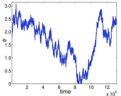
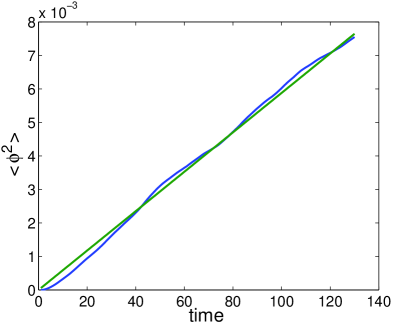
Figure 7: Top: Variation with time of the phase of the main Fourier component of $\hat{u}_{x}$ for $L_{x}=110$, $L_{z}=48$, $R=290$. Bottom: growth of the variance of the ensemble-averaged fluctuations as a function of time ($T_{\rm e}=130$, $N_{\rm e}=1000$), with linear fit.

The top panel illustrates the variations of the phase of the Fourier amplitude $\hat{u}_{x}$ of the streamwise velocity component at $y=-y_{\rm m}$ for $R=290$ in a domain of size $L_{x}\times L_{z}=110\times 48$. The expected property is illustrated in the bottom panel which displays the linear growth of the variance of the phase fluctuations as a function of time after appropriate ensemble averaging: From the initial time series we define an ensemble of $N_{\rm e}$ successive sub-series of duration $T_{\rm e}$ as:

$$\phi_{i}(t)=\phi(t+(i-1)T_{\rm e})-\phi\left((i-1)T_{\rm e}\right)\,,\quad t\in\left[0,T_{\rm e}\right]$$

for $i=1\dots N_{\rm e}$. We next define the ensemble average:

$$\langle\phi\rangle(t)=\frac{1}{N_{\rm e}}\sum_{i=1}^{N_{\rm e}}\phi_{i}(t)\,,\quad t\in\left[0,T_{\rm e}\right]\,.$$

which always remains of order $10^{-3}$, while the variance:

$$\sigma_{\phi}^{2}(t)=\frac{1}{N_{\rm e}}\sum_{i=1}^{N_{\rm e}}\left(\phi_{i}(t)-\langle\phi\rangle(t)\right)^{2}\,,\quad t\in\left[0,T_{\rm e}\right]$$

is indeed seen to grow linearly with time (Fig. 7).

When the wavelength and/or the orientation can fluctuate, as is now the case of interest, the practical definition of an order parameter is less straightforward since a single complex amplitude is not enough. Here, we forget about the information contained in the phase of the relevant complex amplitudes and focus on their modulus. We then define the instantaneous order parameter $m_{n_{x},n_{z}}(t)$ as the modulus at time $t$ of the fundamental Fourier mode $(n_{x},n_{z})$ accounting for the pattern as featured by the streamwise velocity field $u_{x}$ averaged along the wall-normal direction:

$$m_{n_{x},n_{z}}(t)=\left(\frac{1}{2}\int_{-1}^{1}|\hat{u}_{x}(n_{x},y,n_{z},t)|^{2}\,{\rm d}y\right)^{1/2}$$ (4)

but equivalent results are obtained from the other velocity components, with or without wall-normal averaging.

2.3.2 Typical experiments and the order-parameter time-averaging issue

Owing to the linear stability of the laminar flow, turbulence has to be triggered by finite amplitude disturbances. A typical experiment consists of creating a random initial condition and evolving it at a Reynolds number for which uniform turbulence is expected, here $R=450$ ($\gg R_{\rm t}\simeq 345$ at the resolution chosen in the present work). That state is next used as an initial condition for a simulation at the targeted value of $R$ for which the pattern of interest is expected, hence $R_{\rm g}<R<R_{\rm t}$. Such experiments were named quench in [15, 17]. Variations of turbulent quantities $e(t)$, $e_{\rm t}(t)$, $f(t)$ and of the order parameters $m(t)$ at the beginning of a typical experiment are shown in Fig. 8:

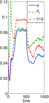
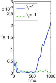
Figure 8: Time series of turbulent quantities (left) and $m$ (right) during the initial stage of a typical experiment. Here, for $L_{x}\times L_{z}=110\times 48$, $R$ is initially set at 450 and switched to 315 at $t=500$.

The stabilisation of the featureless regime at $R=450$ is clearly visible with $e\simeq e_{\rm t}$, $f/10\simeq 0.1$ (left), and $m\sim 0$ (right). The subsequent quench at $t=500$, $R=315$ is seen to produce some undershoot of $e$, $e_{\rm t}$ and $f$, while $m$ grows slowly, which corresponds to the formation of bands. After a short period of exponential growth, the order parameters saturate as shown in Fig. 9 for a series of 6 independent runs in the same conditions where a band is expected, pointing out the selection of the orientation, with one of the order parameters larger than the other by typically one to two orders of magnitude.

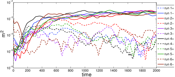
Figure 9: Time series of $m^{2}$ for six different runs at $R=315$, with $L_{x}\times L_{z}=128\times 48$, starting from uniform turbulence (time is reset upon quenching). $+$ and $-$ refer to $n_{z}=+1$ and $n_{z}=-1$. Mode $+1$ is selected in runs 2, 3, 4, and mode $-1$ in runs 1, 5, 6. (colour online)

The simulation is continued during at least $5000$ time units in order to ensure good convergence of the time averages $E$, $E_{t}$, $F$ and $M$. The same procedure is repeated for all the values of $L_{x}$, $L_{z}$, and $R$ considered, except in §3.4 where an adiabatic procedure is adopted to vary $R$.

Like the turbulent quantities $e$, $e_{\rm t}$ and $f$, order parameters $m_{n_{x},n_{z}}$ fluctuate in time but, since orientation changes are now of interest, care is required when computing their averages. Figure 10 displays a typical example of

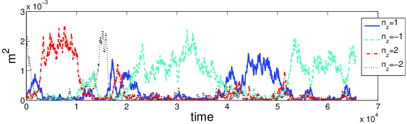
Figure 10: Time series of $m^{2}$ for $L_{x}\times L_{z}=128\times 84$ at $R=315$. Well-formed patterns with $n_{z}=+1$ appear for $t\in[43,51]$, $n_{z}=-1$ for $t\in[22,37]$ and $t>52$, $n_{z}=+2$ for $t\in[3,11]$, and $n_{z}=-2$ for $t\in[14,16]$. Defective patterns are obtained for $t\in[18,22]$ or $[38,43]$. (All times to be multiplied by $10^{3}$.)

long-lasting time series of $m^{2}$ for $L_{x}=128$, $L_{z}=84$, and $R=315$, which produces patterns with $n_{x}=1$ and $|n_{z}|=1$ and $2$, so that modes $n_{z}=\pm 1$ and $\pm 2$ dominate in turn. As long as the instantaneous state of the system is close to ideal, $m$ fluctuates around a specific mean value which depend only on $|n_{z}|$ as expected from symmetry considerations. Defects may appear and disappear, involving several modes with similar amplitudes. For the data in Fig. 10, $L_{z}=84$ lies in a range $L_{z}\in]80,96[$ where the competition between different values of $|n_{z}|$ is particularly intense (see below). When it is the case, a proper definition of order parameters implies conditional averaging over periods during which the pattern is well formed with the chosen value of $|n_{z}|$. For example, in Fig. 10, $|n_{z}|=1$ is present during about 3/4 of the time window and $|n_{z}|=2$ less than 1/4 of it. Since $m_{\pm 2}>m_{\pm 1}$ when the corresponding modes dominate the pattern, one gets $M_{2}>M_{1}$, but it would be meaningless to make a blend of the two and define a single order parameter for the system. A detailed study of this special case is deferred to [19].

However, outside cases of strong wavelength competition, a single value of $|n_{z}|$ is selected, which makes things somewhat easier and allows us to simplify the notation: $m_{n_{x},\pm n_{z}}\mapsto m_{\pm}$. An example is displayed in Fig. 11 for $L_{z}=32$ where only $|n_{z}|=1$ shows up.

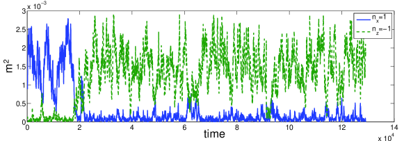
Figure 11: Time serie of $m^{2}(t)$ for $L_{x}\times L_{z}=110\times 32$, $R=330$

Averaging can then be performed from two-dimensional probability distribution functions (PDF) $\Pi_{\rm e}(m_{+},m_{-})$, where subscript ‘e’ means ‘empirical’.

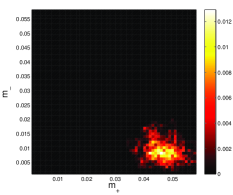
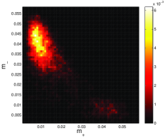
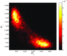
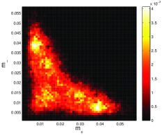
Figure 12: PDF of $m$ for $L_{x}\times L_{z}=110\times 32$, $R=290$ (left), $R=330$ (centre-left), $R=330$, symmetrised (centre-right), $R=337$, symmetrised (right).

Far away from $R_{\rm t}$ the orientation does not fluctuates and the pattern remains without defects, which yields a one-hump PDF such as the one in Fig. 12 (left) for $R=290$, but closer to $R_{\rm t}$ the orientation fluctuates and defects are present. Two humps are then obtained as in Fig. 12 (centre-left) which derives from the time series for $R=330$ shown in Fig. 11. Due to the finite length of the time series, the PDF is not symmetrical with respect to the diagonal but since, for symmetry reasons, the two orientations should be present with the same weight, one may improve the statistics by constructing $\Pi_{\rm e,s}(m_{+},m_{-})=\frac{1}{2}\left(\Pi_{\rm e}(m_{+},m_{-})+\Pi_{\rm e}(m_{-},m_{+})\right)$, where the additional subscript ‘s’ means ‘symmetrised’, which is done in Fig. 12 (centre-right). Averages can then be extracted from the ‘symmetrised’ PDF, which works fine as long as the orientation fluctuates but neither the wave numbers $n_{x}$ nor $|n_{z}|$. We thus define:

$$M=2\int_{m^{\prime\prime}<m^{\prime}}m^{\prime}\Pi_{\rm e,s}(m^{\prime},m^{\prime\prime})\,{\rm d}m^{\prime}{\rm d}m^{\prime\prime}\,.$$

The right panel in Fig. 12 displays the (symmetrised) PDF for $R=337$, when re-entrant featureless turbulence intermittently bursts in, which manifests itself as a secondary hump close to the origin, see below §3.4, and especially the discussion related to Fig. 17.

3 Results

3.1 Theoretical expectations

The statistically steady states (permanent regimes) obtained in the DNS and characterised by the time-averaged empirical order parameters $m_{n_{x},n_{z}}$ defined through (4) can then be compared to the equilibrium states predicted by model (3), the deterministic part of which can be written as deriving from the potential:

$${\cal V} = -\mbox{$\frac{1}{2}$}\tilde{\epsilon}\left(|A_{+}|^{2}+|A_{-}|^{2}\right)+\mbox{$\frac{1}{4}$}g_{1}\left(|A_{+}|^{4}+|A_{-}|^{4}\right)$$ (5)

$$\mbox{}+\mbox{$\frac{1}{2}$}g_{2}|A_{+}|^{2}|A_{-}|^{2}\,,$$

where $\tilde{\epsilon}$ is a short hand notation for $\tilde{\epsilon}_{n_{x},n_{z}}$, computed from the values of $n_{x}$ and $\pm n_{z}$ relevant to the pattern of interest, again with a single pair of modes present in the system.

Assuming Gaussian noises of strength $\alpha$, the theoretical expression of the PDF reads [20]:

$$\Pi_{\rm t}(m_{+},m_{-})=Z^{-1}\,m_{+}m_{-}\exp(-2{\cal V}/\alpha^{2})\,,$$

where subscript ‘t’ means ‘theoretic’ and

$$Z=\int_{0}^{\infty}\int_{0}^{\infty}m_{+}m_{-}\exp(-2{\cal V}/\alpha^{2})\,{\rm d}m_{+}{\rm d}m_{-}$$

is a normalisation factor called the partition function in statistical physics. For values of $\tilde{\epsilon}$ that are not too small, the most probable values $m_{\pm}^{0}$ corresponding to the maxima of $\Pi_{\rm t}$ give a good estimate of expected mean values $\langle m_{\pm}\rangle$ (mean-field approximation). They are given by the solutions to:

$$0=-\tilde{\epsilon}m_{\pm}^{2}+g_{1}m_{\pm}^{4}+g_{2}m_{\pm}^{2}m_{\mp}^{2}-\alpha^{2}/2\,.$$

At lowest non-trivial order in $\alpha^{2}$, we have:

$$m^{0}_{\pm}\propto\frac{\alpha}{|\tilde{\epsilon}|}\,,$$ (6)

which corresponds to the trivial solution of the deterministic problem, just shifted by the effects of noise. The non-trivial solutions read:

$$m^{0}_{+}=m^{0}_{-}=\sqrt{\tilde{\epsilon}/(g_{1}+g_{2})}$$ (7)

and

$$m^{0}_{\pm}=\sqrt{\tilde{\epsilon}/g_{1}}\,,\quad m^{0}_{\mp}=\frac{\alpha}{\sqrt{2\tilde{\epsilon}(g_{2}-g_{1})/g_{1}}}$$ (8)

For $\tilde{\epsilon}<0$, solution (6) is stable and the other solutions do not exist. For $\tilde{\epsilon}>0$, solution (6) is unstable and the symmetric solution (7) is a saddle point since, in order to get a stripe pattern we assume $g_{2}>g_{1}$; otherwise a stable rhombic pattern would be obtained but is observed neither in the experiments nor the numerical simulations. This solution lies on the boundary of the attraction basins of solutions (8), which exist for $\tilde{\epsilon}>0$ and are stable. They represent the amplitude of the turbulence modulation for $R<R_{\rm t}$. The mean amplitude of the installed mode varies as $\sqrt{\tilde{\epsilon}}$ as is typical of a supercritical bifurcation. The other mode, expected to be zero in the deterministic case, is present with small amplitude due to noise. Noise is also responsible for a switch from the ‘$\pm$’ situation to the ‘$\mp$’ one when fluctuations make the system leave the well corresponding to an installed ‘$+$’ mode to reach the other one where the ‘$-$’ mode is installed and vice versa, going through the potential barrier at the saddle solution (7). The asymptotic expressions above agree with the values computed from the PDFs obtained by direct simulations of model (3) and will be plotted together with our results in Figures 19 and 21. When $\tilde{\epsilon}$ is very small, fluctuations around the most probable values have to be taken into account. The mean field approximation is no longer valid and a behaviour in the form $\langle m_{\pm}\rangle\propto|\tilde{\epsilon}|^{\beta}$ is expected, where $\beta$ is the critical exponent describing the variations of the order parameter with the control parameter in the theory of phase transitions. We shall restrict to the mean-field approximation as a first guess since the nature and extent of this specific regime, called critical in statistical physics, are not yet clearly characterised in the present case (see [16] and references therein for examples where fluctuations have thermal origin).

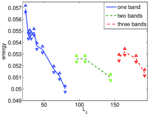
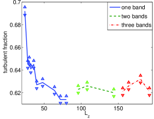
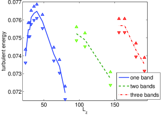
Figure 13: Perturbation energy $E$ (left), turbulent fraction $F$ (center) and turbulent energy $E_{t}$ (right) as functions of $L_{z}$ for $L_{x}=128$ and $R=315$.

The deterministic part of model (3) is invariant against phase changes of the complex amplitudes $A_{\pm}=m_{\pm}\exp(i\phi_{\pm})$, implying that the $\phi_{\pm}$ are dynamically neutral. They are indeed governed by:

$$\tau_{0}\partial_{\tilde{t}}\phi_{\pm}={\cal I}m\left[\exp(-i\phi_{\pm})\alpha\zeta_{\pm}\right]/m_{\pm}\,,$$ (9)

i.e. a stochastic process, the strength of which depends on the instantaneous value of $m_{\pm}$. In fact, the right hand side of (9) is another random Gaussian process $\tilde{\zeta}(t)\alpha/m(t)$ with zero mean and variance $\alpha^{2}\delta(t-t^{\prime})/(\langle m\rangle^{2}+\sigma_{m}^{2})$ where $\sigma_{m}^{2}$ is the variance of $m(t)$, which can be checked numerically using model (3). Results in Fig. 7 above can be quantitatively rendered by taking $\alpha/\tau_{0}=4\times 10^{-4}$.

Coherence lengths $\xi_{x}$ and $\xi_{z}$ in (3) control how strictly the wavevectors $k_{x}$ and $k_{z}$ are bound to their optimal values $k_{x}^{\rm c}$ and $k_{z}^{\rm c}$. The anisotropy of the base flow leads to expect different values for $\xi_{x}$ and $\xi_{z}$. For PCF, experimental data [3] suggests that $\lambda_{x}$ and therefore $k_{x}$ do not depend on the Reynolds number, whereas $\lambda_{z}$ decreases with $R$. Prigent et al. also report a decrease of the effective value of $\xi_{z}$ as $R$ is increased but the experiment did not give access to $\xi_{x}$. In the following, we determine most of coefficients in model (3) from the dependence of $E$, $E_{\rm t}$, $F$ and $M$ on $k_{z}$, $k_{x}$, by varying $L_{x}$, $L_{z}$ and $R$ using the quench protocol explained above. The dependence upon the Reynolds number analysed next is obtained from simulations in which $R$ is varied adiabatically.

3.2 Dependence on $k_{z}$

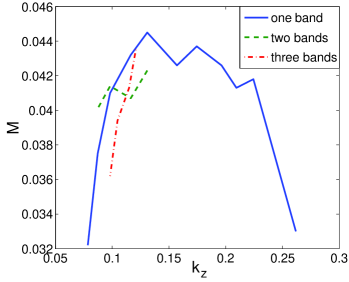
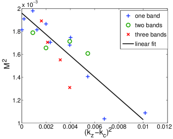
Figure 14: Order parameter squared $M$ as a function of $k_{z}$ (left) and of $(k_{z}-k_{z}^{\rm c})^{2}$ (right) for $L_{x}=128$ and $R=315$.

We fix $R=315$, in the middle of the range where bands are expected at the resolution that we consider [13], and $L_{x}=128$ so that a single streamwise period is obtained ($n_{x}=1$, $k_{x}=2\pi/L_{x}$). We take values of $L_{z}$ ranging from 24 to 192. Taking the number $|n_{z}|$ of spanwise periods into account, we have $k_{z}=2\pi|n_{z}|/L_{z}$. Figure 13 displays $E$, $E_{t}$, and $F$ as functions of $L_{z}$, showing that $|n_{z}|$ increases with $L_{z}$: one band for $24\leq L_{z}\leq 80$, two bands for $96\leq L_{z}\leq 144$ and three bands for $156\leq L_{z}\leq 192$. In these ranges, $|n_{z}|$ stays fixed during the simulation. In contrast, patterns with $|n_{z}|=1$ and $|n_{z}|=2$ alternate in time for $80<L_{z}<96$, here for $L_{z}=84$ (see figure 10) and $L_{z}=90$. This special case is studied more thoroughly in [19]. A similar competition between $|n_{z}|=2$ and $|n_{z}|=3$ is expected to occur for $144\lesssim L_{z}\lesssim 150$. Taken together, the results in Fig. 13 illustrate confinement effects when $L_{z}$ is small. Turbulence is featureless for $L_{z}<24$ and the turbulent fraction $F$ (central panel) rapidly decreases from 1 down to $\simeq 0.63$ which therefore represents some kind of optimum at $R=315$.

The results also suggest to check cases with $n_{z}>1$ against case $n_{z}=1$. Figure 14 (top) displays $M^{2}$ as a function of $k_{z}=2\pi n_{z}/L_{z}$ and $n_{z}=1$ as a full line. Data obtained with two and three bands are also shown as dashed and dash-dotted lines, respectively. For them no points at large wavevectors are obtained because the corresponding patterns are not stable enough to be observed. The parabolic shape expected from the theory (§3.1) is reasonably well reproduced by the data. The maximum is reached at $k_{z}^{\rm c}\simeq 0.16$, that is $\lambda_{z}^{\rm c}=2\pi/k_{z}^{\rm c}\simeq 39$, as determined from a fit against a parabola. The so-obtained value of $k_{z}^{\rm c}$ can next be used to determine $\xi_{z}^{2}$ from the slope of a linear fit of $M^{2}$ against $(k_{z}-k_{z}^{\rm c})^{2}$. The result is displayed in Figure 14 (bottom) where data corresponding to one band are shown with ‘$+$’ signs. From it one derives $\xi_{z}^{2}/g_{1}=0.1$. In turn, the constant term in the fit is a compound accounting for the dependence on $R$ and $k_{x}$, namely $(\epsilon-\xi_{x}^{2}\delta k_{x}^{2})/g_{1}=0.002$. Data for two and three bands, respectively shown with ‘$\circ$’ and ‘$\times$’ symbols, are seen to be consistent with these estimates. Here a single value of $R$ has been considered. In the CCF case, Prigent et al. found for $\xi_{z}^{2}/g_{1}$ values of the same order of magnitude, decreasing with $R$ from $0.5$ to $0.1$ [3, c].

3.3 Dependence on $k_{x}$

The dependence of the pattern’s characteristics on $k_{x}$ is studied for $R=315$, $L_{z}=48$, and $L_{x}\in[80,170]$. In this range, only $n_{x}=1$ is obtained, except for $L_{x}=170$ where $n_{x}=2$ can also be observed. Figure 15 shows that, as a function of $k_{x}$ (top), $M^{2}$ displays a maximum at $k_{x}^{\rm c}=0.058$, hence $\lambda_{x}^{\rm c}=110$, whereas fitting $M^{2}$ against $(k_{x}-k_{x}^{\rm c})^{2}$ (bottom) yields $\xi_{x}^{2}/g_{1}=2.7$. The same study at $R=330$ (closer to $R_{\rm t}=345$) gives $\lambda_{x}^{\rm c}=110$ and $\xi_{x}^{2}/g_{1}=3.9$, while at $R=290$ (closer to $R_{\rm g}=275$) we get $\lambda_{x}^{\rm c}=125$ and $\xi_{x}^{2}/g_{1}=2.2$, which is a rough estimate since the lack of symmetry in the exchange $\delta k_{x}\leftrightarrow-\delta k_{x}$ visible in the top panel of Fig. 15 has not been taken into account.

The variation of $\lambda_{x}^{\rm c}$ with $R$ that we obtain here is not observed in the the plane Couette flow experiments but remains compatible with the trend seen in CCF case [3, a]. Rather than to the role of rotation or curvature, this observation points to the role of streamwise periodic boundary conditions enforced by the cylindrical geometry or the numerical implementation.

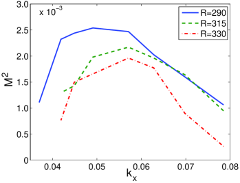
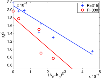
Figure 15: Order parameter squared $M^{2}$ as a function of $k_{x}$ (left) and of $(k_{x}-k_{x}^{\rm c})^{2}$ (right) for $L_{z}=48$ and $R=315$.

3.4 Dependence on $R$

Variations of $E$, $F$, $E_{\rm t}$, and $M$ against $R$ are studied using a different protocol. Two sizes are considered: $L_{x}\times L_{z}=128\times 64$ and $110\times 32$. From the study in previous sections, both domains are expected to fit one elementary band $\lambda_{x}\times\lambda_{z}$. The pattern should feel “at ease” in the first domain and more “spanwise-confined” in the second one. A first simulation at $R_{0}=315$ serves to prepare initial conditions for simulations at higher and lower Reynolds numbers by increasing or decreasing $R$ by steps $\Delta R=5$. The flow is integrated over $5000$ time units at each value of $R$ and the so-obtained state is used as an initial condition for the next value of $R$ in the range $[260,350]$. Additional values $R=333$, $336$, $337$, and $R=370$ and $390$ outside the interval are also considered. At given $R$ statistical results involve time integration over at least $1.5\times 10^{4}$ time units.

The main effect of increasing $R$ seems to be an expansion of the turbulent part of the band pattern as illustrated in Fig. 16. When $R$ is close enough to $R_{\rm t}$ the orientation of the pattern fluctuates: destroying a well-established ideal pattern, turbulence invades the laminar band, stays featureless for a while, before another pattern grows, which may or may not have the same orientation.

     

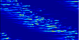
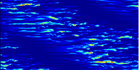
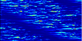
Figure 16: Colour plot of ${\bf u}^{2}$, from left to right: $R=280$, $R=300$ and $R=330$. $L_{x}\times L_{z}=128\times 64$.

Figure 17 displays a featureless turbulent episode for $L_{x}\times L_{z}=110\times 32$ and $R=335$, during which $m(t)$ stays close to $0$ (left panel), the turbulent fraction approaches one, indicating the decrease of the size of the laminar domain and commanding the variation of the total energy (central panel), while the intensity of turbulence inside the turbulent domain does not changes (right panel). Such events cannot be mistaken with the transient occurrence of a defect in the pattern since both $m_{+1}$ and $m_{-1}$ remain simultaneously close to zero for a relatively long period of time, which is characteristic of the featureless state.

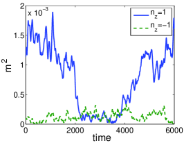
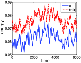
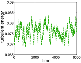
Figure 17: Time series of $m$ (left), $e$ and $f/10$ (center) and $e_{\rm t}$ (right) zoomed on the appearance and disappearance on an uniformly turbulent flow for $L_{x}\times L_{z}=110\times 32$ and $R=335$.

They are not observed for $R\leq 333$, and go from extremely rare at $R=335$ and $337$ to common at $R=340$, to the most common state at $R=345$ (though a trace of modulation persists).

Since it is a three-state jump process instead of a two-state one, this feature should be treated appropriately following the same procedure as for orientation fluctuations. However, it cannot be accounted for by the plain model (3) since empirical PDFs for $R=337$ (Fig. 12, right) and higher clearly present three maxima, one of which is close to the origin ($m_{+}\simeq 0\simeq m_{-}$). The phenomenon can however be treated within the same conceptual framework by assuming a slightly modified potential with an additional relative minimum at the origin separated by saddles from the main minima corresponding to the pattern installed in one or the other orientation, justified by the appearance of a third maximum in the PDFs. The splitting probability between the featureless regime and the pattern would then be controlled by the relative depths of the three wells [20], which could be studied by following the procedure for orientation fluctuations [19]. This complication has however not been explored further because the phenomenon is likely a size effect: In the upper transitional regime at large aspect-ratio, bands form out of scattered elongated regions where turbulence is depleted, see Fig. 18.

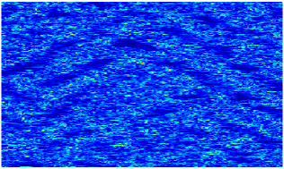
Figure 18: Snapshot of the numerical solution for $R=340$ at $t=20000$; same simulation conditions as in Fig. 1 (bottom-right), in particular $L_{x}=432$, $L_{z}=256$.

The computational domains considered here are just sufficient to contain a pattern cell of size $\lambda_{x}\times\lambda_{z}$. It is therefore not surprising that the spatiotemporal intermittence of laminar troughs comparable in size to that cell be turned into temporal intermittence of well-formed laminar bands recurrently destroyed by featureless turbulence. The improved modelling suggested above would transform the supercritical bifurcation into a slightly subcritical one, with associated coexistence of featureless and patterned states, as expected from system where a spatial and temporal cohabitation of different states is possible. This would explain the shape of the PDFs once noise is introduced as for the original model. The same explanation, if correct, would explain the presence of the ‘intermittent regime’ described, although not fully investigated, by Barkley & Tuckerman [5, 10] since turbulence modulations around $R_{\rm t}$ are also much longer than the width of the oblique computational domain they considered.

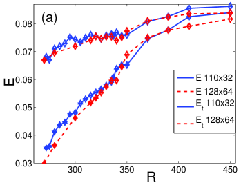
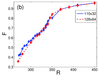
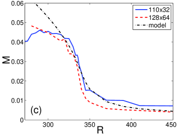
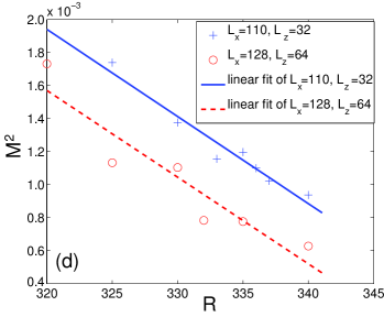
Figure 19: Variation with $R$ of the different averaged quantities for domains $L_{x}\times L_{z}=110\times 32$ (blue on line) and $128\times 64$ (red on line): (a) Perturbation energy $E$ (full line) and turbulent energy $E_{\rm t}$ (dashed line). (b) Turbulent fraction $F$. (c) Order parameter $M$ and corresponding values from the model (dash-dotted line, $g_{1}=55$, $g_{2}=250$, $\alpha=0.002$, $R_{\rm t}=355$). (d) Square of the order parameter $M^{2}$, observations ($\circ:128\times 64$ and $+:110\times 32$) and linear fits (lines).

Figure 19 displays the variations of the different observables of interest with $R$. The growth of the width of the turbulent domain illustrated in Fig. 17 is clearly reflected by the increase of $F$ with $R$ in Fig. 19 (b). Quantity $F$ varies roughly linearly with $R$ for $R<R_{\rm t}$, and with a much smaller slope above. This increase mostly explains the growth of the perturbation energy since the turbulent energy depends more weakly on $R$, with no singular behaviour visible at $R_{\rm t}$ (Fig. 19, a): the intensity of turbulence inside the turbulent domains does not seem sensitive to the global organisation in an oblique pattern. The slope discontinuity at $R_{\rm t}\simeq 350$ marking the bifurcation was used as a criterion in our previous study [13]. Values obtained for $E$, $E_{t}$, and $F$ are slightly different for the two sizes considered, which is related to lateral confinement effects already illustrated in Fig. 13 (left) for $R=315$.

In Figure 19 (c), it can be seen the order parameter $M$ departs from the expected classical $\tilde{\epsilon}^{1/2}$ behaviour and tends to saturate in the lowest part of the transitional range. For $L_{x}\times L_{z}=110\times 32$, it even decreases as $R$ is lowered further, which is again a confinement effect since, from the experiments [3] as well as from our earlier (less well resolved) numerical results [13], the spanwise wavelength $\lambda_{z}$ is expected to increase up to about $80$ as $R$ decreases: this implies a less optimal pattern and a weaker modulation for $L_{z}=32$, while for $L_{x}\times L_{z}=128\times 64$, with a more favourable $\lambda_{z}$, $M$ continues to increase as $R$ is lowered in agreement with the Ginzburg–Landau picture. In the upper part of the transitional range, $M$ decreases quickly as $R$ increases. The decay of the modulation corresponds to the increase of the width of the turbulent domain. Again in line with the Ginzburg–Landau interpretation, the variation of $M^{2}$ with $R$ (Fig. 19, d) appears to be linear with a slope $1/(g_{1}R_{\rm t})\simeq-5.3\times 10^{-5}$. Meanwhile, the extrapolation of $M^{2}$ to zero gives a value of $R_{\rm t}\approx 355$ or $348$ depending on whether one takes the data from case $L_{x}\times L_{z}=110\times 32$ or $128\times 64$, respectively. In contrast with what happens for $R\sim R_{\rm g}$, here the estimate with $L_{z}=32$ is likely the best one since experiments suggest $\lambda_{z}\simeq 37.5$ either by extrapolation for plane Couette flow or from measurements in the CCF [3]. Taking $R_{\rm t}\simeq 355$, we get $g_{1}\simeq 55$, which is consistent with Prigent’s value $g_{1}\sim 100$ in the CCF case. This value of $g_{1}$ further yields $\xi_{z}\simeq 2.3$ (measured values for CCF range between $0.9$ and $3.2$) and $\xi_{x}\simeq 11$ for $R=315$.

In Fig. 19 (c), it can be noticed that $M$ remains finite for $R>R_{\rm t}$, as the result of intrinsic fluctuations in the featureless turbulent regime, in contrast with what would happen in the deterministic case. Fluctuations indeed gives a finite background level to modes $m_{\pm}$, a fact which is well accounted for by the model in the mean-field approximation represented by dash-dotted line in Fig.19 (c).

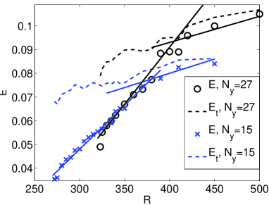
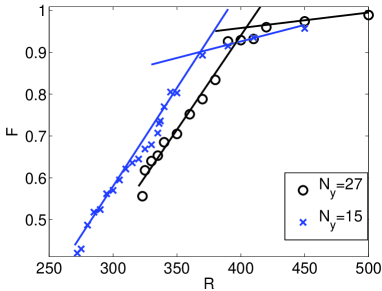
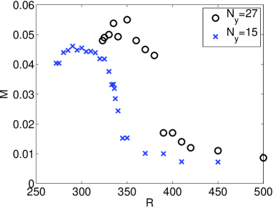
Figure 20: Turbulent quantities $E$, $E_{t}$ (left) and $F$ (center), order parameter $M$ as function of $R$ for a domain of size $L_{x}\times L_{z}=110\times 32$ (right), for two resolutions : $N_{y}=27$, $N_{x,z}/L_{x,z}=6$ (circles) and $N_{y}=15$, $N_{x,z}/L_{x,z}=4$ (crosses)

These result are not qualitatively affected by the increase of resolution from $N_{y}=15$ and $N_{x,z}/L_{x,z}=8/3$ to $N_{y}=27$ and $N_{x,z}/L_{x,z}=4$ as can be seen in Figure 20 which compares the results for both resolutions at size $L_{x}\times L_{z}=110\times 32$. The quantitative change is minor and in the expected fashion[13]. The thresholds $R_{\rm g}$ and $R_{\rm t}$ move to approximately $321$ and $390$. The square of the perturbation undergoes an increase of about $10\%$. Apprt from the threshold shift, the turbulent fraction $F$ is little affected by the resolution change. Both $E$ and $F$ display the expected slope-break. Given the uncertainty on the values of $M$ near $R_{\rm t}$, the value $g_{1}\simeq 30$ at $N_{y}=27$ is acceptable. This reassert the validity of our semi-quantitative approach.

Parameter $g_{2}$ has little influence and reasonable results are obtained from $0.001\lesssim\alpha\lesssim 0.003$. This estimate is consistent with the value obtained from the fit of the phase dynamics fit $\alpha/\tau_{0}\sim 4\times 10^{-4}$, (Fig. 7) if we accept Prigent’s finding $\tau_{0}\sim 30\,h/U$ [3, (a,c)]. The variance of the fluctuations of $m$ in the vicinity of $R_{\rm t}$ is also of interest. Let us define:

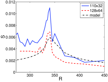
Figure 21: Average root-mean-square fluctuation of $m$ as a function of $R$ for $L_{x}\times L_{z}=110\times 32$ (full line), $128\times 64$ (dashed), and the model with $g_{1}=55$, $g_{2}=250$, $R_{\rm t}=355$, $\alpha=0.002$ (dash-dotted).

$$S^{2}=2\int_{m^{\prime\prime}<m^{\prime}}(m^{\prime}-M)^{2}\Pi(m^{\prime},m^{\prime\prime})\,{\rm d}m^{\prime}{\rm d}m^{\prime\prime}\,.$$

Figure 21 displays the variation of $S$ as a function of $R$. Fluctuations appear to be strongly enhanced in the vicinity of $R_{\rm t}$, due to orientation changes and re-entrance of featureless turbulence. Though model (3) does not account for the latter phenomenon, it already explains a large part of the enhancement. Its parameter $g_{2}$ controls the amplitude of fluctuations that bring about orientation changes. The position of the maximum of $S(R)$ strongly depends on it. With $g_{1}=55$, satisfactory agreement is found for $g_{2}\gtrsim 120$. Results obtained with $g_{2}=250$ are represented as a dash-dotted line in Fig. 21. Including the re-entrance of featureless turbulence would certainly increase the variability but this would still not be the whole story since, like for second order phase transitions, one would expect a divergence of $S$ in the form $S\propto|\tilde{\epsilon}|^{\gamma}$, $\gamma$ being the critical exponent attached to the susceptibility of the order parameter, just rounded off by finite-size effects. Even at reduced numerical resolution, improving the statistics to study the pattern’s fluctuations in the simulations seems presently out of reach.

4 Summary and Conclusion

Prigent et al. [3] have put the problem of the emergence of turbulent bands in wall-bounded flows within the Ginzburg–Landau framework of pattern formation, adding noise to account for background turbulence. Doing so, they were able to extract most of the coefficients in the model equation from laboratory experiments in the case of circular Couette flow, while restricting themselves to threshold localisation and wavelength measurements for PCF. In a similar vein, Barkley et al. [10] later performed simulations of PCF, detecting the formation of bands from Fourier analysis of the pattern. They considered a quasi-one-dimensional configuration excluding orientation fluctuations expected to play a role close to $R_{\rm t}$ for symmetry reasons. Though having the model in mind, they did not attempt any quantitative fit. Our work has been mostly devoted to overcome these two limitations, to check the validity of the noisy Ginzburg–Landau framework, and to compare finding for PCF to those for CCF. Previous result [13] were reasserted, showing that controlled under-resolution gives excellent qualitative agreement with experiments and good quantitative results once corrected for a general shift of the range $[R_{\rm g},R_{\rm t}]$ where the bands are present. We performed numerical experiments in domains of sizes able to contain one to three bands in the spanwise direction and one or two bands in the streamwise direction, while letting the pattern’s orientation fluctuate. Under-resolution reducing the computational load, we could carry out long duration simulations in order to accumulate reliable statistics.

The emergence of bands was first quantitatively characterised using standard statistical quantities such as the total perturbation energy $E$, the turbulent fraction $F$, and the average energy contained in turbulent domains $E_{\rm t}$. These quantities quickly converge to their steady-state values but do not give information on orientation or wavelength fluctuations. This limitation has been next overcome by defining order parameters measuring the amplitude of the modes involved in the Fourier series decomposition of the patterns, appropriately amending the Barkley et al. definitions and procedure. The full nonlinear dispersion relation describing the formation of bands could be studied by varying the Reynolds number and the size of the computational domain which controls the allowed wavevectors. The coefficients of the relevant Ginzburg–Landau equation and the intensity of the noise were estimated, showing the overall consistency of the approach. In particular, two coherence lengths, spanwise and streamwise, were evaluated and the square of the modulation amplitude was shown to vary linearly with $R$ far enough from $R_{\rm t}$, while its fluctuations and the intermittent re-entrance of featureless turbulence were strongly enhanced close to $R_{\rm t}$. It has been argued that the re-entrance of featureless turbulence was a side effect of the limited size of the system, probably explaining the ‘intermittent regime’ of Barkley & Tuckerman [5] by the same token, and that this observation should be better replaced on a spatiotemporal footing in more extended domain, in relation to patterns with mixed orientations observed near $R_{\rm t}$ in CCF experiments [3] or PCF simulations in Fig. 18. Finally, comparing our results with those obtained in CCF we obtain satisfactory general agreement, but with the supplementary information that the streamwise coherence length $\xi_{x}$ is significantly larger than the spanwise coherence length $\xi_{z}$ indicating that the selection of the streamwise wavelength $\lambda_{x}$ is more effective than that of the spanwise wavelength $\lambda_{z}$.

As a whole, the emergence of oblique bands from featureless turbulence upon decreasing $R$ has been seen to fit the conventional framework of a pattern-forming instability. However, the very fact that the base state is turbulent calls for the introduction of a large noise in the picture. These numerical studies are performed with the hope that they will contribute to the understanding of the cohabitation of turbulent and laminar flow typical of the transition to/from turbulence in wall-bounded flows, the detailed mechanism of which is still largely unknown.

References

- [1] (a) D. Cole, Transition in circular Couette flow, J. Fluid Mech. 25, 385–425 (1966). (b) Ch. Van Atta, Exploratory measurements in spiral turbulence, J. Fluid Mech. 25, 495–512 (1966). (c) D. Coles, Ch. Van Atta, Measured distortion of a laminar circular Couette flow by end effects, J. Fluid Mech. 25, 513–521 (1966).
- [2] (a) C.D Anderek, S.S. Liu, H.L. Swinney, Flow regimes in a circular Couette system with independently rotating cylinders, J. Fluid Mech. 164, 155–183 (1986). (b) J.J. Hegseth, C.D. Andereck, F. Hayot, Y. Pomeau, Spiral turbulence and phase dynamics, Phys. Rev. Lett. 62, 257–260 (1989).
- [3] (a) A. Prigent, La spirale turbulente : motif de grande longueur d’onde dans les écoulements cisaillés turbulents, PHD thesis, Université Paris-Sud (2001). (b) A. Prigent, G. Grégoire, H. Chaté, O. Dauchot, W. van Saarlos, Large-scale finite wavelength modulation within turbulent shear slow, Phys. Rev. Lett. 89, 014501 (2002). (c) A. Prigent, G. Grégoire, H. Chaté, O. Dauchot, Long-wavelength modulation of turbulent shear flow, Physica D 174, 100-113 (2003).
- [4] P. Manneville, A. Prigent, O. Dauchot, Banded turbulence in cylindical and plane Couette flow, APS-DFD01 conference, Bull. Am. Phys. Soc. 46 (2001) 35; threshold comparisons reproduced as Fig. 3 in : P. Manneville, Spots and turbulent domains in a model of transitional plane Couette flow, Theor. Comput. Fluid Dynamics, 18 169–181 (2004).
- [5] (a) D. Barkley, L. Tuckerman, Computationnal study of turbulent laminar patterns in Couette Flow, Phys. Rev. Lett. 94, 014502 (2005). (b) D. Barkley, L. Tuckerman, Mean flow of turbulent laminar pattern in Couette flow, J. Fluid Mech. 574, 109-137 (2007).
- [6] Y. Duguet, P. Schlatter, D.S. Henningson Formation of turbulent patterns near the onset of transition in plane Couette flow, J. Fluid. Mech 650, 119–129 (2010).
- [7] A. Meseguer, F. Mellibovsky, M. Avila, F. Marques, Instability mechanisms and transition scenarios of spiral turbulence in Taylor Couette flow, Phys. Rev. E 80, 046315 (2009).
- [8] S. Dong, Evidence for internal structure of spiral turbulence, Phys. Rev. E 80, 067301 (2009).
- [9] T. Tsukahara, Y. Seki, H. Kawamura, D. Tochio, DNS of turbulent channel flow at very low Reynolds numbers, in Turbulence and Shear Flow Phenomena 4 Williamsburg, 2005.
- [10] (a) D. Barkley, O. Dauchot, L. Tuckerman, Statistical analysis of the transition to turbulent-laminar banded patterns in plane Couette flow, J. of Physics, Conference Series 137 012029 (2008) (15th Couette-Taylor Conference, Le Havre, July 2007). (b) L.S. Tuckerman, D. Barley, O. Dauchot, Instability of uniform turbulent plane Couette flow: spectra, probability distribution functions and closure model, in P. Schlatter, D.S. Henningson, eds., Seventh IUTAM Symposium on Laminar-Turbulent Transition (Springer, 2010) pp. 59–66.
- [11] J. Gibson, http://www.cns.gatech.edu/channelflow/.
- [12] J. Rolland, P. Manneville, Oblique turbulent bands in plane Couette Flow: from visual to quantitative data, 16th Couette-Taylor Workshop, Princeton (2009).
- [13] P. Manneville, J. Rolland, On modelling transitional turbulent flows using under-resolved direct numerical simulations, Theor. Comput. Fluid Dyn. in press.
- [14] J. Jiménez, P. Moin, The minimal flow unit in near wall turbulence, J. Fluid Mech. 225, 213–240 (1991).
- [15] S. Bottin, F. Daviaud, P. Manneville, O. Dauchot, Discontinuous transition to spatiotemporal intermittency in plane Couette flow, Europhys. Lett. 43, 171–176 (1998).
- [16] M. Scherer, G Ahler, F. Hörner and I. Rehberg, Deviation from linear theory for fluctuations below the super-critical primary bifurcation to electroconvection, Phys. Rev. Lett. 85, 3754–3760 (2000).
- [17] S. Bottin, H. Chaté, Statistical analysis of the transition to turbulence in plane Couette flow, Eur. Phys. J. B 6, 143–155 (1998).
- [18] B.J. McKeon, K.R. Sreenivasan, eds., Scaling and structure in high Reynolds number wall-bounded flows, theme issue, Phil. Trans. R. Soc. A 365 (2007).
- [19] J. Rolland, P. Manneville, Temporal fluctuations of laminar-turbulent oblique bands in transitional plane Couette flow, J. Stat. Phys, submitted.
- [20] N.G. Van Kampen, Stochastic processes in physics and chemistry (North-Holland, Amsterdam, 1983).