Comment: Quantifying the Fraction of Missing Information for Hypothesis Testing in Statistical and Genetic Studies

10.1214/07-STS244

and

Introduction

The authors suggest an interesting way to measure the fraction of missing information in the context of hypothesis testing. The measure seeks to quantify the impact of missing observations on the test between two hypotheses. The amount of impact can be useful information for applied research. An example is, in genetics, where multiple tests of the same sort are performed on different variables with different missing rates, and follow-up studies may be designed to resolve missing values in selected variables.

In this discussion, we offer our prospective views on the use of relative information in a follow-up study. For studies where the impact of missing observations varies greatly across different variables and where the investigators have the flexibility of designing studies that can have different efforts on variables, an optimal design may be derived using relative information measures to improve the cost-effectiveness of the follow-up.

Using the simple motivation example in their paper, we examine the estimation of relative information by $\mathcal{R}I_{1}$ and $\mathcal{R}I_{0}$ in terms of unbiasedness and variability, and discuss issues that require further research. Although the relative information measure developed in their paper estimates the mean impact of the missing data, the actual impact may be highly variable when the amount of information in the observed data is moderate or small, which makes the estimated mean relative information a less reliable prediction of the actual impact of missing observations. For this reason, we suggest a simple way to estimate the variability of relative information between complete data and observed data in the simple motivation example. Further investigation is required in incorporating these variability estimates into the optimal design of follow-up studies.

Relative Information and Follow-up Study Designs

Missing values can occur for many reasons and can have different effects on a given test. Nicolae, Meng and Kong pointed out that the impact of missing values (in terms of relative information) on a test may not be as simple as the “face value” of $n_{0}/n$, where $n_{0}$ is the number of observed values and $n$ is the number of individuals ($n-n_{0}$ is then the number of missing values). Therefore, a more accurate estimation of the information gain due to the resolution of missing values is important for the design of follow-up studies.

Given an existing data with $n$ individuals (with missing values), if $n_{1}$ additional independent samples are collected (possibly with the same missing rate) to expand this data set, it is intuitive to assume that the ratio of information in the original data and the expanded data is approximately $n/(n+n_{1})$. Now consider a test on the existing data with $n$ individuals that has some missing values (say, $n_{0}$ observed values). The relative information is estimated to be 80%, meaning that if the data used for this test is “resolved” to become complete, the expected log likelihood ratio is about $1/80\%=125\%$ of the observed log likelihood ratio. To achieve the same level of information by adding new independent observations, one would need to collect a sample of additional $n_{1}=n\times 25\%$ individuals. In many situations, resolving missing values, if possible, turns out to be much cheaper than collecting data on additional samples. In Section 2 of the NMK paper, an example was given on genotyping ambiguity in genetic linkage analysis (meaning that the exact inheritance vectors needed for the lod score computation cannot always be derived given the genotypes observed on the individuals). Here, let $Y_{\mathrm{ob}}$ be current data with unambiguous genotypes. For a follow-up study, a researcher can decide between (1) increasing the density of genetic markers on the observed individuals to resolve the ambiguities and (2) increasing the sample size by genotyping more independent individuals on the same set of markers for the previously observed individuals. If we denote the two potential expanded data sets as $Y_{\mathrm{co},m}$ and $Y_{\mathrm{co},i}$ with $m$ and $i$ standing for markers and individuals, we can compute the fraction of information between $Y_{\mathrm{ob}}$ and $Y_{\mathrm{co},m}$, and between $Y_{\mathrm{ob}}$ and $Y_{\mathrm{co},i}$, potentially using $\mathcal{R}I_{1}$ and $\mathcal{R}I_{0}$ proposed in the NMK paper. Comparing these two measures of relative information, the researcher can then decide which option (increasing markers or increasing individuals) is cost-efficient for the inferential task at hand.

In practice, one would need to consider such comparison at multiple variables simultaneously. Here we consider a simple example. Let $\{Y_{1},\ldots,Y_{M}\}$ be the variables studied. For $Y_{i}$, $n_{0,i}$ values are observed on $n$ individuals. In a follow-up study $n_{1,i}$ missing values can be resolved at $Y_{i}$. At $Y_{i}$, the relative information (say, $\mathcal{R}I_{1}$) is a function of $n_{1,i}$, the observed $\mathrm{lod}$ score $\mathrm{lod}_{\mathrm{ob},i}$ and the observed m.l.e. To evaluate the overall information gain due to these additional observations, we suggest an expression similar to that of (19) in the NMK paper:

$$\overline{\mathcal{R}I_{1}}^{-1}(n_{1,1},\ldots,n_{1,M})$$

(1)

$$\quad=\frac{\sum_{i=1}^{M}\mathrm{lod}_{\mathrm{ob},i}\mathcal{R}I_{1}(n_{1,i})^{-1}}{\sum_{i=1}^{M}\mathrm{lod}_{\mathrm{ob},i}}.$$

A possible way to yield an optimal design would be to select values of $0\leq n_{1,i}\leq n-n_{0,i}$ to maximize the information gain while controlling for a fixed cost. Differences in design may involve varying setup costs that may depend on, for example, the number of nonzero $n_{1,i}$ such as that in genotyping studies. Once such a cost function can be fully specified, linear programming can be used to obtain the optimal design. If the $n_{1,i}$’s in the optimal design identified take similar values on $i=1,\ldots,M$, this may suggest a design that collects data on $n_{1}$ new independent individuals and takes measurements on the same $M$ variables as in the original data.

Another advantage of the likelihood ratio-based evaluation of information used by Nicolae, Meng and Kong is that one can evaluate the potential information gain conditioning not only on the observed data at the current concerned variable but also on some associated variables, through a model-based calculation. Similar model-based strategies have been commonly used for imputing missing genotypes in genetic studies. Such consideration may introduce more complicated design questions than the computation in (Relative Information and Follow-up Study Designs) but may also bring better efficiency.

The “Empirical” Fraction of Information and Its Variability

Using the simple motivation example in Section 1 of the NMK paper, we consider the relation between the empirical observed data log likelihood ratio (lod score) and the “random” complete data log likelihood ratio (lod score). We offer relationships between the proposed fraction of information and the distribution of the “empirical” ratio. The “empirical” ratio is the actual random gain due to additional observations, while the estimation of relative information and the possible optimal design derived are intended to approximate this random outcome.

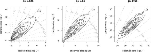
In Figure 1, we plot the joint distribution of the lod scores under the observed data and the complete data, with missing percentage being 80%. The distribution is evaluated under three true values of the probability of success with $n_{0}=800$ and $n=1000$. To obtain a realistic evaluation, we use the traditional definition of the likelihood ratio test (or the lod score) where the ratio is evaluated between the maximum likelihood estimate given current data (observed or complete) and the value in the null hypothesis.

Figure 1: Distribution of log likelihood ratio test statistics (or lod scores) given observed data and complete data. The contour plots display the joint distribution of the log likelihood ratio test statistics given the observed data and the complete data. Given $n_{0}=800$ and $n=1000$, the ratio between the complete data log LR and the observed data log LR is expected to be $n/n_{0}=1.25$. In each contour plot, a dotted line is plotted to indicate the $y=1.25x$ line. The gray broken lines display $y=rx$ with $r$ varying and provide reference for the empirical ratio of the complete data log LR and the observed data log LR.

We first notice the positive correlation between the complete data statistic and the observed data statistic. Gray broken lines in Figure 1 give reference lines for empirical or “random” ratio between the complete data lod score (or log LR statistic) and observed lod score. The estimated $\mathcal{R}I_{1}$ (which coincides with $r=n_{0}/n$) corresponds to a line going through the center of the joint distribution (almost exactly), indicating it is a good estimate for the expected ratio (or fraction of information) regardless of the values of the observed lod score.

For a small departure (say, $p=0.55$) from the null hypothesis ($p_{0}=0.5$), the LR test does not have great power and the test statistics distribute close to zero. The contour of the distribution intersects with lines whose ratio values are shown to go as high as 13. This is natural given the observed data statistic can become very small due to chance and create a highly variable ratio. For values that are far away from the null hypothesis, the estimated $\mathcal{R}I_{1}$ becomes more precise.

Figure 2: Estimated standard deviation of $\mathcal{R}I_{y}^{-1}$. For sample size $n=100,1000$, we plot the estimated standard deviation of $\mathcal{R}I_{y}^{-1}$ against the observed number of successes $x_{0}$. Density curves of observed number of successes $x_{0}$ under different true $p$ values are plotted.

As illustrated above and in Figure 1, the unobserved random missing values make the relative “empirical” information a random quantity. It is instructive to evaluate the amount of variation in the complete data lod score. It is easy to obtain for the simple binomial example that

$$\mathrm{var}[\mathrm{lod}(p_{1},p_{2};Y_{\mathrm{co}})|Y_{\mathrm{ob}},p]$$

(2)

$$\quad=(n-n_{0})p(1-p)\biggl{[}\log\frac{p_{1}}{p_{2}}-\log\frac{1-p_{1}}{1-p_{2}}\biggr{]}^{2}.$$

Consider a null hypothesis that specifies the probability of success as $p_{0}$ and let $p$ be the true parameter value. Let $\mathcal{R}I_{y}(Y_{\mathrm{co}},Y_{\mathrm{ob}};p,p_{0})$ be the empirical fraction of information regarding the difference between $p$ and $p_{0}$, for a set of $Y_{\mathrm{co}}$ with only $Y_{\mathrm{ob}}$ observed (or the ratio of the lod scores between $p$ and $p_{0}$ derived using the observed data and the potential complete data). It is easy to see that $\mathcal{R}I_{y}^{-1}$ is a more natural relative information ratio to use for evaluating overall relative information in (Relative Information and Follow-up Study Designs) and identifying optimal follow-up design. From similar computation in (The “Empirical” Fraction of Information and Its Variability), $\mathcal{R}I_{y}^{-1}$, conditioning on $Y_{\mathrm{ob}}$, has an expectation

$$\mathrm{E}\mathcal{R}I_{y}^{-1}$$

$$\quad=1+(n-n_{0})\biggl{[}p\log\frac{p}{p_{0}}+(1-p)\log\frac{(1-p)}{(1-p_{0})}\biggr{]}$$

$$\qquad\ \,\quad{}\cdot{(\mathrm{lod}(p,p_{0};Y_{\mathrm{ob}}))^{-1}}$$

and variance

$$\mathrm{var}\,\mathcal{R}I_{y}^{-1} = (n-n_{0})p(1-p)\biggl{[}\log\frac{p}{p_{0}}-\log\frac{1-p}{1-p_{0}}\biggr{]}^{2}$$

$${}\cdot{(\mathrm{lod}\left(p,p_{0};Y_{\mathrm{ob}}\right)^{2})^{-1}}.$$

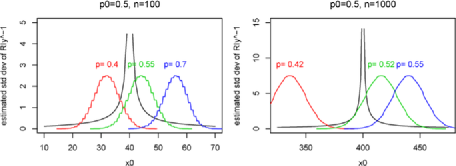
In practice, we may substitute $p$ with $\hat{p}_{\mathrm{ob}}$ and have $\widehat{\mathrm{E}\mathcal{R}I_{y}^{-1}}$ estimated by $\mathcal{R}I_{1}^{-1}$. Figure 2 gives the estimated standard deviation of $\mathcal{R}I_{y}^{-1}$ with probability density curves under different true values of $p$. When the true value is close to the null hypothesis $p_{0}$, $\mathcal{R}I_{y}^{-1}$ is highly variable, which will make the simple estimate of $\mathcal{R}I_{1}^{-1}$ as an estimated expectation of $\mathcal{R}I_{y}^{-1}$ a unreliable prediction of $\mathcal{R}I_{y}^{-1}$. A procedure incorporating both $\widehat{\mathrm{E}\mathcal{R}I_{y}^{-1}}=\mathcal{R}I_{1}^{-1}$ and an estimated standard error of $\mathcal{R}I_{y}^{-1}$ should be considered to address the design issues similar to that of (Relative Information and Follow-up Study Designs).

In Summary

The paper by Nicolae, Meng and Kong provides interesting evaluation strategies for relative information discerning two hypotheses contained in observed data. Such measures support the quantification of possible information gain that can be brought by additional observations, which can be used to optimally design follow-up efforts. The measures $\mathcal{R}I_{1}$ and $\mathcal{R}I_{0}$ deserve more research for further understanding. More importantly, theory and practiceshould be incorporated to provide design suggestions that utilize relative information such as $\mathcal{R}I_{1}$ and corresponding variability measures.