Efficient and scalable geometric hashing method for searching protein 3D structures

Abstract

As the structural databases continue to expand, efficient methods are required to search similar structures of the query structure from the database. There are many previous works about comparing protein 3D structures and scanning the database with a query structure. However, they generally have limitations on practical use because of large computational and storage requirements.

We propose two new types of queries for searching similar sub-structures on the structural database: LSPM (Local Spatial Pattern Matching) and RLSPM (Reverse LSPM). Between two types of queries, we focus on RLSPM problem, because it is more practical and general than LSPM. As a naïve algorithm, we adopt geometric hashing techniques to RLSPM problem and then propose our proposed algorithm which improves the baseline algorithm to deal with large-scale data and provide an efficient matching algorithm. We employ the sub-sampling and Z-ordering to reduce the storage requirement and execution time, respectively. We conduct our experiments to show the correctness and reliability of the proposed method. Our experiment shows that the true positive rate is at least $0.8$ using the reliability measure.

1 Introduction

In this paper, we focus on searching geometrically similar proteins on protein structural database. Geometric similarity on protein 3D structures are known to be highly conserved during evolutions compared to one dimensional amino-acid sequence identity [7]. Therefore, some proteins with different sequences may indeed share the same or highly similar functionality, or proteins with high sequence homology may have different functionality [15]. Our proposed framework, by using the protein 3D structure, detects similar proteins with non-homologous sequences as well.

The structure-based search identifies the pairs with high structural similarities with the following two types: (1) whole structure similarity comparing global structures and (2) sub-structure similarity comparing similar sub-structures shared by the pairs. In this paper, we focus on the sub-structure similarity, as it is studied to be more appropriate than whole structure similarity, for finding functionally related proteins [12]. This finding can be explained by the fact that proteins with similar global structures may not share similar functionality when their functional regions, or sub-structures, such as active or binding sites are different [13].

More specifically, this paper studies the problem of searching similar proteins to the given query protein, which can be retrieved by the following two types of queries. First, one can use a sub-structure of protein, or a patch, as a query and retrieve the proteins with the similar 3D structures. We name this type of query LSPM (Local Spatial Pattern Matching), where a query pattern is much smaller than proteins in the database. Second, one can use a protein as a query and search the sub-structure databases, which we call RLSPM (Reverse LSPM).

We aim at developing an efficient method for RLSPM. Between the two problems, LSPM and RLSPM, we focus on the latter, as it is more (1) practical yet (2) general. First, regarding practicality, while LSPM requires the prior knowledge on a query protein, by requiring users to identify “meaningful” query patches from a protein as a query. To ensure high-quality results, those patches should be related to protein functions, which is hard to know in advance for a protein with an unknown function. Second, regarding generality, RLSPM can be considered to be more general, in the sense that its solution can straightforwardly be used to answer LSPM, as the two problems are essentially the same, except whether query patterns are relatively larger (RLSPM) or data pattern instances are (LSPM). However, while databases readily offer efficient access methods for large data instances, e.g., indices, it is more challenging to efficiently support large query structures. In that sense, a solution to LSPM, not considering large queries, is likely to incur huge costs when applied to RLSPM. However, an efficient solution to RLSPM designing a sophisticate approach to consider large query patterns will efficiently answer LSPM as well.

This paper proposes a framework for RLSPM based on geometric hashing technique. Our proposed framework, by identifying matches sharing functionally important regions, can contribute to predicting the functions of newly discovered proteins and moreover to designing more effective drugs. More specifically, we summarize the contributions of our paper as follows:

• We develop an efficient and effective way to adopt geometric hashing for our target problem of RLSPM.

• We study an incremental maintenance scheme for grid structure to accommodate the insertion of large protein structures.

• We extensively validate our proposed framework over large-scale data using both annotated and non-annotated proteins as queries.

The rest of the paper is organized as follows. We presents the representation of protein 3D structure and naïve adoption of geometric hashing technique to our problem in Section 2. Next, we describe our proposed method in Section 3. Section 4 presents our experimental results. Section 5 concludes our work and presents some future work.

2 Preliminary

2.1 Representation of protein 3D structure

A widely adopted representation of the protein 3D structure used in prior works is based on an approximation using $C_{\alpha}$ and a pseudo atom (the centroid of the side chain). This representation approximates all the atoms in the side chain to one pseudo atom to reduce both time and space complexity for protein comparison methods. However, this approximation is not appropriate of our target problem focusing on functional region, as atoms in side chains, among all the atoms, are generally associated with the functional regions [2]. Therefore, approximating atoms in the side chain compromises the precision of the results.

In a clear contrast, we represent the 3D structures using all the atomic coordinates for query proteins and patches, in order not to compromise the precision. As adopting this representation increases the time and space complexity, we will develop algorithms and access methods to optimize such cost as we will describe in Section 3.

2.2 Naïve algorithm based on geometric hashing technique

This section develops a naive algorithm as a baseline approach, adopting geometric hashing to identify functional regions of a query protein by scanning the patches in the database.

The geometric hashing technique [5] was invented originally for object recognition in the field of computer vision, which has been adopted to compare protein 3D structures as well in many previous studies [6, 4, 14, 9]. In [6] and [4], they adopted geometric hashing to identify substructures (3D motifs) of a query protein, which are nearly identical with substructures of proteins in the database. Pennec and Ayache proposed a comparison method for two given proteins. It can be extended to the comparison of a query protein with proteins in the database [9]. TESS [14] used geometric hashing for the problem similar to LSPM, searching proteins in the database which contain user defined substructure.

In contrast, our target problem is RLSPM, assuming a large-scale database of 3D substructures (patches), on which a whole 3D protein structure is used as a query. While straightforwardly adopting the geometric hashing technique can be a solution to our problem, this naïve approach incurs both space and time complexity. In Section 3, we will discuss the drawbacks of this naïve approach in details, then we will propose algorithms significantly outperforming it.

More specifically, the geometric hashing can be adopted to our target problem in the following two steps–the preprocessing step and the matching step. First, the preprocessing step is applied to all patches to generate a GH table dividing a whole space into equal-sized cells occupied with atoms. The origin is located at the center of GH table and each cell contains the information of atoms belonging to the cell, which will be used in the next step. Then, the preprocessing step proceeds to generate all possible coordinates system (CS). The CS is determined by three non-collinear atoms, which can be one of $n(n-1)(n-2)$ possible combinations for a patch with $n$ atoms. To distinguish CSs, we assign each CS a unique number (hereafter we call it rfid) then we store all possible combinations (rfid and coordinate) of atoms into the corresponding cells.

Second, the matching step is to find similar patches for a given query protein. The GH table built on the patch database is matched with a set of transformed atoms by each CS of a query protein. As a result, we obtain a list of rfid pairs (rfid of the patch database, rfid of a query protein) which have matching scores larger than a user-defined threshold value. In the matching step, a matching is carried out by searching the cell of GH table corresponding to an atom of the query protein. If an atom $q_{i}$ of the query protein is located in a non-empty cell $C_{j}$ of the GH table, we consider that $q_{i}$ is matched with all atoms in $C_{j}$. The matching score of rfid pair is the number of matched atoms divided by the number of atoms in the patch. The matching step is repeated for all possible CSs of the query protein.

3 Method

This section describes how to efficiently evaluate the RLSPM query. We provides enhancement strategies for two steps of geometric hashing technique. Based on these enhancement strategies, we design our proposed algorithm.

3.1 Preprocessing step

This section discusses the first step of our proposed algorithm, in which all the atoms of each patch are transformed and inserted into a GH table for all possible coordinate system.

Contrast to the naïve algorithm, we adopt the sub-sampling scheme to reduce the space requirement of GH table. More specifically, we define one CS for each residue using just three atoms ($C_{\alpha}$, N, and C atoms) of a residue. A unique number is assigned for each CS. We call it rfid as in geometric hashing method. For each atom transformed by a CS, we insert coordinates of the atom and rfid of the CS into the cell of GH table corresponding to the coordinates of the atom.

Recall that the naïve algorithm requires the space complexity $O(n^{4})$ for each protein 3D structure where $n$ is the number of atoms. However, in the proposed preprocessing step, the total number of CS is equal to to the number of residues in protein 3D structure. With the sub-sampling, the space complexity is reduced to $O(nm)$ where $n$ is the number of atoms and $m$ ($<n$) is the number of residues.

In addition to sub-sampling, we also build a disk-based GH table to ensure the scalability to handle a large-scale data beyond the size of memory. In a disk-based GH table, cells are stored in a secondary memory instead of a main memory. As a result, the size of GH table is not restricted within that of main memory.

After we insert all patches in the database into GH table, we then sort the cells of GH table in the order of z-value [8], which enables single access per each cell during matching step. A z-value is assigned to each cell according to its location, and all cells in GH table are sorted in the order of z-value. The z-value is easily calculated by interleaving bit-strings of each axis– When comparing two cells in two GH tables, we can use this unique value to easily determine whether the two cells are in the same location.

3.2 Matching step

We now move on to discuss our second step of retrieving similar patches in the database for the given query protein. In particular, we first build a GH table for the given query protein, then match the rfid of query protein with the rfids of the patches in the database. We then retrieve all the matches with matching score higher than the given threshold.

As a matching score, we use the ratio of the number of overlapped cells in a query protein with the cells in a patch to the number of cells in a patch. Note our matching score is defined in the level of cells and not in the level of atoms. However, we can adjust the cell size $\delta$, to decrease to obtain the results with high accuracy or to increase for efficiency.

With the matching score metrics, we now describe the overall structure of our algorithms. First, a GH table is built for a query protein with the similar way of the preprocessing step. The only difference from building the GH table for patch database is that we only consider atoms within $P_{max}$ from origin. We set $P_{max}$ to the size of the largest patch, the size of matches is always less than $P_{max}$. Hereafter we call the GH table of a query protein $G_{q}$ and the GH tableof patch database $G_{p}$. Second, for each GH table, the cell with the smallest z-value is loaded into the main memory. As the GH table was sorted in the order of z-value, this is done by scanning each GH table in the sorted order. During this scan, z-values of current two cells are checked– If the z-value of a cell from $G_{p}$ is bigger than that from $G_{q}$, the next cell of $G_{q}$ is fetched into the memory and the equality test is performed again for a newly loaded cell.

When the two cells have the same z-values, we update the matching scores between all rfid pairs of a patch and a query protein. Update can be done by adding the number of atoms with the same rfid in a cell of $G_{p}$ to the previous score of each rfid of a query protein. The matching scores are stored in a temporary file (hereafter called the score table) in case its size is too large to keep in the main memory.

After the above update processes for all the overlapped cells, all the values in the score table, i.e., rfid of patch database, rfid of a query protein, is divided by the size of the patch corresponding to rfid of patch database. The size of patch is the number of all atoms in it. From the score table, we extract only the rfid pairs with matching scores higher than the given threshold value called protein-patch threshold $S_{patch}$. In other words, our proposed algorithm will report the sub-regions of a query protein which are structurally similar to some patches with higher matching scores than $S_{patch}$.

4 Experimental results

In this section, we first describe how to build the patch database from existing databases such as PDB [3] and CSA [10] in Section 4.1. We then validate the reliability of our proposed algorithm over all protein 3D structures from PDB. More specifically, for the proteins without annotated patches, we compute reliability using ‘keyword recovery’ used in the field of protein-protein interaction (Section 4.2).

4.1 Protein Patch Database

In this section, we discuss how we build PPD (Protein Patch Database), by extracting functional regions (patches) from two existing protein structure databases, i.e., PDB and CSA.

First, PDB [3] contains the 3D coordinates of atoms and functional information. For some proteins in this database with “known” functional regions, residues directly involved with those regions are annotated (in ‘SITE’ record). We collected atomic coordinates for those residues, i.e., $9206$ patches, inserted into PPD.

Second, CSA [10] contains enzyme active sites and catalytic residues in enzymes, based on the functional annotations of PDB and SWISS-PROT database. More specifically, CSA provides two types of structural templates– Ca/Cb atom template and functional atom template. A Ca/Cb atom template provide only Ca or Cb atom coordinates and a functional atom template provide atomic coordinates of directly related atoms to interact its substrates. In particular, we use the Ca/Cb atom template of CSA version $1.0$ to obtain functionally important residues. For these residues, we then generate a patch, by extracting atomic coordinates belong to those residues, i.e., $147$ templates in CSA version $1.0$. Among them $34$ templates were identical to the patches extracted from PDB as CSA is based on PDB. We remove such duplicates and insert the remaining $113$ patches of CSA into PPD.

4.2 Reliability analysis against non-annotated protein

In this section, we discuss our validation using non-annotated proteins. Non-annotated proteins mean that there is no patch annotated on them. Therefore, when using the non-annotated proteins as queries, the matching results are expected to contain matching pairs of a query protein and matching patches that are not annotated on the query protein.

We first discuss the measure that can be used to analyze the reliability of the results when using non-annotated proteins as queries. We will then show our reliability results.

As a reliability metric, we adopt ‘keyword recovery’ [11] used in the field of PPI (Protein-Protein Interaction) for validating results. More specifically, this metric compares the annotation keywords of two proteins and calculates the true positive (TP) rate. As performing in vivo or in vitro experiments to validate the functional relationships of every pair is infeasible, we adopt this indirect measure instead.

The TP rate is calculated by following formula [11].

$$TP=(D-R)/(I-R)$$

where $D$ is the ratio of pairs with the same keywords from the given dataset. $R$ is the ratio of pairs with the same keywords among all pairs in the given dataset. $I$ is the ratio of pairs with the same keywords in true matching pairs. We set $I$ to $1$ as in [11].

To adopt the ‘keyword recovery’ method, annotated keywords are needed for query proteins and patches. We use keywords about the biological process and cellular component in Gene Ontology [1]. In case of the patch, we use keywords of the protein from which the patch has been extracted, because there is no annotation for a particular patch.

Using the reliability measure, we calculate the true positive rate for the matching result which is a list of matching pairs with higher matching scores than $S_{patch}$. In addition to $S_{patch}$, we introduce an another parameter $S_{pro}$ that restricts matching pairs whose structural identity is bigger then $S_{pro}$ to eliminate the redundancy in the matching result. We perform our algorithm to compute structural identity between the query protein and the protein from which “matched” patch is extracted. If the score between two proteins is bigger than some threshold value ($S_{pro}$), two proteins are regarded as same protein and corresponding matching pair is thrown away from the result set for validation.

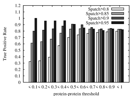
Figure 1: True Positive rate by various threshold values

Figure 1 shows the TP rates for varying $S_{patch}$ and $S_{pro}$. We only present the results when the biological process is used as keywords. Because there are few entries on which cellular components are annotated, we omit the result of cellular component. We consider $S_{patch}$ to be in the range from $0.8$ to $0.95$. When $S_{patch}$ is low, it frequently occurs for a query protein to be matched with a patch by chance. This means lots of meaningless matching pairs could be included in the result. Therefore, We remove those matching pairs from the result by setting $S_{patch}$ to a value higher than $0.8$.

As $S_{patch}$ and $S_{pro}$ is set to $0.8\sim 0.95$ and $0.1\sim 1$ respectively, we calculate the TP rates of the results given by two threshold values. As shown in Figure 1 The TP rates decrease for lower value of $S_{patch}$ when $S_{pro}$ is less than $0.5$. This observation indicates that the number of pairs (query protein, patch) which are matched by chance increases according as $S_{patch}$ is decreasing. As $S_{patch}$ increases (i.e. more precise matching) overall TP rate also increases. This shows the specificity of functional site.

Two parameters, $S_{patch}$ and $S_{pro}$ have influence on the reliability of the matching result. We recommend that $S_{patch}$ is set to the value between $0.9$ and $1$. Because the interaction between proteins generally has high specificity, the structural similarity between a query protein and a patch should be high to obtain the meaningful matching results. For $S_{pro}$, we recommend users to set it according to the application. Our experiment shows that the TP rate is at least $0.8$ when $S_{pro}$ and $S_{patch}$ are set as our recommendation.

5 Conclusion

In this paper, we study sub-structure similarity search on protein 3D structural database. We present two types of sub-structure similarity search: LSPM and reverse LSPM. Between them, we focus on reverse LSPM problem because it is more practical and general then LSPM. Toward the goal, we introduced our improved algorithm which significantly outperforms adopting geometric hashing technique “as is” in terms of both storage overhead and execution time. More specifically, to reduce storage overhead, we applied a sub-sampling technique to coordinate system set and developed a disk-based GH table for accommodating a large scale of query protein patches in the database. Furthermore, to reduce execution time, we restricted a query structure within a reasonable range, namely within maximum patch size, and employed the Z-ordering to eliminate redundant accesses which requires only a single access per a cell of GH table by concurrently scanning two GH table sorted in the order of z-values.

The reliability of proposed method was validated using our protein patch database which we build by extracting annotated residues from PDB and CSA. The true positive rate is at least $0.8$ under recommended parameter value. We are in the process of validating the reliability of our method over other protein structural database such as protein-protein interface database [16].

References

- [1] Michael Ashburner, Catherine A. Ball, Judith A. Blake, David Botstein, Heather Butler, J. Michael Cherry, Allan P. Davis, Kara Dolinski, Selina S. Dwight, Janan T. Eppig, Midori A. Harris, David P. Hill, Laurie Issel-Tarver, Andrew Kasarskis, Suzanna Lewis, John C. Matese, Joel E. Richardson, Martin Ringwald, Gerald M. Rubin, and Gavin Sherlock. Gene ontology: tool for the unification of biology. Nat Genet, 25(1):25–29, 2000.
- [2] Gail J. Bartlett, Craig T. Porter, Neera Borkakoti, and Janet M. Thornton. Analysis of catalytic residues in enzyme active sites. Journal of Molecular Biology, 324(1):105–121, 2002.
- [3] Helen M. Berman, John Westbrook, Zukang Feng, Gary Gilliland, T. N. Bhat, Helge Weissig, Ilya N. Shindyalov, and Philip E. Bourne. The Protein Data Bank. Nucl. Acids Res., 28(1):235–242, 2000.
- [4] D. Fischer, H. Wolfson, S. L. Lin, and R. Nussinov. Three-dimensional, sequence order-independent structural comparison of a serine protease against the crystallographic database reveals active site similarities: Potential implications to evolution and to protein folding. Protein Sci, 3(5):769–778, 1994.
- [5] Yehezkel Lamdan and Haim J. Wolfson. Geometric hashing: A general and efficient model-based recognition scheme. In Proc. Computer vision, pages 238–249, Dec 1988.
- [6] R. Nussinov and H. J. Wolfson. Efficient Detection of Three-Dimensional Structural Motifs in Biological Macromolecules by Computer Vision Techniques. Proceedings of the National Academy of Science, 88:10495–10499, December 1991.
- [7] Christine A Orengo, Annabel E Todd, and Janet M Thornton. From protein structure to function. Current Opinion in Structural biology, 9(3):374–382, 1999.
- [8] Jack A. Orenstein and T. H. Merrett. A class of data structures for associative searching. In PODS, pages 181–190, 1984.
- [9] X Pennec and N Ayache. A geometric algorithm to find small but highly similar 3D substructures in proteins. Bioinformatics, 14(6):516–522, 1998.
- [10] Craig T. Porter, Gail J. Bartlett, and Janet M. Thornton. The catalytic site atlas: a resource of catalytic sites and residues identified in enzymes using structural data. Nucl. Acids. Res, 32:D129–D133, 2004.
- [11] E. Sprinzak, S. Sattath, and H. Margalit. How reliable are experimental protein-protein interaction data? J Mol Biol, 327(5):919–923, April 2003.
- [12] William R. Taylor and David T. Jones. Templates, consensus patterns and motifs. Current Opinion in Structural Biology, 1(3):327–333, 1991.
- [13] A. Via, B. Brannetti F. Ferrè, and M. Helmer-Citterich. Protein surface similarities: a survey of methods to discribe and compare protein surfaces. Cellular and Molecular Life Sciences, 57(13/14):1970–1997, 2000.
- [14] Andrew C. Wallace, Neera Borkakoti, and Janet M. Thornton. Tess: A geometric hashing algorithm for deriving 3d coordinate templates for searching structural databases. application to enzyme active sites. Protein Science, 6(11):2308–2323, 1997.
- [15] James C. Whisstock and Arthur M. Lesk. Prediction of protein function from protein sequence and structure. Quarterly Reviews of Biophysics, 36(3):307–340, 2003.
- [16] Christof Winter, Andreas Henschel, Wan Kyu Kim, and Michael Schroeder. Scoppi: a structural classification of protein-protein interfaces. Nucleic Acids Research, 34(Database-Issue):310–314, 2006.