X-ray emission and dynamics from large diameter superbubbles: The case of N 70 superbubble

Abstract

The morphology, dynamics and thermal X-ray emission of the superbubble N70 is studied by means of 3D hydrodynamical simulations, carried out with the yguazú-a code. We have considered different scenarios: the superbubble being the product of a single supernova remnant, of the stellar winds from an OB association, or the result of the joint action of stellar winds and a supernova event. Our results show that, in spite that all scenarios produce bubbles with the observed physical size, only those where the bubble is driven by stellar winds and a SN event are successful to explain the general morphology, dynamics and the X-ray luminosity of N70. Our models predict temperatures in excess of $10^{8}~{}\mathrm{K}$ at the interior of the superbubble, however the density is too low and the emission in thermal X-ray above $2~{}\mathrm{keV}$ is too faint to be detected.

1. Introduction

Massive OB stars, or groups of them (young clusters or OB associations) inject a large amount of mechanical energy via stellar winds and violent supernova (SN) episodes to the interstellar medium (ISM). They sweep-up their environment producing the so-called bubbles and superbubbles (when they are produced by a single star, or multiple stars, respectively). The standard models of these bubbles are those by Weaver et al. (1977), and Chu & Mac Low (1990). They consider the mechanical energy input of a stellar wind, and predict an extended bubble structure of shock-heated gas that emits mainly in X-rays, surrounded by a cool shell of swept-up material that is bright at optical wavelengths. These models has been compared with several observations, and the X-ray observed luminosities often exceed the theoretical predictions (i.e. Chu & Mac Low 1990, Wang & Helfand 1991).

Later, Oey (1996b) based on the observations of Rosado et al. (1981, 1982), and Rosado (1986) proposed two categories of superbubbles: high-velocity and low-velocity ones. The high-velocity superbubbles are characterized by a shell expansion velocity $v_{s}\gtrsim 25~{}\mathrm{km~{}s^{-1}}$, and they are as common as the low-velocity ones (e.g. Rosado 1986). The difference, however, lies in the fact that it is virtually impossible to obtain expansion shell velocities in excess of $25~{}\mathrm{km~{}s^{-1}}$ in superbubbles with large diameters (about 100 pc) without additional acceleration (e.g. an impact from a supernova remnant, SNR). The energy injected by SN explosions would be an extra source of heating for the gas inside the superbubble and this could explain the observed X-ray excess.

In this work we have turned our attention to the superbubble N 70 in the Large Magellanic Cloud (LMC). N 70 is an almost circular superbubble of approximately 50 pc in radius. The superbubble is driven by the OB association LH 114 (Lucke & Hodge 1970), which contains more than a thousand stars. Oey (1996a) classified seven of them as a O-type stars and estimated the mean age of the OB association to be around 5 Myr. Rosado et al.(1981) and Georgelin et al. (1983) found [SII]/H$\alpha$ line-ratios in N 70 with values larger than those in photoionized H II regions, but lower than those of SNR in the LMC. The measured expansion velocity of this superbubble ($\sim 70~{}\mathrm{km~{}s^{-1}}$) is consistent with shock models that also reproduce the [S II]/H$\alpha$ ratio of Rosado et al. (1981). However, the dynamical age derived with this velocity does not agree with the model of Oey (1996b).

Reyes-Iturbide et al. (2011) calculated the thermal X-ray luminosity for the superbubble N 70 (DEM 301), with the XMM-Newton observations from Jansen et al. (2001). For the analysis of the X-ray spectrum they used the three individual data sets adjusting them jointly. They extracted spectra from each of the three EPIC/MOS1, EPIC/MOS2 and EPIC/PN event files. The spectra were fitted with a two-component model consisting of a thermal plasma-MEKAL (Kaastra & Mewe 1993), and nonthermal power law. The resulting spectra were analyzed jointly using the XSPEC spectral fitting package, where the fit has an absorption column density of $N_{H}=1.4\pm 0.5\times 10^{20}$ cm^-2 (in agreement with the measures of column densities in the LMC direction, see Dickey & Lockman 1990). The X-ray luminosity in the 0.2-2 keV energy band with absorption-corrected was found to be 1.6$\times$10³⁵ erg s^-1.

Here, we present a series of 3D numerical simulations of the N 70 superbubble using the physical properties (stellar types, positions, etc.) of the stellar cluster in its interior. We analyze the resulting morphology, dynamics and thermal X-ray emission, and compare it with observations of N 70. The paper is organized as follows. In Section 2 we provide a brief review of the models and theoretical predictions of the emission in superbubbles. In Section 3 we describe the numerical simulations, the results of the simulations are analyzed in Section 4, and a summary is provided in Section 5.

2. Superbubble dynamics and X-ray emission

Table 1Coordinates and spectral types of the most massive stars inside N 70

Star	RA	DEC	spectral type	$V_{\infty}$	$\log\left(\dot{M}\right)$
	[hr min sec]	$[\arcdeg~{}\arcmin~{}\arcsec]$		$[\mathrm{km~{}s{{}^{-}1}}]$	$[\mathrm{M}_{\odot}~{}\mathrm{yr}^{-1}]$
D301-1005	5 43 08.33	-67 50 52.5	O9.5 V	1500	-6.9
D301SW-1a	5 43 15.50	-67 51 09.7	O8 III(f)	2000	-6.6
D301SW-1b	5 43 15 50	-67 51 09.7	O9: V	1500	-6.8
D301SW-3	5 43 12.87	-67 51 16.3	O3 If	4100	-4.90
D301NW-4	5 43 17.70	-67 50 36.6	O5: III:e	2900	-6.2
D301NW-8	5 43 15.98	-67 49 51.2	O7 V((f))	2000	-6.6
D301NW-9	5 43 24.60	-67 50 31.1	O9.5 V	1500	-6.9
D301NE-5	5 43 34.85	-67 50 40.9	B0.5 V	2000	-7.25
D301NW-12	5 43 23 79	-67 50 21.5	BO V	2000	-7.3
D301NW-13	5 43 06.71	-67 49 56.0	B1 V	1700	-6.51
D301SW-9	5 43 10.03	-67 52 21.3	B1.5: V	900	-5.26
D301NW-15	5 43 12.25	-67 50 52.8	B1.5V	900	-5.26
D301NW-18	5 43 11.13	-67 50 40.3	B0 V	2000	-7.3

Let us consider a simple model of superbubble formation, where the stars deposit the total mechanical energy in form of stellar winds. Such mechanical luminosity is given by

$$L_{w}=\sum^{N}_{i=1}\frac{1}{2}\dot{M}_{w,i}v^{2}_{w,i}\,,$$ (1)

where, $\dot{M}_{w,i}$ and $v_{w,i}$ are the mass-loss rate and the wind terminal velocity of the $i$-th star, and $N$ is the total number of stars. At the beginning, the stellar winds inside the cluster volume collide with the surrounding ISM (here we will assume a uniform medium with preshock number density “$n_{0}$”) forming shells of shocked ISM material. At some point the volume between the stars fills with shocked material from the individual stars and the winds coalesce into a common cluster wind that forms a larger shell, a “supershell” (Cantó et al. 2000, Rodriguez-Gonzalez et al. 2008, etc.). As the supershell expands with respect to the cluster center, one can distinguish a superbubble structure with four regions:

1. A free wind region, formed by unperturbed stellar wind, which is only found around the most powerful stars.

2. A shocked wind region, formed by the interaction of several individual stellar winds. This material has been heated enough that it emits primarily in X-rays.

3. An outer region of swept-up interstellar medium with an important optical line emision.

4. The unperturbed ISM medium (of uniform density of $n_{0}$), just outside the swept-up shell.

The X-ray luminosity that arise from the internal shocked region, where the gas temperature is in the range of 10⁶-10⁷ K ($\sim 0.1-2$ keV), can be estimated as in Weaver et al. (1977) and Chu & Mac Low (1990) :

$$L_{X}=3.29\times 10^{34}I(\tau)\xi L^{33/35}_{37}n^{17/35}_{0}t^{19/35}_{6}\,\,\,[{\rm erg\,s^{-1}}]$$ (2)

where

$$I(\tau)=\frac{125}{33}-5\tau^{1/2}+\frac{5}{3}\tau^{3}-\frac{5}{11}\tau^{11/3},~{}\mathrm{and}$$ (3)

$$\tau=0.16L^{-8/35}_{37}n^{-2/35}_{0}t^{6/35}_{6}.$$ (4)

$\xi$ is the gas metallicity, $L_{37}=L_{w}/10^{37}$, $t_{6}=t/10^{6}$, $L_{w}$ is the mechanical luminosity of the cluster, and $t$ is the cluster lifetime. If a supernova explodes at the center of stellar cluster, the total X-ray luminosity will be modifed as estimated by Chu & Mac Low (1990) :

$$L(SNc)_{X}=8\times 10^{33}\xi h(x_{s})(1-x_{s})^{-2/5}L^{33/35}_{37}\\$$

$$\;\;\;\,\,\,\,\,n^{17/35}_{0}t^{19/35}_{6}\,\,\,[{\rm erg\,s^{-1}}]$$ (5)

where, $x_{s}=r_{s}/R$, $r_{s}$ is the radius of the remnant, $R$ is the radius of the superbubble, and

$$h(x)=\frac{125}{156}-\frac{5}{13}(1-x)^{13/5}+\frac{5}{4}(1-x)^{8/5}\\$$

$$-\frac{5}{3}(1-x)^{3/5}.$$ (6)

However, as mentioned above, observed X-ray luminosities exceed these predictions. In order to explain such differences several alternatives have been explored, for instance: Chu & Mac Low (1990) have proposed an off-centered supernova explosion, Silich et al. (2001) studied effects of metallicity enhancement (due to evaporation of the outer shell) and Reyes-Iturbide et al. (2009) considered the interaction of the cluster wind with a high density region in the ISM for the case of M 17.

For N 70, the total mechanical luminosity injected by the stellar winds of massive stars (the most massive are listed in Table 1) is around 7.31$\times$10³⁷ erg s^-1. This superbubble evolves in an ISM with number density $\sim$0.16 cm^-3 (Rosado et al. 1981 and Skelton et al. 1999), and an average gas metallicity is $\sim 0.3\mathrm{Z}_{\odot}$ (typical of the LMC, Rolleston, Trundle & Dufton 2002). N 70 is quite circular with a radius of $\sim$50 pc, using the shell expansion velocity a dynamical age of $\sim$3$\times$10⁵ yr can be obtained. Using these values in the equations 2 and 5, the predicted X-ray luminosity for this object is 3.32$\times$10³⁴ erg s^-1 when only the stellar winds are taken into account, and 3.68$\times$10³⁴ erg s^-1 if one adds a single centered SN to the cluster wind.

The X-ray luminosities predicted by the standard models are an order of magnitude less than the observed value. The difference seems to large to be explained by the metallicity effects as proposed by Silich et al. (2001), and the ISM around it is fairly homogeneous (unlike in M 17 where the inhomogeneity of the medium suffices to explain the X-ray luminosity). In addition, Oey (1996b) showed that is essentially impossible to obtain expansion velocities ($\gtrsim$25 km s^-1) in superbubbles with radius of a few tens of parsecs without induced acceleration (a SNR impact was proposed in that paper). Thus, given the high X-ray luminosity and expansion velocity we chose to consider an off-centered SN explosion, with the restriction that it can not be too far from the center because the quasi-spherical shape of N 70. The SN possibility is also consistent with the stellar population models N 70 presented by Oey (1996b) where 13 massive stars are found the range form 12 to 40 M_⊙). A $\sim$60 M_⊙ star could be expected using a standard initial mass function of N 70, and if formed with the rest of the cluster, it would already have exploded as a SN.

Table 1 shows the coordinates and spectral types of the most massive stars inside N 70. In the same table, we have included characteristic values of the terminal wind speed and mass loss rate associated with stars of such spectral types (de Jager et al. 1988, Wilson & Dopita 1985, Leitherer 1988, Prinja et al. 1990, Lamers & Leitherer 1993, Fullerton et al. 2006).

3. The numerical models

Figure 1.— The stellar distribution of $xy$-plane (top panel) and x-z plane (bottom panel) for all the numerical models.

In order to estimate the X-ray emission and shell dynamics in N 70, we have computed 3D numerical simulations with the full, radiative gas dynamic equations. We use a tabulated cooling function obtained with the CHIANTI  database, using a metallicity $\xi$=0.3 Z_⊙ (consistent with that the LMC, see Rolleston, Trundle & Dufton 2002). The simulations include multiple stellar wind sources in the 3D adaptive grid yguazú-a code, which is described in detail by Raga et al. (2000, 2002). They were computed with a maximum resolution of 0.4296 pc (corresponding to $256^{3}$ grid points at the maximum grid resolution) in a computational domain of 110 pc (along each of the 3 coordinate axis). We have not included thermal conduction effects in any of our models.

In all runs, we assumed that the computational domain was initially filled by a homogeneous ambient medium with temperature $T_{0}=$ 10⁴ K (as it would be expected in the photoionized region around the massive OB association) and density $n_{0}=0.16$ cm^-3. The stellar winds are imposed in spheres of radius $R_{w}=7.94\times 10^{18}$ cm ($\sim$0.58 pc), corresponding to 6 pixels of the grid. Table 1 gives the position of the stars in equatorial coordinates (J2000), which can be translated to parsecs considering that the cluster is at a distance of 50 kpc. Then the wind sources are placed in the $xy$-plane according to their positions in the sky. Since we do not know the individual line-of-sight distance ($z$-coordinate) to the stars, we produced randomly picked positions in $z$, retaining the same $xy$ configuration. The $z-$distribution was obtained from a pseudo random sampling to yield a $\propto R^{-2}$ distribution (similarly to Reyes-Iturbide at al 2009). The maximum of the distribution from which the z positions were sampled was set to the maximum separation in the plane of the sky. Figure 1 shows the stellar distribution in the $xy$-plane (top panel) and $xz$-plane (bottom panel) for all the numerical models. Inside the spheres centered at the star positions a stationary wind is imposed (at all times) with an $\propto R^{-2}$ density profile scaled to yield the $V_{\infty}$ and $\dot{M}$ for each star, and a constant temperature $\propto V^{2}_{\infty}$.

We ran four numerical models, M1, M2, M3 and M4 to explore the efects of the mechanical energy injected by the stellar winds and the supernova explosion in the superbubbles dynamics and X-ray emission. The properties of the models are presented in Table 2. In model M1, we considered the energy injected by a single SN (with 10⁵¹ erg) in an homogeneous ISM. In model M2 included the mechanical energy injected by the stellar winds alone. Models M3 and M4 explore the combined effect of stellar winds and a SN explosion. For model M3 we included the energy injected by a SN (similar to that in M1) inside the wind blown bubble (as model M2) at the center of the stellar population of N 70. The SN detonation was imposed at t=1.15$\times$10⁵ yr. Finally, in model M4 we explored the effects of a SN slightly off-center, the SN explosion was placed at (1.5, -1.5, -1.5) pc from the center of the stellar distribution, also at t=1.15$\times$10⁵ yr.

Table 2Numerical models general properties

Model	Winds	SN	SN Location
M1	no	yes	Center
M2	13 stars	no	no
M3	13 stars	yes	Center
M4	13 stars	yes	Off-center

4. Results

4.1. Superbubble dynamics

In order to obtain the physical flow configuration we computed the radially dependent flow density, radial velocity and temperature averaging over spherical concentric surfaces $S_{R}=4\pi R^{2}$ (see also Rodríguez-González et al. 2007):

$$\rho_{a}(R)={1\over 4\pi}{\int_{S_{R}}\rho\,\sin\theta\,d\theta d\phi}\,,$$ (7)

Figure 2.— The spherically averaged flow from model M1. the density (top), temperature (center) and radial velocity (bottom) obtained from the numerical simulation is shown as a function of spherical radius $R$. The dashed lines represent the position of the maximum value of the shell density.

$$v(R)={1\over 4\pi\rho_{a}(R)}{\int_{S_{R}}\rho v_{R}\,\sin\theta\,d\theta d\phi}\,,$$ (8)

$$T(R)={1\over 4\pi\rho_{a}(R)}{\int_{S_{R}}\rho T\,\sin\theta\,d\theta d\phi}\,,$$ (9)

where $\theta$ and $\phi$ are the polar and azimuthal angles, respectively, $\rho$ is the flow density, $T$ the temperature and $v_{R}$ the radial velocity (obtained by projecting the three cartesian velocity components resulting from the numerical integration onto the direction normal to the spherical surface). That is $v_{R}=(xv_{x}+yv_{y}+zv_{z})/R$.

Figures 2, 3 and 5 show the superbubble and shell distributions of density, temperature and radial velocity (top, middle and bottom panel) for model M1, M2 and M3, respectively, at an evolutionary time of 2$\times$10⁵ yr. Model M1 (see Figure 2) forms a thin shell with maximum density at R=47 pc. This shell contains the interstellar medium that has been swept up by the leading shock produced by the explosion. The gas behind the leading shock cools and forms the thin shell. There the temperature is around 10⁵ K, in the range of optical line emission. At the radius at which the density is maximum the radial velocity is around 75 km s^-1. This model does not include the stellar wind contribution and the radial velocity drops because of the interior of the bubble is cooling radiatively (the supernova remnant has past the Sedov phase and it is well into the radiative one).

Figure 3.— Same as Figure 2 but for the model M2.

The contribution of the stellar winds of the cluster in the shell dynamics is present in Figure 3. Model M2 (see Figure 3 and 4) presents a thick shell with a maximum density at R=44 pc. This shell is driven by the mechanical energy injected by stellar winds inside the cluster volume in the form of a common cluster wind (Cantó et al. 2000, Rodríguez-González et al. 2008, etc.).

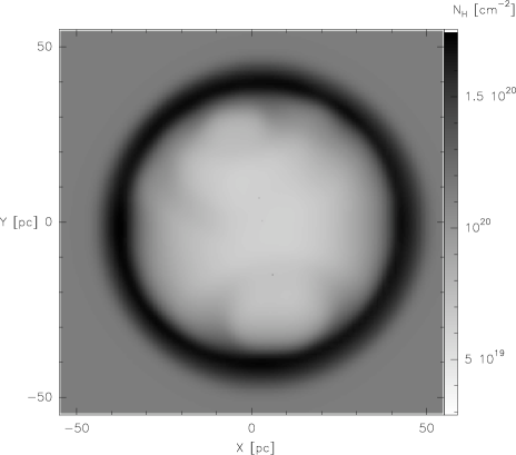
Figure 4.— The column density for model M2 at t=2$\times$10⁵ yr.

Figure 3 shows a average temperature (inside the shell) of 5$\times$10⁵ K (optical line emission regime) and the radial velocity at the density peak is around 45 km s^-1 as predicted by the standard model of Weaver et al. 1977 (see also Chu et al. 1995). This velocity is, however, lower than that obtained from the observations of N 70 by Rosado et al. (1981).

Models M3 and M4 correspond to model M2 until t=1.15$\times$10⁵ yr, at which point we inject a SN (centered for M3, off-center for M4). Figure 5 shows the distributions of density, temperature and radial velocity as function of radius for model M3. From the density profile we obtain a shell position between 43 and 52 pc from the center, with a peak density around R=47 pc. The temperature is adequate for X-ray emission inside a region of 41 pc in radius. The radial velocity profile show an average value in the shell around $\sim$62 km s^-1. This velocity is close to the observed value.

Figure 5.— Same as Figure 2 but for model M3.

Since in M4 the SN not centered one can not assume radial symmetry and radial averages (eqs. 7-9 ) are not longer appropriate. However, in order to estimate an average radial velocity of the shell in this model, we used the equation 8 and the average radial velocity in shell is $\sim$66 km s^-1 (see the velocity profile of this model in Figure 6), similar to that of M3 model, and also similar to N 70 observations.

Figure 6.— The spherically averaged radial velocity flow from model M4, obtained from the numerical simulation as a function of spherical radius $R$. The dashed lines represent the position of the maximum value of the shell density.

5. H$\alpha$ and X-ray emission

From the results of the simulations we computed H$\alpha$ maps, integrating the emission coefficient along the $x$-axis. The emission coefficient is obtained with the interpolation formula given by Aller (1987) for the temperature dependence of the recombination cascade.

We also made X-ray emission maps, using the density and temperature distributions from the simulations and plugging them into the CHIANTI atomic data base and software (see Dere et al. 1997, Landi et al. 2006).The maps are obtained integrating the X-ray emission coefficient along the $z$-axis. For this calculation, it is assumed that the ionization state of the gas corresponds to coronal ionization equilibrium in the low density regime (i. e. the emission coefficient is proportional to the square of the density). The emission has been separated into three energy bands [$0.2-2$], [$2-10$], and [$10-20$] keV. The emission coefficient for this energy bands as a function of temperature is presented in Figure 7.

Figure 7.— X-ray emission coefficients in the [$0.2-2$], [$2-10$], [$10-20$] keV energy ranges (solid, dotted and dashed lines respectively) as function of the temperature.

We also calculated the X-ray emision for all the models as function of time. All our models cover a evolutionary time of 2$\times$10⁵ yr, corresponding approximately to the dynamical age of the superbubble derived by Rosado et al. (1981). In Figure 8 we present the X-ray luminosity, in the energy range of 0.2 to 2 keV for M1, M2, M3 and M4. For visual purposes the horizontal axis of M1 (where the SN was initiated at $t=0$) was shifted to coincide with the SN starting point of models M3 and M4 (t=1.15$\times$10⁵ yr). From the figure one can see that the X-ray luminosity for model M2 has a maximum value of L${}_{X}\sim$4$\times$10³⁴ erg s^-1 (5 times less energy as observed) reached at t=5$\times$10⁴ yr. After this time the luminosity slowly declines.

Figure 8.— X-ray luminosity (between 0.2 to 2 keV) as function of time, for models M1, M2, M3 and M4 (solid, dotted, dashed and dot-dashed lines respectively. The calculated X-ray luminosities of model M1 was shifted by $\Delta t=$1.15$\times$10⁵ yr, in order to compare the its X-ray luminosity values with the X-ray luminosities of M3 and M4 after the supernova explosion

The rest of the models, in which we have included a SN, reach X-ray luminosities of $>10^{35}$ erg s^-1 (see Table 3). In model M1, the highest value of the X-ray luminosity is $\sim$3$\times$10³⁵ erg s^-1, and this luminosity is kept at or above the N 70 observed value for $\sim$5$\times$10⁴ yr. However, when this model reaches the observed radius value of N 70 ($\sim$50 pc, at t=2$\times$10⁵ yr), the X-ray luminosity has dropped by more than 2 orders of magnitude below the observed value.

Table 3Models results

	$v_{s}$	LX,rs	tLx	$\Delta$tLx	LX,max
	[km s-1]	[1035 erg s-1]	[105 yr]	[103 yr]	[1035 erg s-1]
Obs.	70	1.6	2.4	–	–
M1	90	$\sim$ 2.0	2.7	52	3.76
M2	$\sim 45$	$\sim$ 0.21	–	–	0.364
M3	$\sim 67$	$\sim$ 0.48	1.20	2.0	1.02
M4	$\sim 75$	$\sim$ 1.00	1.18	75	1.96

The maximum X-ray emission in model M3 can reach $10^{35}$ erg s^-1, but it is still significantly lower than the observed luminosity, and when the superbubble reaches the observed radius the X-ray luminosity is already 5 times smaller. A centered supernova explosion at t=10⁵ yr (when the shell is closer to the center of the stellar cluster) could help to reach the N 70 X-ray emission, but by the time it reaches a 50 pc radius the luminosity would be down to a value of $\sim 3\times$10³⁴ erg s^-1 (comparable to model M2).

The maximum X-ray luminosity, in model M4, is $\sim$2$\times$10³⁵ erg s^-1, and this luminosity is above the observed value for a timescale of $\sim$7.5$\times$10⁴ yr. By the time the superbubble reaches a radius of $\sim$50 pc the X-ray luminosity agrees well with the observations.

In Figure 9 we show synthetic X-ray emission maps for model M2. The emission in the figure has been separated into three energy bands $0.2-2$, $2-10$, and $10-20$ keV (from top to bottom, panels (a), (b), and (c), respectively). It is readily evident that the emission is dominated by soft X-rays with only a small contribution from harder X-rays. For this model (M2) the emission in the soft X-ray band ($0.2-2$ keV) is three orders of magnitude larger than the emission in the $2-10$ keV energy range and over five orders of magnitude larger than the harder X-ray emission ($10-20$ keV). The fact that the emission in hard X-rays negligible with respect to that in soft X-rays might seem surprising at a first glance, considering that there is a large region (inner $30$ pc) filled with 10⁸ K gas, which should emit in hard X-rays (see the emission coefficients in Figure 7). However, the density at the interior of the bubble is quite low, and it is only beyond $\sim 30$ pc that it increases (rapidly) with radius, at the same temperature drops to ${\sim 10^{7}~{}\mathrm{K}}$. Since the thermal X-ray emission is proportional to the density squared the result is that most of the emission observed arises from close to the shell, form a region cold enough to produce soft X-rays.

Temperatures of 10⁸ K have been observed and modeled in super stellar clusters (Silich et al. 2004 and 2005), which are much more massive that the young star association in N 70. The reason for such temperatures is the high terminal velocity of some of the winds ($>2000~{}\mathrm{km~{}s^{-1}}$). The difference is that in super stellar clusters the density of stars is significantly larger, thus the gas density inside is enough to produce an observable amount of hard X-rays. In contrast, the massive stars in N 70 are too far apart each other and the emission above $2~{}\mathrm{keV}$ is very faint compared with that at lower energies.

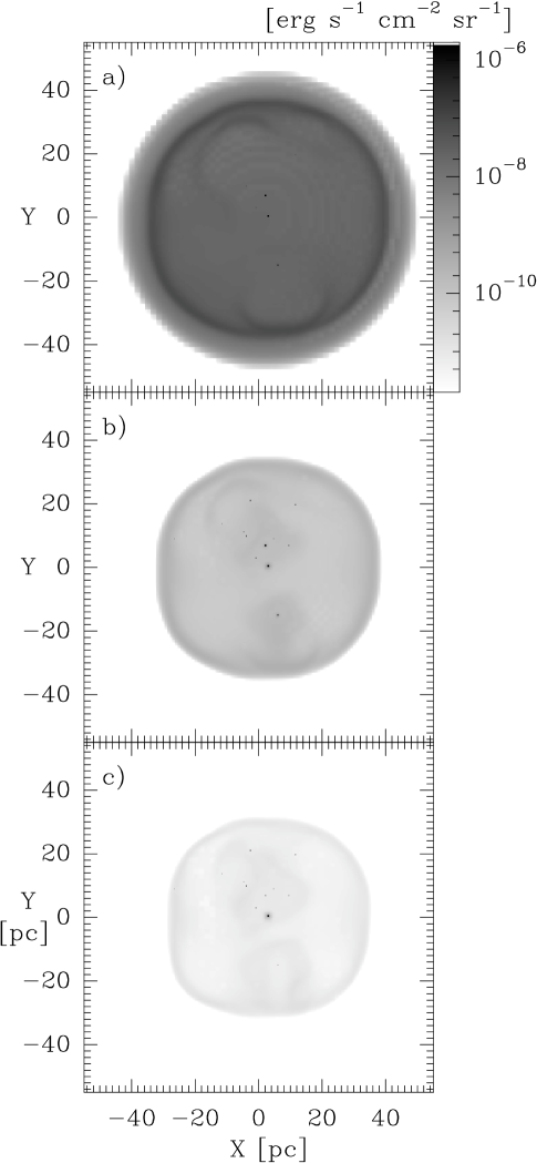
Figure 9.— Synthetic X-ray emission map of model M2 in the (a) [$0.2-2$] keV, (b) [$2-10$] keV, and (c) [$10-20$] keV energy ranges.

Figure 10 shows the H$\alpha$ map and superposed X-ray isocontours of M4 model. The X-rays isocontours cover a wide range of flux of energy from 10^-9 to 10^-6 erg cm^-2 s^-1 sr^-1 in steps of 5$\times$10^-8 erg cm^-2 s^-1 sr^-1. The highest values of the isocontours are at the center and in a shell just behind (inside) the optical superbubble (between 38 to 47 pc). The outer shell or superbubble is formed by the interaction of the cluster wind and its surrounding ISM.

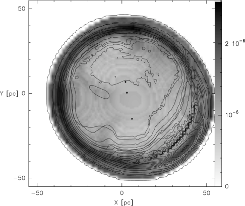
Figure 10.— Overlay of the simulated H$\alpha$ emission map (grays) with contours of the synthetic X-ray emission.

Table 3 present a summary of the numerical results for the dynamics and X-ray luminosities obtained from our models. In this table we include the evolutionary time when the maximum X-ray luminosity is reached for each model ($t_{Lx}$) and the interval that the X-ray luminosity is kept above 10³⁵ erg s^-1 ($\Delta$t_Lx).

In our models we did not include the thermal conduction effects. Weaver et al. (1977) and several other authors (Chu & Mac Low 1995, Silich et al. 2001 etc.) have recently studied its importance to explain the total X-ray emission in stellar clusters and SNRs. However, Silich et al. (2001) shows that while thermal conduction might have produce an enhancement of several orders of magnitude in superbubbles with ages $>$10 Myr, for young superbubbles (such as N 70) thermal conduction can only produce a difference of a factor of $\sim 5$. It is important to notice that the main effect of thermal conduction is to carry material from the external shell into the bubble, thus filling the bubble with X-rays, and maintaining its emission for a longer time (see also Silich et al. 2001). This is because thermal conduction drives a transfer of the material from the external shell to the center of the bubble.

The standard model of bubbles (Weaver et al. 1977) predicts X-ray emission from the hot interior of bubbles by including thermal conduction effects. Its success is controversial because in some cases the predicted X-ray luminosities where lower than detected (as in the case of the N70 superbubble) while, in other cases, the predicted X-ray emission is higher than detected (as in the case of the M17 superbubble; Dunne et al. 2003, Reyes-Iturbide et al. 2009). The new results on thermal conduction effects mentioned above make us believe that thermal conduction is not the main ingredient originating the difference. In this work we propose that the inclusion of a supernova explosion, as an additional agent to be considered besides the stellar winds, is more important than thermal conduction. At least two reasons could be given in order to support this: (1) In the case of M17, it is almost certain that no SN explosion has occurred yet while the age of LH114, at the interior of N70, makes plausible a SN explosion, and (2) the expansion velocities predicted by Weaver et al. (1977) model in the case of N70 are much lower than the measured velocities for this superbubble. As seen in Figures 2 to 5 and Table 3 only the models including a SN explosion predict a shell acceleration that could explain large expansion velocities as the ones measured in high-velocity shells, such as N70. Thus, we suggest that the main difference between high velocity and low velocity superbubbles is the occurrence (or lack) of a SN explosion in their interiors. Off-centered explosions can change some of the detailed structure and dynamics, but the main conclusions remain unchanged. Of course, we have explored only the N70 superbubble and we need to study in detail other superbubbles (both of high and low-velocity types)in order to confirm this suggestion.

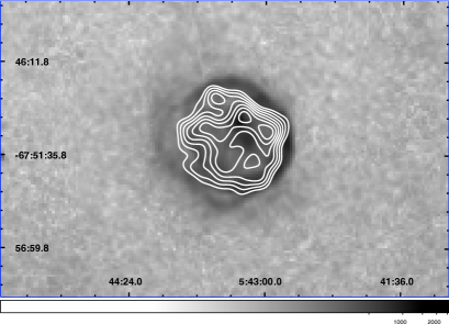
Figure 11.— The Halpha MCELS image of N70 (grays) is overlaid with X-ray contours. Contours have been drawn at levels of 3 , 4 , 5 , 6 , 7 , 8 , 9 and 10 above the background level.

6. Conclusion

We have studied the dynamics and X-ray emission of superbubbles driven by cluster winds including in our models supernova explosions alone, stellar winds alone, and a combination of stellar winds and SN explosions, these latter at different times and locations. We have turned our attention to the superbubble N 70 in order to confront our model predictions with the observations. We computed four models (M1-M4) of superbubbles using the properties of the more massive stars contained in the cluster inside the N70 superbubble, adopting the ISM density and metallicity around this superbubble. The models are evolved in a homogeneous (in density and temperature) medium.

From our models we demonstrated that the case in which only the stellar winds inject mechanical energy (M2), the soft X-ray luminosity is lower by an order of magnitude than the observed value (in agreement with the standard model). And the radial velocity of the shell is less than 45 km s^-1. However, the model of a single supernova explosion (M1), even when the input from stellar winds is not considered, could reach the X-ray luminosity and an expansion velocity consistent with the observations. Nevertheless, a single SN explosion predicts the formation of a very thin shell which is not in agreement with the morphology of the N 70 superbubble.

Three models considered the mechanical energy injected by stellar winds, M2 only considers the input from stellar winds, while M3 and M4 have been combined with a SN explosion. We included the SN explosion at two different positions, near to the cluster center, and $\sim$2 pc from the cluster center (M3 and M4 respectively). The SN has exploded after t=1.15$\times$10⁵ yr of the evolutionary time of the cluster wind. From models M3 and M4 we can obtain an X-ray emission in good agreement with the observational data during 20 and 75 kyr, respectively. And the shell velocity expansion ($\sim$60 km s^-1), obtained in both models, could explain the kinematics measured for this bubble. Models M3 and M4 formed a thick shell, also in agreement with the observations of N 70.

As a matter of fact, both models M3 and M4 reproduce quite well the large measured expansion velocity of the N70 shell and the X-ray luminosity. Model M4 lacks spherical symmetry because the off-centered SN, however, the morphological difference is somewhat subtle and it can be concealed for certain orientations with respect to the line of sight. So, we cannot discard it. Figure 10 shows the predicted H$\alpha$ emission (gray levels) and the X-ray emission (isocontours) for the M4 model and Figure 11 depicts the observed ones showing good agreement.

It is important to notice that our models predict a large region inside the superbubble (the innermost $\sim 30~{}\mathrm{pc}$) with temperatures $\gtrsim 10^{8}~{}\mathrm{K}$, which would result in thermal hard X-ray emission (above $2~{}\mathrm{keV}$). However the density inside the superbubble is very low and it produces only a faint emission that is overwhelmed by the soft X-rays produced in the surrounding shell.

We end by noting that in this paper we did not include the thermal conduction effects. However, for young superbubbles, with ages less than 10 Myr (as well as N 70) the differences between models with and without thermal conduction are only on a factor of $\sim 5$ in $L_{X}$ (Silich et al. 2001). A more important role of thermal conduction in superbubble models is the fact that it helps sustain the X-ray emission for longer periods of time.

References

- (1) Aller, L. H., 1987, Physics of Therma Gaseous Nebulae (Dordrecht: Reidel), pp. 76-77.
- (2) Cantó, J., Raga, A.C. & Rodríguez, L.F., 2000, ApJ, 536, 896.
- (3) Chu, Y.-H., Chang, H.-W., Su, Y.-L. & Mac Low, M.-M., 1995, ApJ, 450, 157.
- (4) Chu Y.-H. & Mac Low M.-M., 1990, ApJ, 365, 510.
- (5) de Jager, C., Nieuwenhuijzen, H. & van der Hucht, K. A., 1988, A&AS, 72, 259.
- (6) Dere, K. P., Landi, E., Mason, H. E., Monsignori Fossi, B. C. & Young, P. R., 1997, A&AS,125, 149.
- (7) Dickey, J. M. & Lockman, F. J., 1990, ARA&A, 28, 215.
- (8) Dunne, B. C., Chu, Y.-H., Chen, C.-H. R., Lowry, J. D., Townsley, L., Gruendl, R. A., Guerrero, M. A. & Rosado, M., 2003, ApJ, 590, 306.
- (9) Fullerton, A. W., Massa, D. L. & Prinja, R. K., 2006, ApJ, 637, 1025
- (10) Georgelin, Y. M., Georgelin, Y. P., Laval, A., Monnet, G. & Rosado, M.,1983, A&AS, 54, 459.
- (11) Jansen, F., Lumb, D., Altieri, B., Clavel, J., Ehle, M., Erd, C., Gabriel, C., Guainazzi, M., Gondoin, P., Much, R., Munoz, R., Santos, M., Schartel, N., Texier, D. & Vacanti, G. 2001, A&A, 365, L1
- (12) Kaastra, J. S. & Mewe, R., 1993, Legacy, 3, 16.
- (13) Lamers, H. J. G. L. M. & Leitherer, C., 1993, ApJ, 412, 771.
- (14) Landi, E., Del Zanna, G., Young, P. R., Dere, K. P., Mason, H. E. & Landini, M., 2006,ApJS, 162, 261.
- (15) Leitherer, C., 1988, ApJ, 326, 356.
- (16) Lucke, P. B.& Hodge, P. W., 1970, AJ, 75, 171.
- (17) Prinja, R. K., Barlow, M. J. & Howarth, I. D., 1990, ApJ, 361, 607.
- (18) Oey, M. S., 1996a, ApJ, 465, 231.
- (19) Oey, M. S., 1996b, ApJ, 467, 666.
- (20) Raga, A. C., Navarro-González, R. & Villagrán-Muniz, M., 2000, Revista Mexicana de Astronomía y Astrofisíca, 36, 67.
- (21) Raga, A. C., de Gouveia Dal Pino, E. M., Noriega-Crespo,A., Mininni, P. D. & Velázquez, P. F. 2002, A& A, 392, 267.
- (22) Reyes-Iturbide, J., Rosado, M. & Velázquez, P. F., 2008,AJ, 136, 2011.
- (23) Reyes-Iturbide, J., Velázquez, P. F., Rosado, M., Rodríguez-González, A., González, R. F., & Esquivel, A. 2009, MNRAS, 394, 1009
- (24) Reyes-Iturbide, J., Rosado, M., Velázquez, P. F., Rodríguez-González, A. & Esquivel, A., 2011, AJ, submitted (Paper I).
- (25) Rodríguez-González, A., Cantó, J., Esquivel, A., Raga, A. C. & Velazquez, P. F., 2007, MNRAS, 380, 1198.
- (26) Rodríguez-González, A., Esquivel, A., Raga, A. C. & Cantó, J., 2008, ApJ, 684, 1384.
- (27) Rolleston, W. R. J., Trundle, C. & Dufton, P. L. 2002, A&A, 396, 53.
- (28) Rosado, M., 1986, A&A, 160, 211.
- (29) Rosado, M., Georgelin, Y. P., Georgelin, Y. M., Laval, A. & Monnet, G., 1981, A&A, 97,342.
- (30) Rosado, M., Georgelin, Y. M., Georgelin, Y. P., Laval, A. & Monnet, G., 1982, A&A, 115, 61.
- (31) Silich, S., Tenorio-Tagle, G., Terlevich, R., Terlevich, E. & Netzer, H., 2001, MNRAS, 324, 191.
- (32) Silich, S., Tenorio-Tagle, G.,& Rodríguez -González A., 2004, ApJ, 610,226.
- (33) Silich, S., Tenorio-Tagle, G.,& Añorve-Zeferino, A., 2005, ApJ, 635, 1116.
- (34) Skelton, B. P, Waller, W. H., Gelderman, R. F., Brown, L. W., Woodgate, B. E., Caulet, A. & Schommer, R. A., 1999, PASP, 111, 465.
- (35) Wang, Q. D. & Helfand, D., 1991, ApJ, 379, 327.
- (36) Weaver, R., McCray, R., Castor, J., Shapiro, P. & Moore, R., 1977, ApJ, 218, 377.
- (37) Wilson, I. R. G. & Dopita, M. A. 1985, A&A, 149, 295.