X-ray mass proxies from hydrodynamic simulations of galaxy clusters (paper I)
Abstract
Using extended sets of cosmological hydrodynamical simulations of galaxy clusters, we present a detailed study of scaling relations between total cluster mass and three mass proxies based on X–ray observable quantities: temperature of the intra–cluster medium, gas mass and the product of the two, . Our analysis is based on two sets of high–resolution hydrodynamical simulations performed with the TreePM–SPH GADGET code. The first set includes about 140 cluster with masses above , with 30 of such clusters having mass above . All such clusters have been simulated in two flavours, with both non–radiative physics and including cooling, star formation, chemical enrichment and the effect of supernova feedback triggering galactic ejecta. The large statistics offered by this set of simulated clusters is used to quantify the robustness of the scaling relations between mass proxies and total mass, to determine their redshift evolution, and to calibrate their intrinsic scatter and its distribution. Furthermore, we use a smaller set of clusters, including 18 halos with masses above , four of which are more massive than , to test the robustness of mass proxies against changing the physical processes that are included in the simulations to describe the evolution of the intra–cluster medium. Each cluster is simulated in seven different flavours to study the effect of (i) thermal conduction, (ii) artificial viscosity, (iii) cooling and star formation, (iv) galactic winds, and (v) AGN feedback.
As a general result, we find the – scaling relation to be the least sensitive one to variations of the ICM physics, its slope and redshift evolution being always very close to the predictions of the self–similar model. As for the scatter around the best–fitting relations, its distribution is always close to a log-normal one. is the mass proxy having the smallest scatter in mass, with values of –0.06, depending on the physics included in the simulation, and with a mild dependence on redshift. As for the mass–temperature relation, it is the one with the largest scatter, with at , increasing to at . The intrinsic scatter in the – relation is slightly larger than in the – relation, with at and 0.08 at . These results confirm that both and mass proxies are well suited for cosmological applications of future large X–ray surveys. As a word of caution, we point out that the analysis presented in this paper does not include observational effects expected when measuring temperature from fitting X–ray spectra and gas mass from X–ray surface brightness profiles. A detailed assessment of such effects will be the subject of a forthcoming paper.
keywords:
Cosmology: Miscellaneous – Methods: Numerical – X–rays: Galaxies: Clusters.1 INTRODUCTION
Measuring the mass of galaxy clusters represents the most important aspect for the use of such structures as tracers of cosmic evolution. The cosmological parameters depend, indeed, on the evolution of cluster’s mass function and on large–scale clustering properties (e.g., Borgani et al., 2001; Schuecker et al., 2002; Voit, 2005a; Vikhlinin et al., 2009; Mantz et al., 2010). Restricting the discussion to X–ray observations, to estimate cluster masses we need to assume that the intra–cluster medium (ICM) sits in hydrostatic equilibrium within the cluster potential well, generally assumed to have spherical simmetry. Further, we need to obtain gas density and temperature profiles from high–quality X–ray data. Limits on this approach are represented not only by the strong assumptions made but also by the difficulty of obtaining data of sufficient quality. This is especially true for distant clusters, at , for which observations of the needed sensitivity would be prohibitively expensive in terms of required exposure time.
To overcome this problem one generally resorts to the observational determinations of mass proxies, i.e. of suitably observable quantities easier to measure and related to total cluster mass through the so-called “scaling relations”. Ideally, a robust mass proxy should be characterized by a low intrinsic scatter with cluster mass, implying that it neeeds to be relatively insensitive to the cluster dynamical state. Different examples of X–ray mass proxies have been used over the last decade to derive cosmological constraints from X–ray clusters surveys. The easiest-to-measure mass proxy is the total X–ray luminosity, . While this quantity is known to correlate with cluster mass (e.g., Reiprich & Böhringer, 2002; Pratt et al., 2009), the – relation has a fairly large scatter, of about 40 per cent, due to the sensitivity of X–ray luminosity on the details of the gas distribution in central regions and, therefore, on the dynamical state of the cluster. Other commonly adopted choices of mass proxies are the X–ray temperature (e.g. Henry & Arnaud, 1991; Markevitch, 1998; Ikebe et al., 2002; Pierpaoli et al., 2003) and the cluster gas mass (e.g. Vikhlinin et al., 2003; Voevodkin & Vikhlinin, 2004). In order to estimate these quantities detailed X–ray brightess profiles must be obtained, requiring longer exposure times than those required by only. However, they are expected to be more robustly linked to total collapsed mass.
In this context cosmological hydrodynamical simulations are playing an increasingly relevant role in calibrating the mass proxies, in understanding the systematics on cluster mass measurements, and in defining new mass proxies. Simulations provide the most advanced theoretical tool to capture the complexity of the hierarchical build–up of galaxy clusters and of the gas–dynamical processes (e.g. Borgani & Kravtsov, 2009, for a recent review on cluster simulations). A typical example is provided by the role that simulations played in the last years to calibrate the expected level of violation of hydrostatic equilibrium induced by the presence of non–thermalised gas motions (e.g., Rasia et al., 2004; Nagai et al., 2007; Jeltema et al., 2008; Ameglio et al., 2009; Piffaretti et al., 2010; Lau et al., 2009). Another example is given by the application of simulations in the study of the accuracy of X–ray temperature and of gas mass as tracers of the total cluster mass (e.g., Evrard et al., 1996; Bartelmann & Steinmetz, 1996; Muanwong et al., 2006; Ettori et al., 2004; Nagai et al., 2007). With the increasing numerical resolution and degree of realism of the physical processes included, these calibrations are becoming trustworthy as convincingly shown by different works. A good match between simulations and observations was shown for temperature profiles of clusters (e.g., Loken et al., 2002; Borgani et al., 2004; Kay et al., 2007; Nagai et al., 2007; Leccardi & Molendi, 2008), gas density profiles (e.g., Roncarelli et al., 2006; Croston et al., 2008) and pressure density (e.g., Arnaud et al., 2009).
These comparison are mostly restricted to the region within 111We define as the mass contained within the radius encompassing an overdensity of times the cosmic critical density, ., after excluding the central regions affected by the complex physical processes regulating the “cool core” structure of the ICM.
As for the cluster mass proxies simulations predict that the – relation has an intrinsic scatter which is quite sensitive to the presence of substructures in the ICM and to the cluster dynamical state (e.g., O’Hara et al., 2006; Yang et al., 2009). The gas mass proxy is instead expected to be less sensitive to the cluster dynamical state, thus implying a smaller scatter in its scaling relation with total mass. Moreover it has the advantage that it can be essentially measured from X–ray imaging alone. There is however a caveat, since the dependence of gas mass fraction on cluster mass, cluster-centric distance and on redshift are still not yet completely understood (e.g., Ettori et al., 2006).
Kravtsov et al. (2006) introduced the X–ray equivalent of the integrated SZ flux, the parameter, defined as the product of the gas mass with the cluster temperature. From a set of sixteen simulated galaxy clusters these authors found it to be a low–scatter (5-8 per cent) mass proxy, due to the anticorrelation of the residuals in the scaling relation of temperature and gas mass with total mass. Furthermore, the scaling of with total mass was found to be in close agreement with the prediction of the simple self–similar model, based on the assumption that gas follows dark matter and gravitational effects only determine the thermal content of the ICM (e.g., Kaiser, 1986). The – relation is relatively insensitive to cluster mergers, a result that was independently verified by Poole et al. (2007) and by Rasia et al. (2010) with simulations of cluster mergers. A number of recent observational works estimated and its correlation with X–ray luminosity. Data from both XMM-Newton Pratt et al. (2009) and Chandra telescope Vikhlinin et al. (2009); Maughan (2007) showed that the observed – relation has slope and redshift evolution in agreement with predictions of the self–similar model. With their sample of both nearby and distant clusters out to , they confirm that gravitational processes are indeed responsible for the bulk of the total thermal content of galaxy clusters.
A more recent analysis of scaling relations for simulated galaxy clusters presented by Stanek et al. (2010) did not confirm the anti–correlation of the residuals of and . They found that the lowest-scatter mass proxy is . A similar result was also found by Okabe et al. (2010) who computed the scaling relation between X–ray mass proxies and the total cluster mass obtained from lensing observations of 12 clusters at . From their analysis the conclusion is that has the lowest intrinsic scatter of , with respect to the of the proxy.
At present, , and are considered the most robust indicators of cluster mass and, in fact, the most recent cosmological applications of X–ray cluster surveys have been based on the use of such mass proxies (e.g., Henry et al., 2009; Vikhlinin et al., 2009; Mantz et al., 2010).
Ideally, rather than relying on simulations, it would be preferrable to calibrate mass proxies directly from observational data. An observational calibration, while possible in principle, requires highly precise measurements of cluster mass in a way which is completely independent of X-ray observations, e.g. from gravitational lensing or from the study of the cluster internal dynamics as traced by member galaxies. Indeed, any determination of the scatter between any of the above three X-ray mass proxies and cluster mass based on the application of hydrostatic equilibrium would be just inconclusive, owing to the fact that the relation is between two highly correlated quantities. On the other hand, precise measurements of lensing masses are now available only for a relatively small number of objects (e.g., Mahdavi et al., 2008; Zhang et al., 2010; Okabe et al., 2010). Although progresses in this direction are expected in the future, simulations represent today a valid alternative to calibrate mass proxies and to understand their robustness.
A careful study of mass proxies through simulations requires a large enough sample of clusters simulated both with adequate resolution and by including a range of physical processes. The most direct way to achieve large statistics of clusters would be to carry out simulations of large cosmological boxes (e.g. Borgani et al., 2004; Gottloeber et al., 2006; Kay et al., 2007; Burns et al., 2008; Hartley et al., 2008). However, these simulations have to severely compromise between box size, achievable resolution and details with which different physical processes (e.g., star formation and feedback from different sources) can be studied. As an alternative, one could simulate at high resolution only specific regions surrounding clusters, which are previously identified from low-resolution simulations of large cosmological volumes. The advantage of this approch is that it can provide a more realistic numerical description, in terms of resolution reached and of physical processes included, only within the “zoomed-in” Lagrangian regions surrounding clusters. As a matter of fact, this resimulation procedure is non-trivial to implement, thus limiting the statistics of resimulated clusters so-far presented in the literature. For instance, Dolag et al. (2009) presented a set of such clusters, of which however only have (see also Fabjan et al., 2010). Lau et al. (2009) and Puchwein et al. (2008) presented sets of resimulated clusters of comparable size, again with only a couple of them being as massive as .
In this paper we use two sets of simulated clusters, whose combination provides us with both a large statistics of massive objects and a range of physical processes included over which to test the stability of the scaling relations. The first set of clusters (Set 1 hereafter) contains about 140 clusters, 30 of which have masses larger than . For all of them, we carried out simulations with both non–radiative physics and by including cooling, star formation and galactic winds powered by Type-II supernova (Sn-II) explosions. The second set of simulations (Set 2 hereafter) includes 18 clusters, with 4 of them having masses larger than . We refer to Dolag et al. (2009) for a complete description of the second set of simulations. This smaller set of simulated clusters complements the first set since it has been simulated by changing in seven different ways the description of physical processes (e.g. artificial viscosity, cooling, star formation, feedback efficiency from SN and from gas accretion onto supermassive black holes). The complementary analysis of these two cluster sets allows us to address in detail the stability and robustness in the calibration of X–ray mass proxies with simulations, by combining statistics of massive halos, numerical resolution and range of physical processes included.
In this first paper we will carry out an analysis of scaling relation of mass proxies against mass by neglecting all observational effects. For this reason ICM temperature will be mass–weighted (where not listed differently), and all quantities will be estimated in a three–dimensional analysis without including projection effects. In this way, we will assess the intrinsic performances of , and as tracers of the true mass, while we defer to a forthcoming paper (Rasia et al., in prep.) a detailed analysis of the impact of observational biases.
This paper is organized as follows. We present in Section 2 the simulations analysed in this paper. After a description of the GADGET simulation code (Springel, 2005) and of the physical processes included in the simulations, we describe the initial conditions and the general characteristics of the resulting samples of simulated clusters. In Section 3 we present the results of our analysis. After introducing the definitions of mass proxies, we present results at , along with an assessment of the dependence of the scaling relations on the physical processes included in the simulations. We finally discuss the evolution of scaling relations and of their intrinsic scatter with redshift. We discuss our results and summarize the main conclusions of our analysis in Section 4.
2 Simulations
2.1 The simulation code and adopted physical models
In this Section we introduce the simulation code and all the different physical processes considered in re-simulating our objects. Simulations have been carried out using the Tree–PM SPH GADGET (Springel, 2005) code. Oldest GADGET 2 version was used for Set 2 simulations, already presented by Dolag et al. (2009), while Set 1 was completed using the newest version 3. The difference between the two versions resides mainly in the different algorithm adopted for domain decomposition. Both versions of the code use segments of the space-filling Peano–Hilbert curve to decide the particles to be assigned to different processors. Unlike GADGET 2, the newest GADGET 3 version allows each processor to be assigned also disjoined segments of the Peano–Hilbert curve. This turns into a substantial improvement of the work–load balance assigned to the different processors, especially for simulations, like those presented here, in which the computation cost is largely concentrated within a quite small fraction of the physical volume of the computational domain.
We add here below a brief description for each of the physical models adopted within our simulations.
-
NR-SV (non-radiative, standard viscosity):
non-radiative runs, using the standard reference scheme for artificial viscosity implemented in GADGET Ṫhis prescription is based on the formulation of artificial viscosity originally presented by Monaghan (1997), also including a viscosity limiter as proposed by Balsara (1995) and Steinmetz (1996).
-
NR-RV (non radiative, reduced viscosity):
non-radiative runs, using reduced time–dependent viscosity, as originally proposed by Morris & Monaghan (1997) and implemented in GADGET by Dolag et al. (2005). In this scheme, artificial viscosity decays away from shock regions, thus allowing a higher degree of turbulence in the velocity field to develop.
-
CSF (cooling star formation and feedback):
runs including radiative cooling for a zero–metallicity plasma, including heating/cooling from a spatially uniform and evolving UV background (Haardt & Madau, 1996). Gas particles above a given threshold density are treated as multiphase, so as to provide a sub–resolution description of the inter–stellar medium, according to the model described by Springel & Hernquist (2003). Within each multiphase gas particle, a cold and a hot-phase cohexist in pressure equilibrium, with the cold phase providing the reservoir of star formation. Kinetic feedback is implemented by giving some SNII energy to gas particles in the form of kinetic energy, thus mimicking galactic ejecta powered by SN explosions. In these runs, galactic winds have a mass upload proportional to the local star-formation rate. We use for the wind velocity, which corresponds to assuming half of energy released by SN-II being converted to kinetic energy for a Salpeter IMF (Salpeter, 1955).
-
CSF-C (csf and thermal conduction):
-
CSF-M-W (csf, metals and galactic winds):
radiative runs with star formation described through the same multiphase model of the CSF runs. In addition, CSF-M-W runs also include a description of metal production from chemical enrichment contributed by SN-II, SN-Ia and AGB stars, as described by Tornatore et al. (2007). Stars of different mass, distributed according to a Salpeter IMF (Salpeter, 1955), release metals over the time-scale determined by the corresponding mass-dependent life-times (taken from Padovani & Matteucci 1993). The metallicity dependence of radiative cooling is included by using the cooling tables by Sutherland & Dopita (1993). In these runs, the velocity of galactic ejecta is assumed to be , thus corresponding to a more efficient SN feedback that in the CSF runs.
-
CSF-M-NW (csf, metals and no winds):
the same as CSF-M-W but with no winds, i.e. by excluding the effect of kinetic feedback from galactic winds.
-
CSF-M-AGN (csf, metals and AGN):
the same as the CSF-M-W runs, but replacing SN feedback in the form of galactic winds, with the effect of AGN feedback triggered by gas accretion onto supermassive black holes (BH). Details about this feedback model are discussed in Fabjan et al. (2010), while we summarize here only the main points. The scheme is a slight modification of the model introduced by Springel et al. (2005), where BH are represented by sink particles initially seeded in resolved DM halos. These particles increase their mass by gas accretion and merging with other BH particles. Eddington-limited Bondi accretion produces a radiated energy which correspond to a fraction of the rest-mass energy of the accreted gas. A fraction of this radiated energy is thermally coupled to the surrounding gas. We use for this feedback efficiency, which increases to whenever accretion enters in the quiescent “radio” mode and takes place at a rate smaller than one-hundred of the Eddington limit (e.g. Sijacki & Springel, 2006; Fabjan et al., 2010).
We remark here that galaxy clusters in Set 2 were simulated with all the presented baryon physics models, while simulations of Set 1 clusters were performed with NR-SV and CSF-M-W physics only.
The diversity and heterogeneity of the description of physical processes determining the evolution of the ICM is not meant to provide a systematic study of the parameter space describing the ICM physics. However, quantifying the variation of the scaling relations between mass proxies and true cluster mass for each of such models will allow us to assess the robustness of mass proxies against the uncertainties in the description of the ICM physics.
2.2 Initial conditions and simulation sets
Our analysis is based on two sets of simulations of galaxy clusters. The two sets, while having similar mass and force resolution, are quite different in a number of aspects and allow us to perform complementary tests on the robustness of mass proxies. The large statistics of Set 1 clusters allows us to calibrate with precision the slope and scatter of the scaling relations along with their evolution. While the variety of different physical processes of Set 2 are used to assess the robustness of mass proxies against the uncertainties in the description of the ICM physics.
We provide in the following a more technical description of these two sets of simulations.
2.2.1 Set 1
is based on simulations of 29 Lagrangian regions extracted around as many clusters identified within a low–resolution N-body cosmological simulations. We provide here below a short description of these initial conditions, while a more detailed presentation will be provided in a forthcoming paper (Bonafede et al., in preparation). The parent DM simulation follows DM particles within of a box having a comoving side of Gpc. The cosmological model assumed is a flat CDM one, with for the matter density parameter, for the contribution of baryons, for the present-day Hubble constant, for the primordial spectral index and for the normalization of the power spectrum in terms of the r.m.s. fluctuation level at within a top-hat sphere of radius. With the above choice of parameters, this cosmological model is consistent with the CMB WMAP-7 constraints (Komatsu et al., 2010). The selected Lagrangian regions have been chosen so that 24 of them are centered around the 24 most massive clusters found in the cosmological volume, all having virial222Here we define the virial mass , as the mass contained within the radius encompassing the overdensity of virialization, as predicted by the spherical collapse model (e.g., Eke et al., 1996). mass . Further five regions have been chosen around clusters in the mass range .
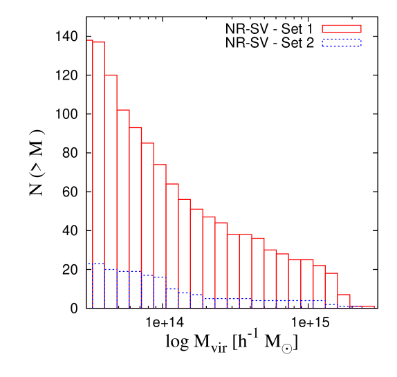
Within each Lagrangian region we increased mass resolution and added the relevant high-frequency modes of the power spectrum, following the Zoomed Initial Condition (ZIC) technique (Tormen et al., 1997). Initial conditions for hydrodynamic simulations have been generated by splitting each particle within the high–resolution region into a DM and a gas particle, having mass ratio such to reproduce the cosmic baryon fraction. Outside high–resolution regions resolution is progressively degraded, so as to save computational time, while preserving a correct description of the large–scale tidal field. We generated initial conditions at different, progressively increasing, resolution. For the hydrodynamic simulations presented here the mass of each DM particle in the high-resolution region is , with for the initial mass of gas particles. Using an iterative procedure, we have shaped each high–resolution Lagrangian region in such a way that no low–resolution particle contaminates the central “zoomed in” halo at at least out to 5 virial radii of the central cluster. This implies that each region is sufficiently large to contain more than one interesting cluster with no “contaminants” out to at least one virial radius. In total, we find clusters with , out of which about 40 have and 30 have . We show in Fig. 1 the cumulative mass distribution for this set of simulated clusters.
Simulations have been carried out using a Plummer–equivalent softening length for the computation of the gravitational force in the high–resolution region which is fixed to kpc in physical units at redshift , while being kept fixed in comoving units at higher redshift. As for the computation of hydrodynamic forces, we assume the SPH smoothing length to reach a minimum allowed value of .
Clusters from this set have been simulated using the NR-SV and CSF-M-W models. The NR-SV set is the only one simulated with GADGET 3 code.
2.2.2 Set 2
is based on 9 Lagrangian regions selected from a parent DM only cosmological box with a size of Mpc Yoshida et al. (2001). The cosmological model assumed is CDM with for the matter density, for the Hubble parameter, for the baryon density parameter and =0.9 for the normalization of the power spectrum. We refer to Dolag et al. (2009) for a more detailed description of this set of clusters. Briefly, this set includes overall 18 clusters with , out of which only 4 have . The mass distribution of these clusters is shown in Fig. 1.
Mass resolution is quite close to that of Set 1 ( and for DM and gas particles respectively), with also the same choices for the size of the gravitational softening scale and for the minimum allowed value of the SPH smoothing length. Clusters from this set have been simulated with GADGET 2 using all the seven above described different models for the description of the baryon physics.

3 Results and discussion
3.1 Mass proxies
The mass proxies that we consider in our analysis are the mass-weighted temperature , the gas mass and the product of gas mass and temperature, . All these quantities are computed within the fiducial radius , which typically corresponds to the outermost radius where scaling relations from observational data analysis are provided (e.g., Vikhlinin et al., 2009; Sun et al., 2009; Pratt et al., 2009; Maughan, 2007). With the purpose of reproducing the procedure of observational analyses we exclude the central regions, , in the computation of the temperature. The reason for this choice in the analysis of real clusters is that temperature profiles show a rather high degree of diversity in such central regions depending on their degree of “cool–coreness” (e.g., Leccardi & Molendi, 2008; Vikhlinin et al., 2006; Pratt et al., 2007). Excluding such regions suppresses the scatter in the scaling relation involving temperature (e.g., Pratt et al., 2009, and references therein). Furthermore, it places us in the regime where simulations are in closer agreement with observations (e.g., Borgani et al., 2004). The choice of the radial interval where to compute mass proxies represents our only attempt to introduce “observational effects” in our analysis. Indeed, in this paper (Paper I) we prefer to analyse in detail the intrinsic performances of the three above mass proxies, i.e. neglecting any possible observational bias which will be addressed in Paper II (Rasia et al., in prep.). We want to stress out that in this analysis i) we estimate all quantities in three-dimensions (i.e., neglecting projection effects); ii) unless otherwise stated, we use the mass–weighted definition of temperature; iii) we do not remove gas clumps at relatively low temperature when we compute both temperature and gas mass.
The simplest description of scaling relations between galaxy cluster mass and X–ray observables is that provided by the self–similar model originally proposed by (Kaiser, 1986). According to this model, the thermodynamical properties of the ICM are determined only by the action of gravity, under the assumption of virial equilibrium and spherical simmetry (e.g., Voit, 2005b, for a review). Within this model cluster total mass is the only parameter that determines all the thermodynamical properties of the hot intra–cluster gas. Accordingly, the cluster gas mass within the radius is proportional to the total mass computed within the same radius,
| (1) |
with constant of proportionality being independent of redshift. The total mass is related to the temperature according to
| (2) |
where defines the evolution of the Hubble parameter. Therefore, as defined in the paper by Kravtsov et al. (2006) the self–similar scaling of with cluster mass is given by
| (3) |
In the above relations involving ICM temperature the mass–averaged should be used, since it is more directly related to the total ICM thermal content. As such, this is the quantity relevant for the predictions of the self–similar model, rather than the spectroscopic temperature which is more affected by the complexity of the ICM thermal structure.
In the following we analyse the scaling relations for simulated clusters with masses , at five different redshifts, and . To fit the scaling relation between total mass, , and a given observable mass proxy , we use a power law
| (4) |
Following the work by Kravtsov et al. (2006) the normalization factor was fixed to , keV and keV for , and YX, respectively. We also perform the fits by fixing the slope to the self–similar value of and for , and , respectively.
The values of the slope and normalization are obtained by performing a best–fitting on the log–log relation by using the least-squares Marquardt-Levenberg algorithm (Press et al., 1992). This algorithm calculates at each iteration the sum of the squared differences with a new set of parameter values. The Marquardt-Levenberg algorithm selects the parameter values for the next iteration. The process continues until a preset criterium is met, either the fit has converged (the relative change in the residuals is less than ) or it reaches a preset iteration count limit. The intrinsic scatter in natural logarithm of the total mass, , around each best–fit scaling relation is computed as the quadratic difference between the single cluster data and the relation fitted on the whole cluster set.
3.2 Scaling relations at
In this section we will discuss the behavior of , and relations for the radiative (CSF-M-W) and non–radiative simulations (NR-SV) at for the simulated clusters of Set 1.
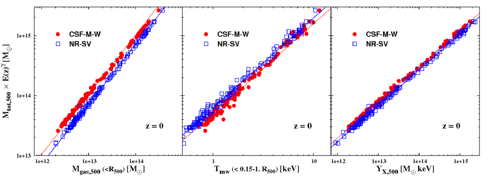
In Fig. 2 we show the relations between the total cluster mass and (left panel), (middle panel), (right panel). Besides the results of the analysis for radiative (CSF-M-W in red circles) and non–radiative (NR-SV in blue squares) simulations, we plot the best–fit relations obtained when the slope is fixed to the corresponding self-similar values, shown with the red long-dashed and the blue short-dashed lines for the CSF-M-W and NR-SV simulations, respectively.
Galaxy clusters in non–radiative simulations show a behaviour close to the self–similar one for the three studied relations. Indeed, when we consider the slope as free parameter the new best fits (not shown) over all NR-SV clusters return values consistent with , namely, for , for and , respectively. Results of the fitting relations are repoted in Tables 3.2, 3.2, and 3.2 for the , , and , respectively. The agreement with the self–similar scaling for was found also by Stanek et al. (2010) for clusters extracted from the non–radiative version of the Millenium Gas Simulations (MGS).
When radiative cooling and star formation are included in CSF-M-W simulations, the average quantities change thus modifying slope and normalization of the scaling relations. The CSF-M-W clusters (red circles in Fig. 2) deviate from the self-similar scaling relation for both and . As for the scaling, the best fit relation has a shallower slope. This is due to the fact that for radiative simulations the conversion of baryons into stars is relatively more efficient in lower mass clusters, thus corresponding to a lower mass fraction of gas left in the hot diffuse phase (e.g. Borgani et al., 2004; Kravtsov et al., 2005; Fabjan et al., 2010). As for the relation, the results for the radiative runs are characterized by a slope steeper than the self–similar one, with . In this case, the effect of including radiative physics is that of increasing the temperature of the ICM by a larger amount in less massive systems. Indeed, the more efficient cooling in lower–mass systems causes a relatively stronger adiabatic compression of gas in central core regions, as a consequence of the lack of pressure support. As a result, temperature profiles in radiative simulations of clusters are relatively steeper in less massive systems (see also Borgani et al., 2004).
| NR-SV best–fitting parameters | |||||
|---|---|---|---|---|---|
| 0.597 0.003 | 0.599 0.003 | 0.604 0.003 | 0.601 0.004 | 0.604 0.005 | |
| 14.190 0.002 | 14.188 0.002 | 14.189 0.002 | 14.177 0.003 | 14.185 0.004 | |
| 0.064 | 0.067 | 0.067 | 0.070 | 0.073 | |
| 0.107 | 0.111 | 0.111 | 0.117 | 0.122 | |
NR-SV self–similar scaling () 14.191 0.002 14.188 0.002 14.187 0.002 14.177 0.002 14.183 0.003 0.064 0.067 0.067 0.070 0.074 0.107 0.111 0.112 0.117 0.123 CSF-M-W best–fitting parameters 0.591 0.003 0.590 0.002 0.596 0.003 0.591 0.003 0.596 0.005 14.249 0.002 14.247 0.002 14.250 0.002 14.248 0.003 14.252 0.004 0.050 0.051 0.054 0.061 0.076 0.084 0.086 0.091 0.104 0.128 CSF-M-W self–similar scaling () 14.250 0.003 14.250 0.002 14.252 0.002 14.253 0.002 14.255 0.002 0.052 0.054 0.055 0.063 0.076 0.087 0.089 0.091 0.104 0.127
NR-SV self–similar scaling () 14.155 0.002 14.144 0.002 14.138 0.002 14.132 0.001 14.128 0.001 0.061 0.052 0.048 0.042 0.040 0.061 0.052 0.048 0.042 0.040 CSF-M-W best–fitting parameters 0.929 0.003 0.926 0.003 0.929 0.003 0.924 0.004 0.933 0.005 14.310 0.002 14.298 0.002 14.291 0.002 14.285 0.002 14.288 0.003 0.039 0.043 0.039 0.046 0.047 0.042 0.047 0.042 0.050 0.050 CSF-M-W self–similar scaling () 14.317 0.004 14.320 0.003 14.320 0.002 14.320 0.002 14.322 0.002 0.090 0.092 0.078 0.080 0.068 0.090 0.092 0.078 0.080 0.068
NR-SV self–similar scaling () 14.508 0.005 14.519 0.005 14.524 0.004 14.508 0.005 14.531 0.005 0.120 0.145 0.135 0.146 0.150 0.080 0.097 0.090 0.098 0.100 CSF-M-W best–fitting parameters 1.615 0.016 1.614 0.013 1.640 0.017 1.608 0.019 1.596 0.028 14.427 0.006 14.436 0.005 14.450 0.006 14.445 0.006 14.444 0.009 0.111 0.106 0.127 0.132 0.163 0.069 0.066 0.077 0.082 0.102 CSF-M-W self–similar scaling () 14.413 0.007 14.410 0.005 14.414 0.005 14.417 0.004 14.419 0.005 0.134 0.127 0.147 0.142 0.168 0.089 0.085 0.098 0.094 0.112
The deviations with respect to self–similarity that we detect in the and relations for radiative simulations are not present in the relation. In fact the best fit slope of cluster data is , close to the value of predicted by the self–similar model. As apparent from the right panel of Fig. 2, the effect of including cooling, star formation and SN feedback in the CSF-M-W runs has only a modest effect of the scaling. The reason for this is that the mass proxy provides a measure of the total thermal content of the ICM. Since this total thermal content is dominated by the mechanism of gravitational accretion of baryons within the DM–dominated potential wells of clusters, it is not surprising that the scaling of with total cluster mass very close to the self–similar prediction and that its value, at a fixed cluster mass, is weakly sensitive on the inclusion of non–radiative physics. This is even more true when we exclude central cluster regions, as we did in our analysis, which are more affected by radiative cooling.
Besides the stability of the scaling relations against variations of the ICM physics, another useful quantity to judge the robustness of mass proxies is the intrinsic scatter around the best fitting relations. In fact, the intrinsic scatter and its distribution are also an important quantities to look at when deciding which mass proxy is the best one for cosmological applications of galaxy clusters (e.g. Lima & Hu, 2005; Shaw et al., 2010). Looking at Fig. 2 we note that the mass–weighted temperature is the proxy with the largest scatter, both for CSF-M-W and NR-SV runs. To display graphically the scatter of each relation we plot in Fig. 3 the distribution of residuals, with respect to the best–fit relation, in log–mass. In all panels the distribution of the distribution of the residuals is close to a log–normal one. The intrinsic mass scatter in the residuals of the – relation is and for the CSF-M-W and NR-SV simulations, respectively (see also Table 3.2). The largest scatter is obtained for the mass–weighted temperature , reaching values of and 0.12 for non–radiative and radiative simulations, respectively, thus similar to what found by Stanek et al. (2010) for their non–radiative simulations (see also Table 3.2). As for the proxy, the intrinsic scatter in mass is and for CSF-M-W and NR-SV simulations, respectively.
Therefore, while the mass proxy is found to have a scaling with mass which is closest to the self–similar behaviour, almost independently of the inclusion of radiative physics and SN feedback, the proxy having the lowest scatter against mass is . This result is in line with that obtained by Stanek et al. (2010) from the analysis of clusters simulated with SPH, with both non–radiative physics and including cooling plus the effect of a phenomenological pre-heating. Similarly to our analysis, Stanek et al. did not attempt to include observational effects in their analysis, while they analysed scaling relations at a larger radius, instead of like in our analysis. We also note that indications for a lower scatter in the relation than in the relation have been also reported by Okabe et al. (2010) from the analysis of observational data. Their analysis was based on XMM–Newton data for the measurement of X–ray mass proxies and on weak lensing data for the measurement of total cluster masses. These results are however at variance with the original result by Kravtsov et al. (2006) who found instead to be the lowest–scatter mass proxy from their analysis of cluster simulations based on the ART adaptive-mesh refinement code. In their analysis, Kravtsov et al. showed that the residuals in the relation and in the relation anticorrelate for their radiative simulations when computed with respect to the best–fitting self–similar relation, thus justifying the smaller scatter found in the – scaling. Indeed the latter can be computed as , where is the correlation coefficient and the scatter values of temperature and gas mass (Stanek et al., 2010).
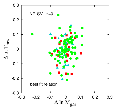
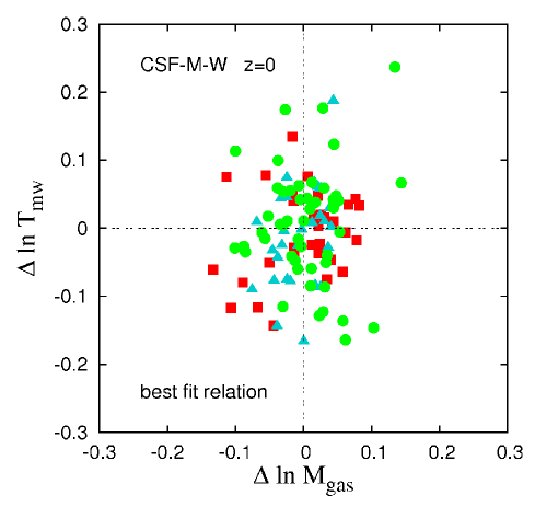
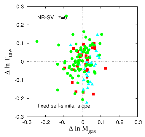
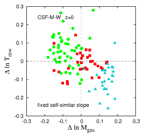
In order to look at the behaviour of such residuals in our simulations, we plot in Fig. 4 the residuals in versus the residuals in determined at fixed total mass . The residuals are computed with respect to the best–fitting relations computed without imposing the self–similar slope. Evaluating the Pearson’s correlation coefficient for the residuals we found them to be uncorrelated. We find for NR-SV distribution (left panel) and for the CSF-M-W one (right panel). The presence of a weak positive correlation explains why the scatter on is, if any, slightly larger than that on . In order to reproduce more closely the procedure followed by Kravtsov et al. (2006), we then repeated the analysis by computing the residuals with respect the best–fitting self–similar relation. The results in this case are shown in Fig. 5. As for the non–radiative runs (left panel) we find that and are again consistent with being uncorrelated for the NR-SV simulations, with . However, such scatters show a more evident sign of anti–correlation for the CSF-M-W simulations, .
In order to make more clear the reason for the anti-correlation in the residuals computed with respect to the self–similar best–fitting relation for the radiative runs, we show with different symbols in Figs. 4 and 5 the points corresponding to clusters within different mass ranges: the cyan triangles show the most massive objects with , the green points refer to groups with , while red squares represent the intermediate clusters. The only panel showing anti–correlation, the right panel of Fig. 5, also shows a clear trend with cluster mass. Anti-correlation for CSF-M-W clusters is actually a direct result of the offset of scaling relations in temperature and gas mass with respect to the expected self–similar ones. As already discussed, in the radiative runs the two relations show an opposite behaviour with respect to self-similarity: – and – are correspondinly shallower and steeper than the self–similar scaling. This means that massive clusters in CSF-M-W simulations do have higher gas masses and lower temperatures. On the other side, in low mass clusters the amount of gas is lower and temperatures are higher than expected. Therefore, in this case the presence of an anti-correlation is only a spurious effect of imposing the self–similar slopes to the best–fitting scaling relations used to compute such residuals. Clearly, in comparing our results with those by Kravtsov et al. (2006) one should remember that their analysis attempted to include observational effects in the estimate of the temperature and of the gas mass. The analysis presented here, instead, is aimed at quantifying the intrisic performances of the different mass proxies, i.e. before convolving with the effect of measuring temperature from X–ray spectra and gas mass from an projected map of X–ray surface brightness. Quite likely, including such observational effects could affect both scaling relations and the intrisinc scatter around them through the distribution of the residuals. We will address in detail these issues in a forthcoming paper (Rasia et al., in preparation).
In summary, the results presented in this section have shown that: (i) has an intrinsic scatter against cluster mass slightly smaller than , while both such proxies have a significantly lower scatter than ; (ii) is the proxy whose scaling against mass has the weakest dependence on the inclusion of radiative physics and whose slope is closest to the prediction of the self–similar model. The latter result is in line with the expectation that is a measure of the total thermal energy content of the ICM, which is mostly determined by gravitational processes once central cluster regions are excluded from the analysis. Moreover, we found that residuals in and with respect to the best–fit relations are uncorrelated independently of the adopted simulation, while anti–correlation seen in radiative simulation is as a result of the offset of and relations with respect to the expected self–similar ones.
3.3 Stability against changing ICM physics
In order to further investigate the sensitivity of the different mass proxies on the physics included in the simulation, in this section we use results from the analysis of the Set 2 simulated clusters. As already discussed in Sect. 2, this set is characterized by a much smaller number of simulated clusters than Set 1, but includes 7 different prescriptions to describe the baryonic physics.
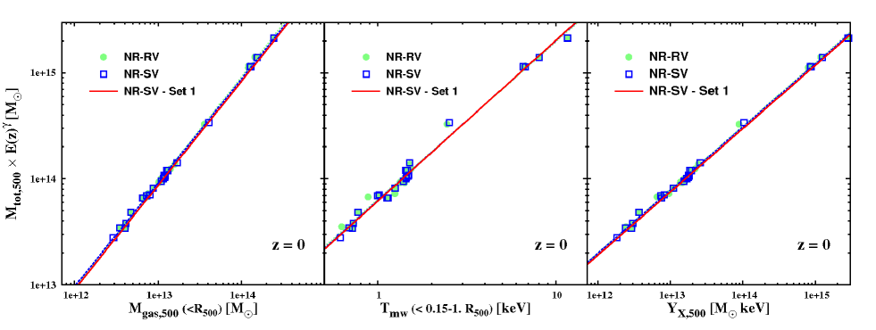
As first test we verify that simulated clusters from Set 1 and Set 2 do produce consistent results when simulated with the same physics (despite the fact they are based on somewhat different cosmological models). We show in Fig. 6 results from the non–radiative runs (NR-SV and NR-RV) of Set 2 and compare them with the best–fitting relation for the NR-SV version of Set 1 (continuous line). In performing this comparison, we should account for the different values of the baryon fraction assumed in the two simulation sets (see Sect. 2.1). To account for this, we scaled and for the Set 1 simulation NR-SV by multiplying them by the ratio of the two baryon fractions: . From this plot we note that results for the NR-SV versions of Set 1 and Set 2 agree very well with each other. Furthermore, we also note that the best fitting relations for the NR-SV and NR-RV simulations of clusters of Set 2 are also extremely similar. As shown by Dolag et al. (2005), using the time–dependent reduced viscosity scheme has the effect of increasing turbulent motions in the ICM (see also Valdarnini, 2010). Therefore, the stability of results against variations of the adopted viscosity scheme (still within SPH hydrodynamics) implies that non–thermal pressure support associated to turbulent motions have only a very modest impact on the overall gas mass and thermal content in our simulated clusters.
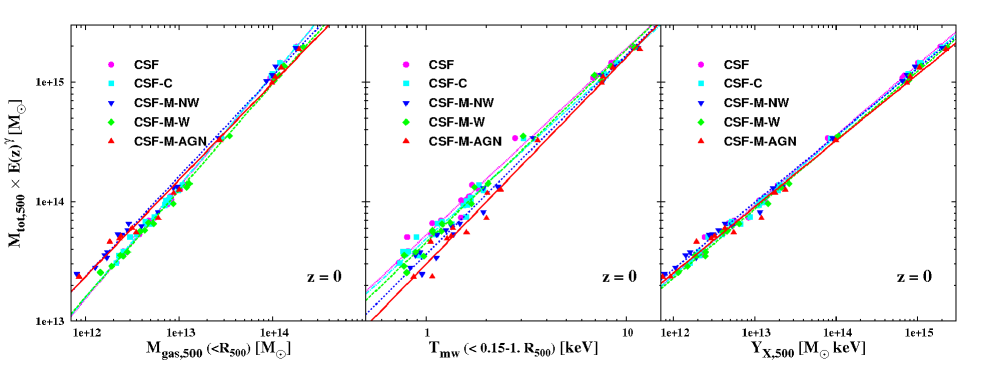
As for radiative simulations, we verified the effect of changing feedback efficiency and of including thermal conduction. All such processes are expected to change the gas distribution and the temperature structure of the ICM and, therefore, to potentially impact on the scaling relations of mass proxies against total cluster mass. We plot in Fig. 7 such scaling relations obtained the different radiative runs, CSF, CSF-C, CSF-M-NW, CSF-M-W and CSF-M-AGN along with their best–fitting relations.
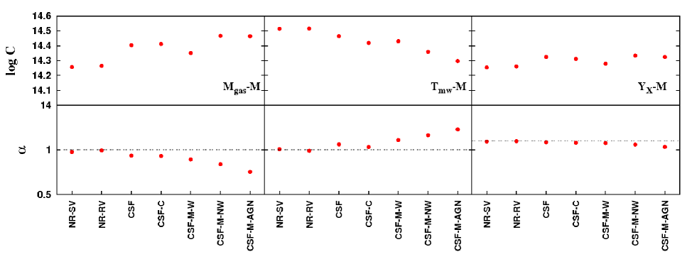
The relations involving gas mass and temperature (left and central panel, respectively) show significant dependencies on the physical processes included in the simulations, especially for relatively low mass systems. In general, while the effect of including thermal conduction is quite small, the separation between simulations with and without AGN feedback is more evident. Indeed, AGN feedback has the effect of removing a significant amount of gas from the innermost regions (e.g., Fabjan et al., 2010), thus inducing a decrease of , which is more pronounced for galaxy groups than for rich clusters. This effect can be observed in the central panel of Fig. 7, where the slope of the best fit relation for AGN simulations is of , thus significantly flatter than the self–similar scaling. The effect of AGN is not only to remove a big amount of gas from the center of galaxy groups but also to heat up the ICM in the central regions of such systems. This can be seen in the relation shown in the central panel, where the resulting slope of the relation is , again quite different from the self–similar value. Simulations including the effect of galactic winds, namely CSF, CSF-C and CSF-M-W, do have a slope closer to the self–similar one for both the () and the (–1.6) relation. The clusters simulated without feedback have an intermediate behaviour for both relations. Similarly to what already seen for simulations of Set 1, is the scaling relation characterized by the largest scatter.
On the other hand, the relation (right panel in Fig. 7) is confirmed to be the one with the weakest sensitivity on the baryon physics included in the simulation. To further emphasize the different sensitivity that different mass proxies have on the ICM physics, we plot in Fig. 8 the logarithm of the normalization, and the slope of all the best fit scaling relations for the seven different physical models simulated for the clusters of Set 2. and show the largest discrepancies in varying from to in both relation. The proxy has instead a more stable behaviour with values around . Radiative runs show also a consistent off-set from the self–similar slopes in the case of and while the slope of relation is in good agreement with the self-similar value of for all the models considered. A maximum deviation of is only present in the case of CSF-M-AGN feedback.
In summary, in this section we have shown that the mass proxy is the most robust one against changing the physical processes which determine the thermodynamical properties of the ICM and its scaling with total cluster mass has a slope which is always very close to that predicted by the self–similar model.
3.4 Evolution of scaling relations
For mass proxies to be used in cosmological applications of galaxy clusters, one has to precisely calibrate not only normalization, slope and scatter of their scaling relations with total mass for low–redshift systems, but also their evolution with redshift. Redshift evolution is especially important when considering distant clusters, located at the highest redshifts, , where they have been secured to date in statistically complete X–ray surveys. Indeed, as we approach the epoch of cluster assembly one expects clusters to be characterized by major mergers, which may significantly impact on the shaping of such scaling relations. This issue is of crucial importance if we want to constrain cosmological parameters by using upcoming and future large cluster surveys, based on the next generation of wide field X–ray telescopes (e.g., Borgani et al., 2010; Cappelluti et al., 2010).
In this Section we will address the evolution of scaling relations and of their intrinsic scatter. For an accurate study of the evolution of scaling relations we resort to the large statistical database of clusters for Set 1 simulations. All simulated clusters are analysed at five redshifts: , , , and . After measuring the normalization and slope of the scaling relations at each redshift, their redshift evolution is described through the relations:
| (5) |
Similarly to what done by Short et al. (2010), who studied the evolution of scaling relations from Millenium simulations, we take the redshift dependence of to be that predicted by the self–similar model. Therefore, we expect for a self–similar evolution of the normalization.
| – | ||||
|---|---|---|---|---|
| CSF-M-W | ||||
| NR-SV | ||||
| – | ||||
| CSF-M-W | ||||
| NR-SV | ||||
| – | ||||
| CSF-M-W | ||||
| NR-SV | ||||
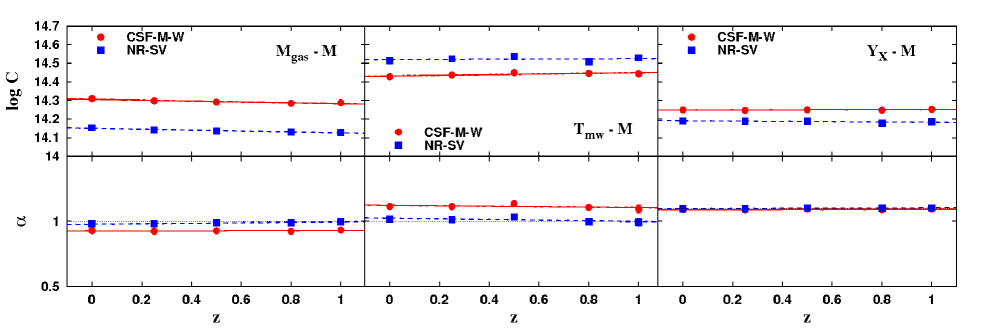
We list in Table 4 the values of the parameters which describe through eqs.5 the evolution of the scaling relations between the three mass proxies , and with the cluster total mass. Moreover, we plot in Fig. 9 the redshift dependence of normalization (after accounting for the self–similar evolution; upper panels) and slope (lower panels) of these scaling relations. The proxy has a very mild negative evolution with redshift () for both radiative and non–radiative simulations. The slope is confirmed to be very close to the self–similar value for non–radiative simulations at all redshift, with a negligible evolution of its value, while being shallower for the radiative simulations. As for the mass–weighted temperature, a slightly positive evolution is detected for the CSF simulations, while the evolution is very close to self–similar for NR simulations.
Quite interestingly, the scaling relation is the one having both the weakest sensitivity to the ICM physics at all redshifts and the smallest deviations from the self–similar predictions on the evolution of the normalization and the value of the slope. These results confirm once again the robustness of the mass proxy against variations of the physics of the ICM over the whole considered redshift range. They further confirm that, since this mass proxy provides a measure of the ICM total thermal energy content, it can be reliably described on the ground of the predictions of the self–similar model. Indeed, this model is based on the assumption that gravitational mechanisms determines the thermal content of the ICM, an assumption which is expected not to be violated by radiative and feedback processes, once we exclude core regions of galaxy clusters.
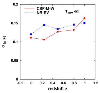
A further important aspect that characterizes the behaviour of the three analysed mass proxies at different redshifts is the evolution of their intrinsic scatter. We plot the evolution of these intrinsic scatters in Fig. 10 for both CSF (red circles) and NR (blue square) simulated clusters. The intrinsic scatter for the relation, shown in the left panel of Fig. 10, is remarkably low for both simulations, with a slight positive (negative) evolution for the radiative (non–radiative) simulations. In general, the intrinsic scatter in mass, , for varies in the narrow range per cent at all considered redshifts. CSF clusters instead show a mild decrease with a constant scatter below . Such small values are expected, since gas mass is not sensitive to cluster mergers, which are expected to play an increasingly important role at higher redshift. The middle panel of Fig. 10 shows instead the evolution of intrinsic scatter for the relation. In this case we note that the intrinsic scatter is larger and shows clear sign of a positive evolution for both radiative and non–radiative simulations, with an increase from per cent at to per cent at . The increase of the scatter in the relation agrees with the expectation that temperature is more sensitive than gas mass to the presence of substructures in the ICM, which are expected to be more prominent at high redshift, when cluster mergers are more frequent. As for the scaling relation, it has a positive evolution which is driven by the positive evolution of the scatter in the relation (right panel of Fig. 10). In general the intrinsic scatter increases from per cent at low redshift to per cent at .
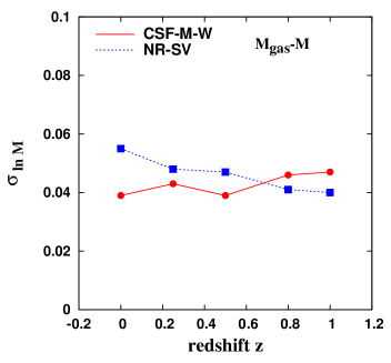
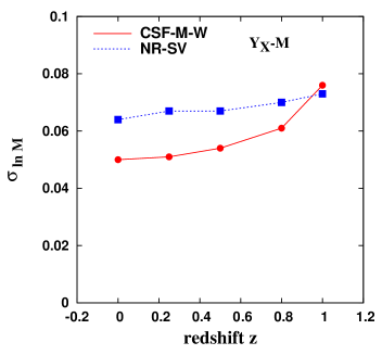
The analysis presented in this Section confirms that gas mass is the mass proxy behaving best as for the intrinsic scatter in its scaling relation with total mass, both for its value and for the stability with redshift.
An important caveat not to over interpret the results presented here concern the fact that the small values of intrinsic scatter for all mass proxies have been obtained by neglecting observational effects in the measurement of mass proxies. Such observational effects are in general expected to introduce intrinsic scatter. A typical example is provided by the presence of substructures which are not resolved in realistic observational conditions. The contribution of the X–ray emissivity from the high–density, low–temperature substructures impacts both on the estimate of the gas mass from the X–ray surface brightness profile and on the spectroscopic measurement of temperature (Mazzotta et al., 2004; Vikhlinin, 2006). In this way, observational determinations of gas mass and temperature will have a larger scatter in their scaling relation with cluster mass than their mass–weighted counterpart do.
4 Conclusions
Galaxy clusters are powerful tools for cosmological studies, since the evolution of their mass function constrain the normalization of the power spectrum, the density parameter of dark matter and dark energy as well as the dark energy equation of state, through the linear growth rate of density perturbations. When observed in the X–ray band, their high emissivity allows clusters to be detected so far out to high redshifts, . However, to fully exploit the potential of galaxy clusters as tracers of cosmic evolution, it is necessary to understand in detail the relation between mass proxies, based on easy-to-measure X–ray observables, and total cluster mass.
In this paper we focused on the study of the and mass proxies and the effect that different physical mechanisms have on the mass–observable relations. The aim of this analysis was to answer through simulations to three questions: (1) Which is the mass proxy that is least sensitive to the uncertain knowledge of the physical processes determining the thermodynamical structure of the ICM? (2) To what extent such mass proxies follow the prediction of the self–similar model for the shape of scaling relations and their redshift evolution? (3) How large is the intrinsic scatter in these scaling relations and how does it evolve with redshift?
To answer these questions we used galaxy clusters simulated with SPH using the GADGET . We combined two different sets of simulations: Set 1, composed by more than hundred clusters with mass above was used for its high statistics to calibrate scaling relations and study their scatter and redshift evolution; Set 2, containing many fewer clusters, simulated with seven different different physics schemes was instead used to study the effect of: (i) thermal conduction, (ii) artificial viscosity, (iii) cooling and star formation, (iv) galactic winds and (v) AGN feedback.
The main results of our analysis can be summarised as follows.
- (1)
-
In non–radiative simulations the relations between cluster total mass and the three considered mass proxies follow closely the self–similar prediction.
- (2)
-
In radiative simulations the and scaling relations show an opposite deviation from self–similarity. The net result is a sort of compensating effect in relation, with a nearly self–similar slope.
- (3)
-
The relation is the most stable against changing of the physical processes included in the simulations, with its slope and evolution being always very close to the predictions of the self–similar model, which is based on the assumption that gravity only drives the ICM thermodynamics. Indeed, the proxy is by definition a measure of the total thermal content of the ICM, which is dominated by the gravitational process of gas accretion.
- (4)
-
is found to be the scaling relation with the lowest scatter in mass, per cent. Moreover, the amount of scatter in this case is almost constant with redshift, independently of the simulated physics.
- (5)
-
The scatter in the relation is slightly larger that for the relation; its intrinsic scatter grows with redshift as a consequence of the increase of merging events and presence of substructure in the ICM.
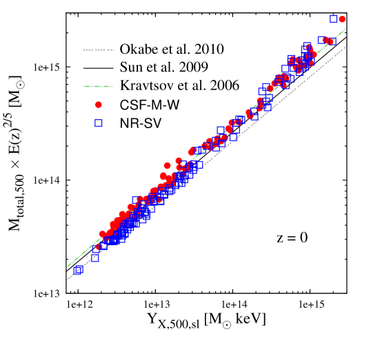
As already discussed in previous sections, the analysis discussed in this paper differs in spirit from that presented by Kravtsov et al. (2006), who instead presented results based on the inclusion of projection effects and spectroscopic estimate of the ICM temperature. In order to have a first assessment on the effect of carrying out a more observationally–oriented analysis, we also computed the mass proxy by using the spectroscopic–like definition of temperature, . To this purpose, we followed the procedure described by Vikhlinin (2006), which generalizes the analytic formula originally introduced by Mazzotta et al. (2004), to include relatively cold clusters with temperature below 3 keV. 333We use the algorithm proposed by Vikhlinin (2006) that resorts to precomputed tables of some parameters for the observed spectra as a function of the temperature. Tables were generated with the code that is publicly available at http://hea-www.harvard.edu/ alexey/mixT. The tables were created by fixing for the galactic hydrogen column density, solar abundances to the values by Grevesse & Sauval (1998), the Chandra ACIS-S CCD response function and the photon energy range to keV. We plot in Fig. 11 the scaling relation between total mass and for the radiative and non–radiative versions of the clusters of Set 1. As expected the scatter in this case is larger than when adopting the mass-weighted definition of temperature: it increases from to and from to for the NR-SV and CSF-M-W simulations, respectively. Moreover also a slight deviation from self–similarity is observed for non–radiative runs, with , while the slope for radiative runs, , agrees with the self–similar value. In the same figure we also compare our results with those presented in literature, both from simulations (Kravtsov et al., 2006) and from observational data (Sun et al., 2009; Okabe et al., 2010). Our results are in a good agreement although some discrepancy is seen at the high mass end of clusters and for NR-SV galaxy groups.
Clearly, a more detailed analysis of how observational effects will affect the scaling relations measured from our simulated cluster sets requires using a dedicated software, like X–ray Map Simulator (X–MAS; e.g. Gardini et al., 2004; Rasia et al., 2005, 2008), to extract mock images and spectra from simulations and to reduce data using the same procedure followed for observational data (Rasia et al., in prep., Paper II).
Acknowledgements
We are greatly indebted to Volker Springel for providing us with the non–public version of GADGET . We acknowledge useful discussions with Gus Evrard, Andrey Kravtsov and Chris Miller. This work has been partially supported by PRIN-MIUR grant “The Cosmic Cycle of Baryons” and PRIN-INAF 2009 grant “Towards an italian network for computational cosmology”, by ASI–AAE and ASI–COFIS grants and by the INFN–PD51 grant. DF acknowledges the support by the European Union and Ministry of Higher Education, Science and Technology of Slovenia. ER acknowledges the Michigan Society of Fellow. KD acknowledges the financial support by the “HPC-Europa Transnational Access program” and the hospitality of CINECA and of the Department of Physics of the University of Trieste. KD also acknowledges the support by the DFG Priority Programme 1177 and additional support by the DFG Cluster of Excellence ”Origin and Structure of the Universe”. DF, SB and ER acknowledge the hospitality of the Sesto Center for Astrophysics (SCfA), where part of the work has been carried out. Simulations have been carried out at the CINECA Supercomputing Center (Bologna), with CPU time assigned thanks to an INAF–CINECA grant and to an agreement between CINECA and the University of Trieste.
References
- Ameglio et al. (2009) Ameglio S., Borgani S., Pierpaoli E., Dolag K., Ettori S., Morandi A., 2009, MNRAS, 394, 479
- Arnaud et al. (2009) Arnaud M., Pratt G. W., Piffaretti R., Boehringer H., Croston J. H., Pointecouteau E., 2009, ArXiv e-prints
- Balsara (1995) Balsara D. S., 1995, Journal of Computational Physics, 121, 357
- Bartelmann & Steinmetz (1996) Bartelmann M., Steinmetz M., 1996, MNRAS, 283, 431
- Borgani & Kravtsov (2009) Borgani S., Kravtsov A., 2009, ArXiv e-prints, ASL, in press
- Borgani et al. (2004) Borgani S., Murante G., Springel V., Diaferio A., Dolag K., Moscardini L., Tormen G., Tornatore L., Tozzi P., 2004, MNRAS, 348, 1078
- Borgani et al. (2010) Borgani S., Rosati P., Sartoris B., Tozzi P., Giacconi R., 2010, ArXiv e-prints
- Borgani et al. (2001) Borgani S., Rosati P., Tozzi P., Stanford S. A., Eisenhardt P. R., Lidman C., Holden B., Della Ceca R., Norman C., Squires G., 2001, ApJ, 561, 13
- Burns et al. (2008) Burns J. O., Hallman E. J., Gantner B., Motl P. M., Norman M. L., 2008, ApJ, 675, 1125
- Cappelluti et al. (2010) Cappelluti N., Predehl P., Boehringer H., Brunner H., Brusa M., Burwitz V., et al. 2010, ArXiv e-prints
- Croston et al. (2008) Croston J. H., Pratt G. W., Böhringer H., Arnaud M., Pointecouteau E., Ponman T. J., Sanderson A. J. R., Temple R. F., Bower R. G., Donahue M., 2008, A&A, 487, 431
- Dolag et al. (2009) Dolag K., Borgani S., Murante G., Springel V., 2009, MNRAS, 399, 497
- Dolag et al. (2004) Dolag K., Jubelgas M., Springel V., Borgani S., Rasia E., 2004, ApJL, 606, L97
- Dolag et al. (2005) Dolag K., Vazza F., Brunetti G., Tormen G., 2005, MNRAS, 364, 753
- Eke et al. (1996) Eke V. R., Cole S., Frenk C. S., 1996, MNRAS, 282, 263
- Ettori et al. (2006) Ettori S., Dolag K., Borgani S., Murante G., 2006, MNRAS, 365, 1021
- Ettori et al. (2004) Ettori S., Tozzi P., Borgani S., Rosati P., 2004, A&A, 417, 13
- Evrard et al. (1996) Evrard A. E., Metzler C. A., Navarro J. F., 1996, ApJ, 469, 494
- Fabjan et al. (2010) Fabjan D., Borgani S., Tornatore L., Saro A., Murante G., Dolag K., 2010, MNRAS, 401, 1670
- Gardini et al. (2004) Gardini A., Rasia E., Mazzotta P., Tormen G., De Grandi S., Moscardini L., 2004, MNRAS, 351, 505
- Gottloeber et al. (2006) Gottloeber S., Yepes G., Wagner C., Sevilla R., 2006, ArXiv Astrophysics e-prints
- Grevesse & Sauval (1998) Grevesse N., Sauval A. J., 1998, Space Science Reviews, 85, 161
- Haardt & Madau (1996) Haardt F., Madau P., 1996, ApJ, 461, 20
- Hartley et al. (2008) Hartley W. G., Gazzola L., Pearce F. R., Kay S. T., Thomas P. A., 2008, MNRAS, 386, 2015
- Henry & Arnaud (1991) Henry J. P., Arnaud K. A., 1991, ApJ, 372, 410
- Henry et al. (2009) Henry J. P., Evrard A. E., Hoekstra H., Babul A., Mahdavi A., 2009, ApJ, 691, 1307
- Ikebe et al. (2002) Ikebe Y., Reiprich T. H., Böhringer H., Tanaka Y., Kitayama T., 2002, A&A, 383, 773
- Jeltema et al. (2008) Jeltema T. E., Hallman E. J., Burns J. O., Motl P. M., 2008, ApJ, 681, 167
- Jubelgas et al. (2004) Jubelgas M., Springel V., Dolag K., 2004, MNRAS, 351, 423
- Kaiser (1986) Kaiser N., 1986, MNRAS, 222, 323
- Kay et al. (2007) Kay S. T., da Silva A. C., Aghanim N., Blanchard A., Liddle A. R., Puget J.-L., Sadat R., Thomas P. A., 2007, MNRAS, 377, 317
- Komatsu et al. (2010) Komatsu E., Smith K. M., Dunkley J., Bennett C. L., Gold B., Hinshaw G., et al. 2010, ArXiv e-prints
- Kravtsov et al. (2005) Kravtsov A. V., Nagai D., Vikhlinin A. A., 2005, ApJ, 625, 588
- Kravtsov et al. (2006) Kravtsov A. V., Vikhlinin A., Nagai D., 2006, ApJ, 650, 128
- Lau et al. (2009) Lau E. T., Kravtsov A. V., Nagai D., 2009, ApJ, 705, 1129
- Leccardi & Molendi (2008) Leccardi A., Molendi S., 2008, A&A, 486, 359
- Lima & Hu (2005) Lima M., Hu W., 2005, Phys. Rev. D, 72, 043006
- Loken et al. (2002) Loken C., Norman M. L., Nelson E., Burns J., Bryan G. L., Motl P., 2002, ApJ, 579, 571
- Mahdavi et al. (2008) Mahdavi A., Hoekstra H., Babul A., Henry J. P., 2008, MNRAS, 384, 1567
- Mantz et al. (2010) Mantz A., Allen S. W., Ebeling H., Rapetti D., Drlica-Wagner A., 2010, MNRAS, pp 1030–+
- Markevitch (1998) Markevitch M., 1998, ApJ, 504, 27
- Maughan (2007) Maughan B. J., 2007, ApJ, 668, 772
- Mazzotta et al. (2004) Mazzotta P., Rasia E., Moscardini L., Tormen G., 2004, MNRAS, 354, 10
- Monaghan (1997) Monaghan J. J., 1997, Journal of Computational Physics, 136, 298
- Morris & Monaghan (1997) Morris J. P., Monaghan J. J., 1997, Journal of Computational Physics, 136, 41
- Muanwong et al. (2006) Muanwong O., Kay S. T., Thomas P. A., 2006, ApJ, 649, 640
- Nagai et al. (2007) Nagai D., Kravtsov A. V., Vikhlinin A., 2007, ApJ, 668, 1
- Nagai et al. (2007) Nagai D., Vikhlinin A., Kravtsov A. V., 2007, ApJ, 655, 98
- O’Hara et al. (2006) O’Hara T. B., Mohr J. J., Bialek J. J., Evrard A. E., 2006, ApJ, 639, 64
- Okabe et al. (2010) Okabe N., Zhang Y., Finoguenov A., Takada M., Smith G. P., Umetsu K., Futamase T., 2010, ArXiv e-prints
- Padovani & Matteucci (1993) Padovani P., Matteucci F., 1993, ApJ, 416, 26
- Pierpaoli et al. (2003) Pierpaoli E., Borgani S., Scott D., White M., 2003, MNRAS, 342, 163
- Piffaretti et al. (2010) Piffaretti R., Arnaud M., Pratt G. W., Pointecouteau E., Melin J., 2010, ArXiv e-prints
- Poole et al. (2007) Poole G. B., Babul A., McCarthy I. G., Fardal M. A., Bildfell C. J., Quinn T., Mahdavi A., 2007, MNRAS, 380, 437
- Pratt et al. (2007) Pratt G. W., Böhringer H., Croston J. H., Arnaud M., Borgani S., Finoguenov A., Temple R. F., 2007, A&A, 461, 71
- Pratt et al. (2009) Pratt G. W., Croston J. H., Arnaud M., Böhringer H., 2009, A&A, 498, 361
- Press et al. (1992) Press W. H., Teukolsky S. A., Vetterling W. T., Flannery B. P., 1992, Numerical recipes in C. The art of scientific computing
- Puchwein et al. (2008) Puchwein E., Sijacki D., Springel V., 2008, ApJL, 687, L53
- Rasia et al. (2005) Rasia E., Mazzotta P., Borgani S., Moscardini L., Dolag K., Tormen G., Diaferio A., Murante G., 2005, ApJL, 618, L1
- Rasia et al. (2008) Rasia E., Mazzotta P., Bourdin H., Borgani S., Tornatore L., Ettori S., Dolag K., Moscardini L., 2008, ApJ, 674, 728
- Rasia et al. (2004) Rasia E., Tormen G., Moscardini L., 2004, MNRAS, 351, 237
- Reiprich & Böhringer (2002) Reiprich T., Böhringer H., 2002, ApJ, 567, 716
- Roncarelli et al. (2006) Roncarelli M., Ettori S., Dolag K., Moscardini L., Borgani S., Murante G., 2006, MNRAS, 373, 1339
- Salpeter (1955) Salpeter E. E., 1955, ApJ, 121, 161
- Schuecker et al. (2002) Schuecker P., Guzzo L., Collins C. A., Böhringer H., 2002, MNRAS, 335, 807
- Shaw et al. (2010) Shaw L. D., Holder G. P., Dudley J., 2010, ApJ, 716, 281
- Short et al. (2010) Short C. J., Thomas P. A., Young O. E., Pearce F. R., Jenkins A., Muanwong O., 2010, ArXiv e-prints
- Sijacki & Springel (2006) Sijacki D., Springel V., 2006, MNRAS, 366, 397
- Springel (2005) Springel V., 2005, MNRAS, 364, 1105
- Springel et al. (2005) Springel V., Di Matteo T., Hernquist L., 2005, MNRAS, 361, 776
- Springel & Hernquist (2003) Springel V., Hernquist L., 2003, MNRAS, 339, 289
- Stanek et al. (2010) Stanek R., Rasia E., Evrard A. E., Pearce F., Gazzola L., 2010, ApJ, 715, 1508
- Steinmetz (1996) Steinmetz M., 1996, MNRAS, 278, 1005
- Sun et al. (2009) Sun M., Voit G. M., Donahue M., Jones C., Forman W., Vikhlinin A., 2009, ApJ, 693, 1142
- Sutherland & Dopita (1993) Sutherland R. S., Dopita M. A., 1993, ApJS, 88, 253
- Tormen et al. (1997) Tormen G., Bouchet F. R., White S. D. M., 1997, MNRAS, 286, 865
- Tornatore et al. (2007) Tornatore L., Borgani S., Dolag K., Matteucci F., 2007, MNRAS, 382, 1050
- Valdarnini (2010) Valdarnini R., 2010, ArXiv e-prints
- Vikhlinin (2006) Vikhlinin A., 2006, ApJ, 640, 710
- Vikhlinin et al. (2009) Vikhlinin A., Burenin R. A., Ebeling H., Forman W. R., Hornstrup A., Jones C., Kravtsov A. V., Murray S. S., Nagai D., Quintana H., Voevodkin A., 2009, ApJ, 692, 1033
- Vikhlinin et al. (2006) Vikhlinin A., Kravtsov A., Forman W., Jones C., Markevitch M., Murray S. S., Van Speybroeck L., 2006, ApJ, 640, 691
- Vikhlinin et al. (2009) Vikhlinin A., Kravtsov A. V., Burenin R. A., Ebeling H., Forman W. R., Hornstrup A., Jones C., Murray S. S., Nagai D., Quintana H., Voevodkin A., 2009, ApJ, 692, 1060
- Vikhlinin et al. (2003) Vikhlinin A., Voevodkin A., Mullis C. R., VanSpeybroeck L., Quintana H., McNamara B. R., Gioia I., Hornstrup A., Henry J. P., Forman W. R., Jones C., 2003, ApJ, 590, 15
- Voevodkin & Vikhlinin (2004) Voevodkin A., Vikhlinin A., 2004, ApJ, 601, 610
- Voit (2005a) Voit G. M., 2005a, Advances in Space Research, 36, 701
- Voit (2005b) Voit G. M., 2005b, Reviews of Modern Physics, 77, 207
- Yang et al. (2009) Yang H., Ricker P. M., Sutter P. M., 2009, ApJ, 699, 315
- Yoshida et al. (2001) Yoshida N., Sheth R. K., Diaferio A., 2001, MNRAS, 328, 669
- Zhang et al. (2010) Zhang Y., Okabe N., Finoguenov A., Smith G. P., Piffaretti R., Valdarnini R., Babul A., Evrard A. E., Mazzotta P., Sanderson A. J. R., Marrone D. P., 2010, ApJ, 711, 1033