Dual-Tree Fast Gauss Transforms

Abstract

Kernel density estimation (KDE) is a popular statistical technique for estimating the underlying density distribution with minimal assumptions. Although they can be shown to achieve asymptotic estimation optimality for any input distribution, cross-validating for an optimal parameter requires significant computation dominated by kernel summations. In this paper we present an improvement to the dual-tree algorithm, the first practical kernel summation algorithm for general dimension. Our extension is based on the series-expansion for the Gaussian kernel used by fast Gauss transform. First, we derive two additional analytical machinery for extending the original algorithm to utilize a hierarchical data structure, demonstrating the first truly hierarchical fast Gauss transform. Second, we show how to integrate the series-expansion approximation within the dual-tree approach to compute kernel summations with a user-controllable relative error bound. We evaluate our algorithm on real-world datasets in the context of optimal bandwidth selection in kernel density estimation. Our results demonstrate that our new algorithm is the only one that guarantees a hard relative error bound and offers fast performance across a wide range of bandwidths evaluated in cross validation procedures.

1 Introduction

Kernel density estimation (KDE) is the most widely used and studied nonparametric density estimation method. The model is the reference dataset $\mathcal{R}$ itself, containing the reference points indexed by natural numbers. Assume a local kernel function $K_{h}(\cdot)$ centered upon each reference point, and its scale parameter $h$ (the ’bandwidth’). The common choices for $K_{h}(\cdot)$ include the spherical, Gaussian and Epanechnikov kernels. We are given the query dataset $\mathcal{Q}$ containing query points whose densities we want to predict. The density estimate at the $i$-th query point $q_{i}\in\mathcal{Q}$ is:

$$\hat{p}_{h}(q_{i})=\frac{1}{|\mathcal{R}|}\sum\limits_{r_{j}\in\mathcal{R}}\frac{1}{V_{Dh}}K_{h}\left(||q_{i}-r_{j}||\right)$$ (1)

where $||q_{i}-r_{j}||$ denotes the Euclidean distance between the $i$-th query point $q_{i}$ and the $j$-th reference point $r_{j}$, $D$ the dimensionality of the data, $|\mathcal{R}|$ the size of the reference dataset, and $V_{Dh}=\int\limits_{-\infty}^{\infty}K_{h}(z)dz$, a normalizing constant depending on $D$ and $h$. With no assumptions on the true underlying distribution, if $h\rightarrow 0$ and $|\mathcal{R}|h\rightarrow\infty$ and $K(\cdot)$ satisfy some mild conditions:

$$\int|\hat{p}_{h}(x)-p(x)|dx\rightarrow 0$$ (2)

as $|\mathcal{R}|\rightarrow\infty$ with probability 1. As more data are observed, the estimate converges to the true density.

Algorithm 1 $\mbox{{NaiveKDE}}(\mathcal{Q},\mathcal{R})$: A brute-force computation of KDE.

  for each $q_{i}\in\mathcal{Q}$ do

     $G(q_{i},\mathcal{R})\leftarrow 0$

     for each $r_{j}\in\mathcal{R}$ do

        $G(q_{i},\mathcal{R})\leftarrow G(q_{i},\mathcal{R})+K_{h}(||q_{i}-r_{j}||)$

     Normalize each $G(q_{i},\mathcal{R})$

In order to build our model for evaluating the densities at each $q_{i}\in\mathcal{Q}$, we need to find the initially unknown asymptotically optimal bandwidth $h^{*}$ for the given reference dataset $\mathcal{R}$. There are two main types of cross-validation methods for selecting the asymptotically optimal bandwidth. Cross-validation methods use the reference dataset $\mathcal{R}$ as the query dataset $\mathcal{Q}$ (i.e. $\mathcal{Q}=\mathcal{R}$). Likelihood cross-validation is derived by minimizing the Kullback-Leibler divergence $\int p(x)\log\frac{p(x)}{\hat{p}_{h}(x)}dx$, which yields the score:

$$CV_{LK}(h)=\frac{1}{|\mathcal{R}|}\sum\limits_{r_{j}\in\mathcal{R}}\log\hat{p}_{h,-j}(r_{j})$$ (3)

where the $-j$ subscript denotes an estimate using all $|\mathcal{R}|$ points except the $j$-th reference point. The bandwidth $h^{*}_{CV_{LK}}$ that maximizes $CV_{LK}(h)$ is an asymptotically optimal bandwidth in likelihood cross validation sense. Least-squares cross-validation minimizes the integrated squared error
$\int\left(\hat{p}_{h}(x)-p(x)\right)^{2}dx$, yielding the score:

$$CV_{LS}(h)=\frac{1}{|\mathcal{R}|}\sum\limits_{r_{j}\in\mathcal{R}}\left(\hat{p}^{*}_{-j}(r_{j})-2\hat{p}_{-j}(r_{j})\right)$$ (4)

where $\hat{p}^{*}_{-j}(\cdot)$ is evaluated using the convolution kernel $K_{h}(\cdot)*K_{h}(\cdot)$. For the Gaussian kernel with bandwidth of $h$, the convolution kernel $K_{h}(\cdot)*K_{h}(\cdot)$ is the Gaussian kernel with bandwidth of $2h$. Both cross validation scores require $|\mathcal{R}|$ density estimate based on $|\mathcal{R}|-1$ points, yielding a brute-force computational cost scaling quadratically (that is $O(|\mathcal{R}|^{2})$) (see Algorithm 1). To make matters worse, nonparametric methods require a large number of reference points for convergence to the true underlying distribution and this has prevented many practitioners from applying nonparametric methods for function estimation.

1.1 Efficient Computation of Gaussian Kernel Sums

One of the most commonly used kernel function is the Gaussian kernel, $K_{h}(||q_{i}-r_{j}||)=e^{\frac{-||q_{i}-r_{j}||^{2}}{2h^{2}}}$, although it is not the asymptotically optimal kernel. In this paper we focus on evaluating the Gaussian sums efficiently for each $q_{i}\in\mathcal{Q}$:

$$G(q_{i},\mathcal{R})=\sum\limits_{r_{j}\in\mathcal{R}}e^{\frac{-||q_{i}-r_{j}||^{2}}{2h^{2}}}$$ (5)

which is proportional to $\hat{p}(q_{i})$ using the Gaussian kernel. This computationally expensive sum is evaluated many times when cross-validating for an asymptotically optimal bandwidth for the Gaussian kernel. Algorithms have been developed to approximate the Gaussian kernel sums at the expense of reduced precision. We consider the following two error bound criteria that measure the quality of the approximation with respect to the true value.

Definition 1.1.

(Bounding the absolute error) An approximation algorithm guarantees $\epsilon$ absolute error bound, if for each exact value $\Phi(q_{i},\mathcal{R})$, it computes an approximation $\widetilde{\Phi}(q_{i},\mathcal{R})$ such that $|\widetilde{\Phi}(q_{i},\mathcal{R})-\Phi(q_{i},\mathcal{R})|\leq\epsilon$.

Definition 1.2.

(Bounding the relative error) An approximation algorithm guarantees $\epsilon$ relative error bound, if for each exact value $\Phi(q_{i},\mathcal{R})$, it computes an approximation $\widetilde{\Phi}(x_{q},\mathcal{R})$ such that $|\widetilde{\Phi}(q_{i},\mathcal{R})-\Phi(q_{i},\mathcal{R})|\leq\epsilon|\Phi(q_{i},\mathcal{R})|$.

Bounding the relative error is much harder because the error bound is in terms of the initially unknown exact quantity. Many previous methods [11, 19] have focused on bounding the absolute error. Nevertheless, the relative error bound criterion is preferred to the absolute error bound criterion in statistical applications. Therefore, our experiment will evaluate the performance of the algorithms for achieving the user-specified relative error tolerance. Our new algorithm which builds upon [9, 6, 7] is the only one to guarantee both the absolute error and the relative error bound criterion for all density estimates.

1.2 Previous Approaches

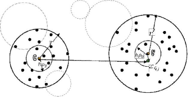
Figure 1: (a) Grid structure used in fast Gauss transform and multidimensional fast Fourier transform. (b) Single-level Clustering structure used in improved fast Gauss transform.

There are three main approaches proposed for overcoming the computational barrier in evaluating the Gaussian kernel sums:

1. to expand the kernel sum as a power series [11, 19, 13] using a grid or a flat-clustering.

2. to express the kernel sum as a convolution sum by using the grid of field charges created from the dataset [18].

3. to utilize an adaptive hierarchical structure to group data points based on proximity [9, 6, 7].

Now we briefly describe the strengths and the weaknesses of these methods.

The Fast Gauss Transform (FGT). FGT [11] belongs to a family of methods called the Fast Multipole Methods (FMM). These family of methods come with rigorous error bound on the kernel sums. Unlike other FMM algorithms, FGT uses a grid structure (see Figure 1) whose maximum side length is restricted to be at most the bandwidth $h$ used in cross-validation due to the error bound criterion. FGT has not been widely used in higher dimensional statistical contexts. First, the number of the terms in the power series expansion for the kernel sums grows exponentially with dimensionality $D$; this causes computational bottleneck in evaluating the series expansion or translating a series expansion from one center to another. Second, the grid structure is extremely inefficient in higher dimensions since the storage cost is exponential in $D$ and many of the boxes will be empty.

The Improved Fast Gauss Transform (IFGT). IFGT is similar to FMM but utilizes a flat clustering to group data points (see Figure 1), which is more efficient than a grid structure used in FGT. The number of clusters $k$ is chosen in advance. A partition of the data points into $C_{1}$, $C_{2}$, $\cdots$, $C_{k}$ is formed so that each reference point $r_{j}\in\mathcal{R}$ is grouped according to its proximity to the set of representative points $c_{1}$, $c_{2}$, $\cdots$, $c_{k}$. That is, $r_{j}\in C_{m}$ (whose representative point is $c_{m}$) if and only if $||r_{j}-c_{m}||\leq||r_{j}-c_{l}||$ for $1\leq l\leq k$.

Furthermore, IFGT proposes using a different series expansion that does not require translation of expansion centers as done in FGT. The original algorithm [19] required tweaking of multiple parameters which did not offer for a user to control the accuracy of the approximation. The latest version [13] is now fully automatic in choosing the approximation parameter for the absolute error bound, but is still inefficient except on large bandwidth parameters. We will discuss this further in Section 4.

(a) Nearest Neighbor Binning Rule $(A=1,B=C=D=0)$

(b) Linear Binning Rule $(A=\frac{4}{9},B=\frac{2}{9},C=\frac{1}{9},D=\frac{2}{9})$

Figure 2: Two possible binning rules for KDE using multidimensional fast Fourier transform. Consider a data point falling in a two-dimensional rectangle. In 2(a), the entire weight is assigned to the nearest grid point. In 2(b), the weight is distributed to all neighboring grid points by linear interpolation.

Fast Fourier Transform (FFT). FFT is often quoted as the solution to the computational problem in evaluating the Gaussian kernel sums. Gaussian kernel summation using FFT is described in [14] and  [18].  [14] discusses the implementation of KDE only in a univariate case, while [18] extends [14] to handle more than one dimension. It uses a grid structure shown in Figure 1 by specifying the number of grid points along each dimension.

The algorithm first computes the $M_{1}\times\cdot\cdot\cdot\times M_{D}$ matrix by binning the data assigning the raw data to neighboring grid points using one of the binning rules. This involves computing the minimum and maximum coordinate values ($g_{i,M_{i}},g_{i,1}$), and the grid width $\delta_{i}=\frac{g_{i,M_{i}}-g_{i,1}}{M_{i}-1}$ for each $i$-th dimension. This essentially divides each $i$-th dimension into $M_{i}-1$ intervals of equal length. In particular, [18] discusses two different types of binning rules - linear binning, which is recommended by Silverman, and nearest-neighbor binning. [18] states that nearest-neighbor binning rule performs poorly, so we will test the implementation using the linear binning rule, as recommended by both authors. In addition, we compute the $L_{1}\times\cdot\cdot\cdot\times L_{D}$ kernel weight matrix, where $L_{i}=\min\left(\left\lfloor\frac{\tau h}{\delta_{i}}\right\rfloor,M_{i}-1\right)$, with $\tau\approx 4$ and $K_{l}=\prod\limits_{k=1}^{d}e^{\frac{-0.5l_{k}\delta_{k}}{h^{2}}}$, $-L_{k}\leq l_{k}\leq L_{k}$, for $l=[l_{1},...,l_{D}]^{T}\in\mathbb{Z}^{D}$.

To reduce the wrap-around effects of fast Fourier transform near the dataset boundary, we appropriately zero-pad the grid count and the kernel weight matrices to two matrices of the dimensionality $P_{1}\times\cdot\cdot\cdot P_{D}$, where $P_{i}=2^{\log_{2}\lceil M_{i}+L_{i}\rceil}$. The key ingredient in this method is the use of Convolution Theorem for Fourier transforms. The structure of the computed grid count matrix and the kernel weight matrix is crafted to take advantage of the fast Fourier transform. For every grid point $g=(g_{1j_{1}},...,g_{dj_{D}})$, $\tilde{s_{k}}(g_{j})=\sum\limits_{l_{1}=-L_{1}}^{L_{1}}\cdots\sum\limits_{l_{D}=-L_{D}}^{L_{D}}c_{j-l}K_{k,l}$ can be computed using the Convolution Theorem for Fourier Transform. After taking the convolution of the grid count matrix and the kernel weight matrix, the $M_{1}\times\cdots\times M_{D}$ sub-matrix in the upper left corner of the resultant matrix contains the kernel density estimate of the grid points. The density estimate of each query point is then linearly interpolated using the density estimates of neighboring grid points inside the cell it falls into.

The grid count matrix: $c^{Z}=\begin{pmatrix}c_{1,1}&\cdots&c_{1,M_{2}}\\ \vdots&\ddots&\vdots&\textbf{0}\\ c_{M_{1},1}&\cdots&c_{M_{1},M_{2}}\\ &\textbf{0}&&\textbf{0}\end{pmatrix}$

The kernel weight matrix: $\textbf{K}^{Z}=\begin{pmatrix}K_{00}&\cdots&K_{0L_{2}}&&K_{0L_{2}}&\cdots&K_{01}\\ \vdots&\ddots&\vdots&\textbf{0}&\vdots&\ddots&\vdots\\ K_{L_{1}0}&\cdots&K_{L_{1}L_{2}}&&K_{L_{1}L_{2}}&\cdots&K_{L_{1}1}\\ &\textbf{0}&&\textbf{0}&&\textbf{0}\\ K_{L_{1}0}&\cdots&K_{L_{1}L_{2}}&&K_{L_{1}L_{2}}&\cdots&K_{L_{1}1}\\ \vdots&\ddots&\vdots&\textbf{0}&\vdots&\ddots&\vdots\\ K_{10}&\cdots&K_{1L_{2}}&&K_{1L_{2}}&\cdots&K_{11}\end{pmatrix}$

where $K_{l_{1},l_{2}}=e^{\frac{-0.5((l_{1}\delta_{1})^{2}+(l_{2}\delta_{2})^{2})}{h^{2}}}$.

Figure 3: The grid count and the kernel weight matrix formed for a two-dimensional dataset. They are formed by appropriately zero-padding for taking the boundary-effects of fast Fourier transform based algorithms into account.

However, performing a calculation on equally-spaced grid points introduces artifacts at the boundaries of the data. The linear interpolation of the data points by assigning to neighboring grid points introduce further errors. Increasing the number of grid points to use along each dimension can provide more accuracy but also require more space to store the grid. Moreover, it is impossible to directly quantify incurred error on each estimate in terms of the number of grid points.

Dual-tree KDE. In terms of discrete algorithmic structure, the dual-tree framework of [8] generalizes all of the well-known kernel summation algorithms. These include the Barnes-Hut algorithm [2], the Fast Multipole Method [10], Appel’s algorithm [1], and the WSPD [5]: the dual-tree method is a node-node algorithm (considers query regions rather than points), is fully recursive, can use distribution-sensitive data structures such as kd-trees, and is bichromatic (can specialize for differing query set $\mathcal{Q}$ and reference set $\mathcal{R}$). It was applied to the problem of kernel density estimation in [9] using a simple variant of a centroid approximation used in [1].

This algorithm is currently the fastest Gaussian kernel summation algorithm for general dimensions. Unfortunately, when performing cross-validation to determine the (initially unknown) optimal bandwidth, both sub-optimally small and large bandwidths must be evaluated. Section 4 demonstrates that the dual-tree method tends to be efficient at the optimal bandwidth and at bandwidths below the optimal bandwidth and at very large bandwidths. However, its performance degrades for intermediately large bandwidths.

1.3 Our Contribution

In this paper we present an improvement to the dual-tree algorithm [9, 6, 7], the first practical kernel summation algorithm for general dimension. Our extension is based on the series-expansion for the Gaussian kernel used by fast Gauss transform [11]. First, we derive two additional analytical machinery for extending the original algorithm to utilize a adaptive hierarchical data structure called $kd$-trees [4], demonstrating the first truly hierarchical fast Gauss transform, which we call the Dual-tree Fast Gauss Transform (DFGT). Second, we show how to integrate the series-expansion approximation within the dual-tree approach to compute kernel summations with a user-controllable relative error bound. We evaluate our algorithm on real-world datasets in the context of optimal bandwidth selection in kernel density estimation. Our results demonstrate that our new algorithm is the only one that guarantees a relative error bound and offers fast performance across a wide range of bandwidths evaluated in cross validation procedures.

1.4 Structure of This Paper

This paper builds on [12] where the Dual-Tree Fast Gauss Transform was presented briefly. It adds details on the approximation mechanisms used in the algorithm and provides a more thorough comparison with the other algorithms. In Section 2, we introduce a general computational strategy for efficiently computing the Gaussian kernel sums. In Section 3, we describe our extensions to the dual-tree algorithm to handle higher-order series expansion approximations. In Section 4, we provide performance comparison with some of the existing methods for evaluating the Gaussian kernel sums.

1.5 Notations

The general notation conventions used throughout this paper are as follows. $\mathcal{Q}$ denotes the set of query points for which we want to make the density computations. $\mathcal{R}$ denotes the set of reference points which are used to construct the kernel density estimation model. Query points and reference points are indexed by natural numbers $i,j\in\mathbb{N}$ and denoted $q_{i}$ and $r_{j}$ respectively. For any set $S$, $|S|$ denotes the number of elements in $S$. For any vector $v\in\mathbb{R}^{D}$ and $1\leq i\leq D$, let $v[i]$ denote the $i$-th component of $v$.

2 Computational Technique

We first introduce a hierarchical method for for organizing the data points for computation, and describe the generalized $N$-body approach [9, 6, 7] that enables the efficient computation of kernel sums using a tree.

2.1 Spatial Trees

A spatial tree is a hierarchical data structure that allows summarization and access of the dataset at different resolutions. The recursive nature of hierarchical data structures enables efficient computations that are not possible with single-level data structures such as grids and flat clusterings. A hierarchical data structure satisfies the following properties:

1. There is one root node representing the entire dataset.

2. Each leaf node is a terminal node.

3. Each internal node $N$ points to two child nodes $N^{L}$ and $N^{R}$ such that $N^{L}\cap N^{R}=\emptyset$ and $N^{L}\cup N^{R}=N$.

Since a node can be viewed as a collection of points, each term will be used interchangeably with the other. A reference node is a collection of reference points and a query node is a collection of query points. We use a variant of $kd$-trees [4] to form hierarchical groupings of points based on their locations using the recursive procedure shown in Algorithm 2.

Algorithm 2 $\mbox{{BuildKdTree}}(\mathcal{P})$: Builds a mid-point kd-tree from $\mathcal{P}$.

  $N\leftarrow\mbox{empty\ node}$,     $N.\mathcal{P}\leftarrow\mathcal{P}$,     $N^{L}\leftarrow\emptyset$,     $N^{R}\leftarrow\emptyset$

  for each $d\in[1,D]$ do

     $N.b[d].l\leftarrow\min\limits_{x\in P}x[d]$,                    $N.b[d].u\leftarrow\max\limits_{x\in P}x[d]$

  if $|\mathcal{P}|$ is above leaf threshold then

     $N.\mathit{sd}\leftarrow\arg\max\limits_{1\leq d\leq D}N.b[d].u-N.b[d].l$

     $N.\mathit{sc}\leftarrow\frac{N.b[N.\mathit{sd}].l+N.b[N.\mathit{sd}].u}{2}$

     $\mathcal{P}^{L}\leftarrow\{x\in\mathcal{P}|x[N.\mathit{sd}]\leq N.\mathit{sc}\}$,     $\mathcal{P}^{R}\leftarrow\{x\in\mathcal{P}|x[N.\mathit{sd}]>N.\mathit{sc}\}$

     $N^{L}\leftarrow\mbox{{BuildKdTree}}(\mathcal{P}^{L})$,         $N^{R}\leftarrow\mbox{{BuildKdTree}}(\mathcal{P}^{R})$

  return  $N$

In this procedure, the set of points in each node $N$ defines a bounding hyper-rectangle $[N.b[1].l,N.b[1].u]\times[N.b[2].l,N.b[2].u]\times\cdots\times[N.b[D].l,N.b[D].u]$ whose $i$-th coordinates for $1\leq i\leq D$ are defined by: $N.b[i].l=\min\limits_{x\in N.\mathcal{P}}x[i]$ and $N.b[i].u=\min\limits_{x\in N.P}x[i]$ where $N.\mathcal{P}$ is the set of points owned by the node $N$. We also define the geometric center of each node, which is

$$N.c=\left[\frac{N.b[1].l+N.b[1].u}{2},\frac{N.b[2].l+N.b[2].u}{2},\cdots,\frac{N.b[D].l+N.b[D].u}{2}\right]^{T}\in\mathbb{R}^{D}$$

The node $N$ is split along the widest dimension of the bounding hyper-rectangle $N.\mathit{sd}$ into two equal halves at the splitting coordinate $N.\mathit{sc}$. The algorithm continues splitting until the number of points is below the leaf threshold. Computing a bounding hyper-rectangle requires $O(|\mathcal{P}|)$ cost.

2.2 Generalized $N$-body Approach

Recall that the computational task involved in KDE is defined as: $\forall q_{i}\in\mathcal{Q}$, compute $G(q_{i},\mathcal{R})=\sum\limits_{r_{j}\in\mathcal{R}}e^{\frac{-||q_{i}-r_{j}||^{2}}{2h^{2}}}$. The general framework for computing a summation of this form is formalized in [9, 6, 7]. This approach forms kd-trees for both the query and reference data and then perform a dual-tree traversal over pairs of nodes, demonstrated in Figure 4 and Algorithm 3. This procedure is called with $Q$ and $R$ as the root nodes of the query and the reference tree respectively. This allows us to compare chunks of the query and reference data, using the bounding boxes and additional information stored by the kd-tree to compute bounds on distances as shown in Figure 4.

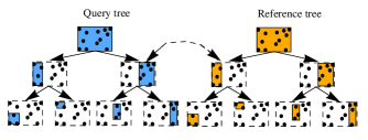
Figure 4: Top: A $kd$-tree partitions 2-dimensional points. Each node in the $kd$-tree records the bounding box for the subset of the dataset it contains (highlighted in color). In dual-tree recursion, a pair of nodes chosen from the query tree and the reference tree is considered at a time. Bottom: the lower and upper bound on pairwise distances between the points contained in each of the query/reference node pair.

Algorithm 3 $\mbox{{DualTree}}(Q,R)$: The dual-tree main routine.

  if CanSummarize$(Q,R,\epsilon)$ then

     Summarize$(Q,R)$

  else

     if $Q$ is a leaf node then

        if $R$ is a leaf node then

           $\mbox{{DualTreeBase}}(Q,R)$

        else

           $\mbox{{DualTree}}(Q,R^{L})$,          $\mbox{{DualTree}}(Q,R^{R})$

     else

        if $R$ is a leaf node then

           $\mbox{{DualTree}}(Q^{L},R)$,          $\mbox{{DualTree}}(Q^{R},R)$

        else

           $\mbox{{DualTree}}(Q^{L},R^{L})$,        $\mbox{{DualTree}}(Q^{L},R^{R})$

           $\mbox{{DualTree}}(Q^{R},R^{L})$,        $\mbox{{DualTree}}(Q^{R},R^{R})$

These distance bounds can be computed in $O(D)$ time using:

$$d^{l}(Q,R) =\frac{1}{2}\sqrt{\sum\limits_{k=1}^{D}\left(d^{l,u}_{j,i}[k]+\left|d^{l,u}_{j,i}[k]\right|+d^{l,u}_{i,j}[k]+\left|d^{l,u}_{i,j}[k]\right|\right)^{2}}$$ (6)

$$d^{u}(Q,R) =\sqrt{\sum\limits_{k=1}^{D}\left(\max\left\{d^{u,l}_{j,i}[k],d_{i,j}^{u,l}[k]\right\}\right)^{2}}$$ (7)

where $d^{l,u}_{j,i}[k]=R^{l}[k]-Q^{u}[k]$, $d^{l,u}_{i,j}[k]=Q^{l}[k]-R^{u}[k]$, $d^{u,l}_{j,i}[k]=R^{u}[k]-Q^{l}[k]$,
$d^{u,l}_{i,j}[k]=Q^{u}[k]-R^{l}[k]$. The CanSummarize function tests whether it is possible to summarize the sum contribution of the given reference node for each query point in the given query node. If possible, the Summarize function approximates the sum contribution of the given reference node; we then say the given pair of the query node and the reference node has been pruned. The idea is to prune unneeded portions of the dual-tree traversal, thereby minimizing the number of exhaustive leaf-leaf computations.

3 Dual-Tree Fast Gauss Transform

3.1 Mathematical Preliminaries

Univariate Taylor’s Theorem. The univariate Taylor’s theorem is crucial for the approximation mechanism in Fast Gauss transform and our new algorithm:

Theorem 3.1.

If $n\geq 0$ is an integer and $f$ is a function which is $n$ times continuously differentiable on the closed interval $[c,x]$ and $n+1$ times differentiable on $(c,x)$ then

$$f(x)=\sum\limits_{i=0}^{n}f^{(i)}(c)\frac{(x-c)^{i}}{i!}+R_{n}$$ (8)

where the Lagrange form of the remainder term is given by
$R_{n}=f^{(n+1)}(\xi)\frac{(x-c)^{n+1}}{(n+1)!}$ for some $\xi\in(c,x)$.

Multi-index Notation. Throughout this paper, we will be using the multi-index notation. A $D$-dimensional multi-index $\alpha$ is a $D$-tuple of non-negative integers. For any $D$-dimensional multi-indices $\alpha$, $\beta$ and any $x\in\mathbb{R}^{D}$,

• $|\alpha|=\alpha[1]+\alpha[2]+\cdots+\alpha[D]$

• $\alpha!=(\alpha[1])!(\alpha[2])!\cdots(\alpha[D])!$

• $x^{\alpha}=(x[1])^{\alpha[1]}(x[2])^{\alpha[2]}\cdots(x[D])^{\alpha[D]}$

• $D^{\alpha}=\partial_{1}^{\alpha[1]}\partial_{2}^{\alpha[2]}\cdots\partial_{D}^{\alpha[D]}$

• $\alpha+\beta=(\alpha[1]+\beta[1],\cdots,\alpha[D]+\beta[D])$

• $\alpha-\beta=(\alpha[1]-\beta[1],\cdots,\alpha[D]-\beta[D])$ for $\alpha\geq\beta$.

where $\partial_{i}$ is a $i$-th directional partial derivative. Define $\alpha>\beta$ if $\alpha[d]>\beta[d]$, and $\alpha\geq p$ for $p\in\mathbb{Z^{+}}\cup\{0\}$ if $\alpha[d]\geq p$ for $1\leq d\leq D$ (and similarly for $\alpha\leq p$).

Properties of the Gaussian Kernel. Based on the univariate Taylor’s Theorem stated above, [11] develops the series expansion mechanism for the Gaussian kernel sum. Our development begins with one-dimensional setting and generalizes to multi-dimensional setting. We first define the Hermite polynomials by the Rodrigues’ formula:

$$\begin{split}H_{n}(t)=(-1)^{n}e^{t^{2}}D^{n}e^{-t^{2}},t\in\mathbb{R}^{1}\end{split}$$ (9)

The first few polynomials include: $H_{0}(t)=1$, $H_{1}(t)=2t$, $H_{2}(t)=4t^{2}-2$. The generating function for Hermite polynomials is defined by:

$$\begin{split}e^{2ts-s^{2}}=\sum\limits_{n=0}^{\infty}\frac{s^{n}}{n!}H_{n}(t)\end{split}$$ (10)

Let us define the Hermite functions $h_{n}(t)$ by

$$\begin{split}h_{n}(t)=e^{-t^{2}}H_{n}(t)\end{split}$$ (11)

Multiplying both sides by $e^{-t^{2}}$ yields:

$$\begin{split}e^{-(t-s)^{2}}=\sum\limits_{n=0}^{\infty}\frac{s^{n}}{n!}h_{n}(t)\end{split}$$ (12)

We would like to use a “scaled and shifted” version of this derivation for taking the bandwidth $h$ into account.

$$e^{\frac{-(t-s)^{2}}{2h^{2}}} =e^{\frac{-((t-s_{0})-(s-s_{0}))^{2}}{2h^{2}}}=\sum\limits_{n=0}^{\infty}\frac{1}{n!}\left(\frac{s-s_{0}}{\sqrt{2h^{2}}}\right)^{n}h_{n}\left(\frac{t-s_{0}}{\sqrt{2h^{2}}}\right)$$ (13)

Note that our $D$-dimensional multivariate Gaussian kernel can be expressed as a product of $D$ one-dimensional Gaussian kernel. Similarly, the multidimensional Hermite functions can be written as a product of one-dimensional Hermite functions using the following identity for any $t\in\mathbb{R^{D}}$.

$$\begin{split}H_{\alpha}(t)&=H_{\alpha[1]}(t[1])\cdots H_{\alpha[D]}(t[D])\\ h_{\alpha}(t)&=e^{-||t||^{2}}H_{\alpha}(t)=h_{\alpha[1]}(t[1])\cdots h_{\alpha[D]}(t[D])\\ \end{split}$$ (14)

where $||t||^{2}=(t[1])^{2}+\cdots+(t[D])^{2}$.

$$\begin{split}e^{\frac{-||t-s||^{2}}{2h^{2}}}&=e^{\frac{-(t[1]-s[1])^{2}-(t[2]-s[2])^{2}-\cdots-(t[D]-s[D])^{2}}{2h^{2}}}\\ &=e^{\frac{-(t[1]-s[1])^{2}}{2h^{2}}}e^{\frac{-(t[2]-s[2])^{2}}{2h^{2}}}\cdots e^{\frac{-(t[D]-s[D])^{2}}{2h^{2}}}\\ \end{split}$$ (15)

We can also express the multivariate Gaussian about another point $s_{0}\in\mathbb{R}^{D}$ as:

$$\begin{split}e^{\frac{-||t-s||^{2}}{2h^{2}}}&=\prod\limits_{d=1}^{D}\left(\sum\limits_{n_{d}=0}^{\infty}\frac{1}{n_{d}!}\left(\frac{s[d]-s_{0}[d]}{\sqrt{2h^{2}}}\right)^{n_{d}}h_{n_{d}}\left(\frac{t[d]-s_{0}[d]}{\sqrt{2h^{2}}}\right)\right)\\ &=\sum\limits_{\alpha\geq 0}\frac{1}{\alpha!}\left(\frac{s-s_{0}}{\sqrt{2h^{2}}}\right)^{\alpha}h_{\alpha}\left(\frac{t-s_{0}}{\sqrt{2h^{2}}}\right)\\ \end{split}$$ (16)

The representation which is dual to Equation (16) is given by:

$$\begin{split}e^{\frac{-||t-s||^{2}}{2h^{2}}}&=\prod\limits_{d=1}^{D}\left(\sum\limits_{n_{d}=0}^{\infty}\frac{(-1)^{n_{d}}}{n_{d}!}h_{n_{d}}\left(\frac{t_{0}[d]-s(d)}{\sqrt{2h^{2}}}\right)\left(\frac{t[d]-t_{0}}{\sqrt{2h^{2}}}\right)^{\beta}\right)\\ &=\sum\limits_{\beta\geq 0}\frac{(-1)^{\beta}}{\beta!}h_{\beta}\left(\frac{t_{0}-s}{\sqrt{2h^{2}}}\right)\left(\frac{t-t_{0}}{\sqrt{2h^{2}}}\right)^{\beta}\end{split}$$ (17)

The final property is the recurrence relation of the one-dimensional Hermite function:

$$\begin{split}h_{n+1}(t)=2t\cdot h_{n}(t)-2n\cdot h_{n-1}(t),t\in\mathbb{R}^{1}\end{split}$$ (18)

and the Taylor expansion of the Hermite function $h_{\alpha}(t)$ about $t_{0}\in\mathbb{R^{D}}$.

$$\begin{split}h_{\alpha}(t)=\sum\limits_{\beta\geq 0}\frac{(t-t_{0})^{\beta}}{\beta!}(-1)^{|\beta|}h_{\alpha+\beta}(t_{0})\\ \end{split}$$ (19)

3.2 Notations in Algorithm Descriptions

Here we summarize notations used throughout the descriptions and the pseudocodes for our algorithms. The followings are notations that are relevant to a query point $q_{i}\in\mathcal{Q}$ or a query node $Q$ in the query tree.

• $\mathcal{R_{E}}(\cdot)$: The set of reference points $r_{j_{n}}\in\mathcal{R}$ whose pairwise interaction is computed exhaustively for a query point $q_{i}\in\mathcal{Q}$ or a query node $Q$.

• $\mathcal{R_{T}}(\cdot)$: The set of reference points $r_{j_{n}}\in\mathcal{R}$ whose contribution is pruned via centroid-based approximation for a given query point $q_{i}\in\mathcal{Q}$.

The followings are notations relevant to a query point $q_{i}\in\mathcal{Q}$.

• $G(q_{i},R)$: The true initially unknown kernel sum for a query point $q_{i}$ contributed by the reference set $R\subseteq\mathcal{R}$, i.e. $\sum\limits_{r_{j_{n}}\in R}K_{h}(||q_{i}-r_{j_{n}}||)$.

• $G^{l}(q_{i},\mathcal{R})$: A lower bound on $G(q_{i},\mathcal{R})$.

• $G^{u}(q_{i},\mathcal{R})$: An upper bound on $G(q_{i},\mathcal{R})$.

• $\widetilde{G}(q_{i},R)$: An approximation to $G(q_{i},R)$ for $R\subseteq\mathcal{R}$. This obeys the additive property for a family of pairwise disjoint sets $\{R_{i}\}_{i=1}^{m}$: $\widetilde{G}\left(q_{i},\bigcup\limits_{i=1}^{m}R_{i}\right)=\sum\limits_{i=1}^{m}\widetilde{G}(q_{i},R_{i})$.

• $\widetilde{G}\left(q_{i},\{(R_{j},A_{j})\}_{j=1}^{m}\right)$: A refined notation of $\widetilde{G}\left(q_{i},\bigcup\limits_{j=1}^{m}R_{j}\right)$ to specify the type of approximation used for each reference node $R_{j}$.

Here we define some notations for representing postponed bound changes to $G^{l}(q_{i_{m}},\mathcal{R})$ and $G^{u}(q_{i_{m}},\mathcal{R})$ for all $q_{i_{m}}\in Q$.

• $Q.\Delta^{l}$: Postponed lower bound changes on $G^{l}(q_{i_{m}},\mathcal{R})$ for a query node $Q$ in the query tree and $q_{i}\in Q$.

• $Q.L$: Postponed changes to $\widetilde{G}(q_{i_{m}},\mathcal{R_{T}}(q_{i_{m}}))$ for $q_{i_{m}}\in Q$.

• $Q.\Delta^{u}$: Postponed upper bound changes on $G^{l}(q_{i_{m}},\mathcal{R})$ for a query node $Q$ in the query tree and $q_{i}\in Q$.

These postponed changes to the upper and lower bounds must be incorporated into each individual query $q_{i_{m}}$ belonging to the sub-tree under $Q$.

Our series-expansion based algorithm uses four different approximation methods, i.e. $A\in\{E,T(c,p),F(c,p),D(c,p)\}$. $E$ again denotes the exhaustive computation of $\sum\limits_{r_{j_{n}}\in R}K_{h}(||q_{i}-r_{j_{n}}||)$. $T(c,p)$ denotes the translation of the order $p-1$ far-field moments of $R$ to the local moments in the query node $Q$ that owns $q_{i}$ about a representative centroid $c$ inside $Q$. $F(c,p)$ denotes the evaluation of the order $p-1$ far-field expansion formed by the moments of $R$ expanded about a representative point $c$ inside $R$. $D(c,p)$ denotes the $p-1$th order direct accumulation of the local moments due to $R$ about a representative centroid $c$ inside $Q$ that owns $q_{i}$. We discuss these approximation methods in Section 3.3.

3.3 Series Expansion for the Gaussian Kernel Sums

We would like to point out to our readers that we present the series expansion in a way that sheds light to a working implementation. [11] chose a theorem-proof format for explaining the essential operations. We present the series expansion methods from the more informed computer science perspective of divide-and-conquer and data structures, where the discrete aspects of the methods are concerned.

One can derive the series expansion for the Gaussian kernel sums (defined in Equation (5)) using Equation (16) and Equation (17). The basic idea is to express the kernel sum contribution of a reference node as a Taylor series of infinite terms and truncate it after some number of terms, given that the truncation error meets the desired absolute error tolerance.

The followings are two main types of Taylor series representations for infinitely differentiable kernel functions $K_{h}\left(\cdot\right)$’s. The key difference between two representations is the location of the expansion center which is either in a reference region or a query region. The center of the expansion for both types of expansions is conveniently chosen to be the geometric center of the region. For the node region $N$ bounded by $[N.b[1].l,N.b[1].u]\times\cdots\times[N.b[D].l,N.b[D].u]$, the center is $N.c=\left[\frac{N.b[1].l+N.b[1].u}{2},\cdots,\frac{N.b[D].l+N.b[D].u}{2}\right]^{T}$.

1. Far-field expansion: A far-field expansion (derived from Equation (16)) expresses the kernel sum contribution from the reference points in the reference node $R$ for an arbitrary query point. It is expanded about $R.c$, a representative point of $R$. Equation (16) is an infinite series, and thus we impose a truncation order $p$ in each dimension. Substituting $q_{i}$ for $t$, $r_{j}$ for $s$ and $R.c$ for $s_{0}$ into Equation (16) yields:

   $$G(q_{i},R)=\sum\limits_{r_{j_{n}}\in R}e^{\frac{-||q_{i}-r_{j_{n}}||^{2}}{2h^{2}}}$$

   $$= \sum\limits_{r_{j_{n}}\in R}\prod\limits_{d=1}^{D}\left(\sum\limits_{\alpha[d]=0}^{\infty}\frac{1}{\alpha[d]!}\left(\frac{r_{j_{n}}[d]-R.c[d]}{\sqrt{2h^{2}}}\right)^{\alpha[d]}h_{\alpha[d]}\left(\frac{q_{i}[d]-R.c[d]}{\sqrt{2h^{2}}}\right)\right)$$

   $$= \sum\limits_{r_{j_{n}}\in R}\prod\limits_{d=1}^{D}\Bigg{(}\sum\limits_{\alpha[d]<p}\frac{1}{\alpha[d]!}\left(\frac{r_{j_{n}}[d]-R.c[d]}{\sqrt{2h^{2}}}\right)^{\alpha[d]}h_{\alpha[d]}\left(\frac{q_{i}[d]-R.c[d)]}{\sqrt{2h^{2}}}\right)+$$

   $$\ \ \ \ \ \ \ \ \ \ \ \ \ \sum\limits_{\alpha[d]\geq p}\frac{1}{\alpha[d]!}\left(\frac{r_{j_{n}}[d]-R.c[d]}{\sqrt{2h^{2}}}\right)^{\alpha[d]}h_{\alpha[d]}\left(\frac{q_{i}[d]-R.c[d]}{\sqrt{2h^{2}}}\right)\Bigg{)}$$

   Truncating after $p$ terms along each dimension yields:

   $$G(q_{i},R)\approx\widetilde{G}(q_{i},\{(R,F(R.c,p))\})$$

   $$= \sum\limits_{r_{j_{n}}\in R}\prod\limits_{d=1}^{D}\left(\sum\limits_{\alpha[d]<p}\frac{1}{\alpha[d]!}\left(\frac{r_{j_{n}}[d]-R.c[d]}{\sqrt{2h^{2}}}\right)^{\alpha[d]}h_{\alpha[d]}\left(\frac{q_{i}[d]-R.c[d]}{\sqrt{2h^{2}}}\right)\right)$$

   $$= \sum\limits_{r_{j_{n}}\in R}\sum\limits_{\alpha<p}\frac{1}{\alpha!}\left(\frac{r_{j_{n}}-R.c}{\sqrt{2h^{2}}}\right)^{\alpha}h_{\alpha}\left(\frac{q_{i}-R.c}{\sqrt{2h^{2}}}\right)$$

   $$= \sum\limits_{\alpha<p}\left[\sum\limits_{r_{j_{n}}\in R}\frac{1}{\alpha!}\left(\frac{r_{j_{n}}-R.c}{\sqrt{2h^{2}}}\right)^{\alpha}\right]h_{\alpha}\left(\frac{q_{i}-R.c}{\sqrt{2h^{2}}}\right)$$

   $$= \sum\limits_{\alpha<p}M_{\alpha}(R,R.c)h_{\alpha}\left(\frac{q_{i}-R.c}{\sqrt{2h^{2}}}\right)$$

   where we denote

   $$M_{\alpha}(R,c)=\sum\limits_{r_{j_{n}}\in R}\frac{1}{\alpha!}\left(\frac{r_{j_{n}}-c}{\sqrt{2h^{2}}}\right)^{\alpha}$$ (20)

   which is a function of a reference node $R$ and an expansion center $c$. We denote $\widetilde{G}(q_{i},\{R,F(c,p)\})$ as the far-field expansion of order $p-1$ for the kernel sum contribution of $R$ expanded about $c$. Ideally, we would like to choose the smallest $p$ such that the truncation after the chosen order $p$ incurs tolerable error; this will be discussed in Section 3.5.

   

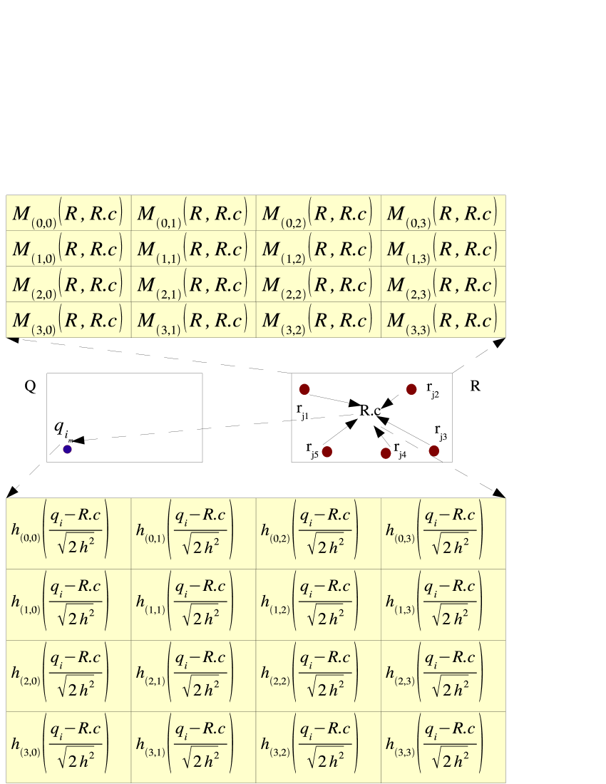
   Figure 5: Given the query node $Q$ containing the query points $\{q_{i_{m}}\}_{m=1}^{|Q|}$ and the reference node $R$ containing the reference points $\{r_{j_{n}}\}_{n=1}^{|R|}$, evaluating the far-field expansion generated by the reference points at the given query point $q_{i_{m}}$ up to four terms in each dimension, $G(q_{i_{m}},R)\approx\widetilde{G}(q_{i_{m}},\{(R,F(R.c,4))\})=\sum\limits_{\alpha<4}\left[\sum\limits_{r_{j_{n}}\in R}\frac{1}{\alpha!}\left(\frac{r_{j_{n}}-R.c}{\sqrt{2h^{2}}}\right)^{\alpha}\right]h_{\alpha}\left(\frac{q_{i_{m}}-R.c}{\sqrt{2h^{2}}}\right)$, involves computing the sum of the element-wise product between the two-dimensional array of far-field coefficients with the query-dependent two-dimensional array.

   Note that the far-field expansion for the Gaussian kernel separates the interaction between a reference point and a query point (namely $e^{-||q_{i}-r_{j_{n}}||^{2}/(2h^{2})}$) into a summation of two product terms. For each multi-index $\alpha$, $M_{\alpha}(R,R.c)$, which depends only on the intrinsic information for the reference node (the reference points $r_{j_{n}}\in R$ and the reference centroid $R.c$ which is constant with respect to $R$), is called the far-field moments/coefficients of the reference region $R$. Because $M_{\alpha}(R,R.c)$ part of the far-field expansion of the Gaussian kernel sums is the same regardless of the query point $q_{i}$ used for evaluation, they can be computed only once and stored within $R$ for efficiently approximating the contribution of $R$ for different query points (see Figure 5). Precomputing the far-field moments for a reference node $R$ up to $p^{D}$ terms (i.e. computing $\sum\limits_{r_{j_{n}}\in R}\frac{1}{\alpha!}\left(\frac{r_{j_{n}}-R.c}{\sqrt{2h^{2}}}\right)^{\alpha}$ for each $\alpha<p$) requires $O(|R|p^{D})$ operations.

   The far-field expansion of order $p-1$ for the Gaussian kernel sums is valid for any query locations $q_{i}$ given that the reference node meets the certain size constraint (see Section 3.5). However, for a fixed order $p$, evaluating on query points that are far away from the reference centroid in general incur smaller amount of error.

   

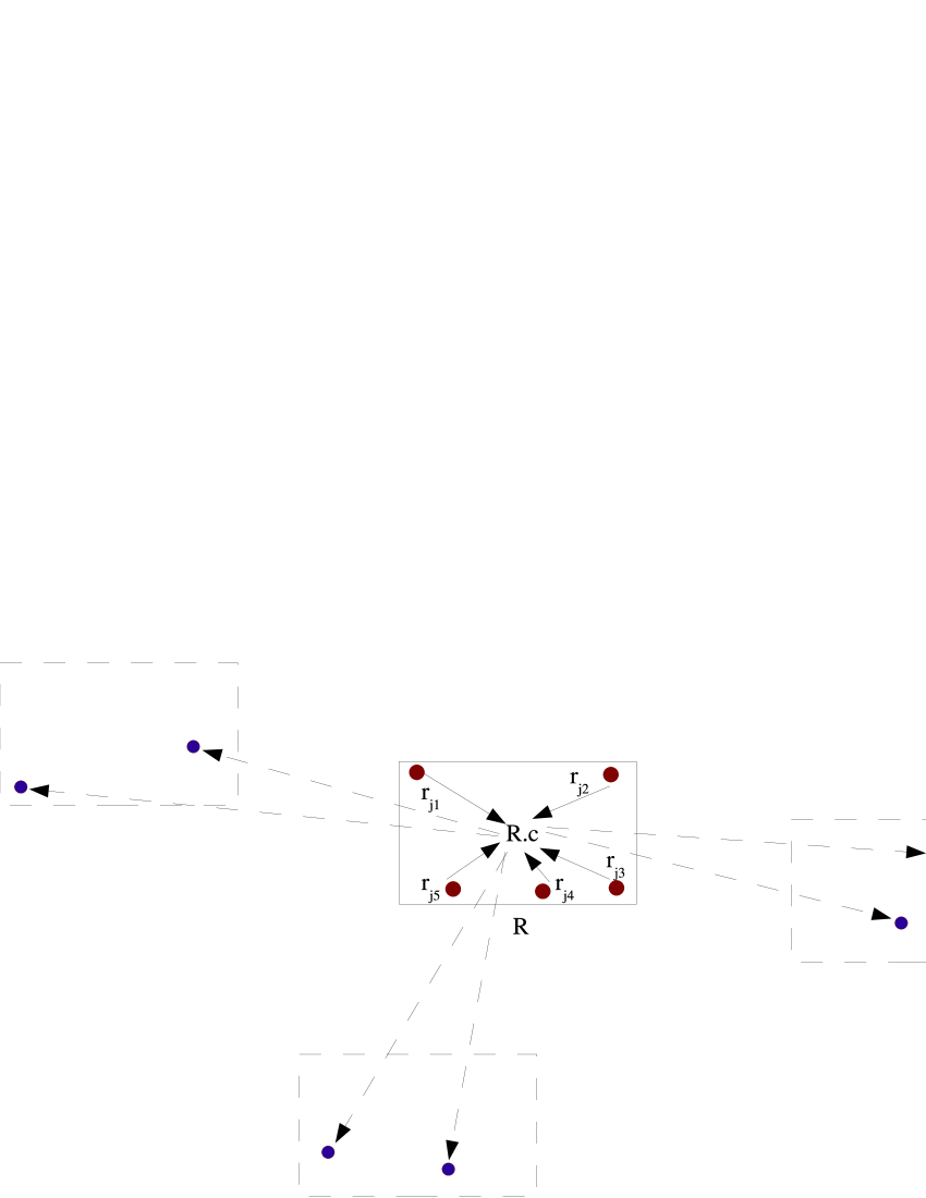
   Figure 6: The Gaussian kernel sum series expansion represented by the far-field coefficients in $R$, $\sum\limits_{\alpha<p}M_{\alpha}(R,R.c)h_{\alpha}\left(\frac{r_{j_{n}}-R.c}{\sqrt{2h^{2}}}\right)$, is valid regardless of the location of the given query point, given the size constraint on the reference node (see Section 3.5). However, each query point location will incur different amount of error.

2. Local expansion: A local expansion (derived from Equation (17)) is a Taylor expansion of the kernel sums about a representative point $Q.c$ in a query region $Q$. After substituting $q_{i}$ for $t$, $Q.c$ for $t_{0}$ and $r_{j_{n}}$ for $s$, the kernel sum contribution of all reference points in a reference region $R$ to a query point $q_{i}\in Q$ is given by:

   $$G(q_{i},R)=\sum\limits_{r_{j_{n}}\in R}e^{\frac{-||q_{i}-r_{j_{n}}||^{2}}{2h^{2}}}$$

   $$= \sum\limits_{r_{j_{n}}\in R}\prod\limits_{d=1}^{D}\left(\sum\limits_{n_{d}=0}^{\infty}\frac{(-1)^{n_{d}}}{n_{d}!}h_{n_{d}}\left(\frac{Q.c[d]-r_{j_{n}}[d]}{\sqrt{2h^{2}}}\right)\left(\frac{q_{i}[d]-Q.c[d]}{\sqrt{2h^{2}}}\right)^{\beta}\right)$$

   $$= \sum\limits_{r_{j_{n}}\in R}\prod\limits_{d=1}^{D}\Biggl{(}\sum\limits_{n_{d}<p}\frac{(-1)^{n_{d}}}{n_{d}!}h_{n_{d}}\left(\frac{Q.c[d]-r_{j_{n}}[d]}{\sqrt{2h^{2}}}\right)\left(\frac{q_{i}[d]-Q.c[d]}{\sqrt{2h^{2}}}\right)^{\beta}+$$

   $$\ \ \ \ \ \ \ \ \ \ \ \ \ \sum\limits_{n_{d}\geq p}\frac{(-1)^{n_{d}}}{n_{d}!}h_{n_{d}}\left(\frac{Q.c[d]-r_{j_{n}}[d]}{\sqrt{2h^{2}}}\right)\left(\frac{q_{i}[d]-Q.c[d]}{\sqrt{2h^{2}}}\right)^{\beta}\Biggr{)}$$

   Again, truncating after $p$ terms along each dimension yields:

   $$\widetilde{G}(q_{i},\{(R,D(Q.c,p))\})$$

   $$= \sum\limits_{r_{j_{n}}\in R}\prod\limits_{d=1}^{D}\left(\sum\limits_{n_{d}<p}\frac{(-1)^{n_{d}}}{n_{d}!}h_{n_{d}}\left(\frac{Q.c[d]-r_{j_{n}}[d]}{\sqrt{2h^{2}}}\right)\left(\frac{q_{i}[d]-Q.c[d]}{\sqrt{2h^{2}}}\right)^{\beta}\right)$$

   $$= \sum\limits_{r_{j_{n}}\in R}\sum\limits_{\beta<p}\frac{(-1)^{\beta}}{\beta!}h_{\beta}\left(\frac{Q.c-r_{j_{n}}}{\sqrt{2h^{2}}}\right)\left(\frac{q_{i}-Q.c}{\sqrt{2h^{2}}}\right)^{\beta}$$

   $$= \sum\limits_{\beta<p}\left[\sum\limits_{r_{j_{n}}\in R}\frac{(-1)^{\beta}}{\beta!}h_{\beta}\left(\frac{Q.c-r_{j_{n}}}{\sqrt{2h^{2}}}\right)\right]\left(\frac{q_{i}-Q.c}{\sqrt{2h^{2}}}\right)^{\beta}$$

   $$= \sum\limits_{\beta<p}L_{\beta}(\{(R,D(Q.c,p))\})\left(\frac{q_{i}-Q.c}{\sqrt{2h^{2}}}\right)^{\beta}$$

   where we denote:

   $$L_{\beta}(\{(R,D(c,p))\})=\begin{cases}\sum\limits_{r_{j_{n}}\in R}\frac{(-1)^{\beta}}{\beta!}h_{\beta}\left(\frac{c-r_{j_{n}}}{\sqrt{2h^{2}}}\right)&,\mbox{$\beta<p$}\\ 0&,\mbox{otherwise}\end{cases}$$ (21)

   $\{L_{\beta}(\{(R,D(Q.c,p))\})\}_{\beta}$ are the direct local moments of $R$ for $Q$. The error bound criterion will be discussed in Section 3.5. Note that:

   $$\widetilde{G}\left(q_{i},\bigcup\limits_{a}\left\{(R_{a},D(p_{a}))\right\}\right)=\sum\limits_{a}\widetilde{G}(q_{i},\{(R_{a},D(p_{a}))\})$$

   $$= \sum\limits_{a}\sum\limits_{\beta<p_{a}}\left[\sum\limits_{r_{j_{n}}\in R_{a}}\frac{(-1)^{\beta}}{\beta!}h_{\beta}\left(\frac{Q.c-r_{j_{n}}}{\sqrt{2h^{2}}}\right)\right]\left(\frac{q_{i}-Q.c}{\sqrt{2h^{2}}}\right)^{\beta}$$

   $$= \sum\limits_{\beta<\max\limits_{a}p_{a}}\left[\sum\limits_{a}L_{\beta}(\{(R_{a},D(Q.c,p_{a}))\})\right]\left(\frac{q_{i}-Q.c}{\sqrt{2h^{2}}}\right)^{\beta}$$

   $$= \sum\limits_{\beta<\max\limits_{a}p_{a}}L_{\beta}\left(\bigcup\limits_{a}\left\{(R_{a},D(Q.c,p_{a}))\right\}\right)\left(\frac{q_{i}-Q.c}{\sqrt{2h^{2}}}\right)^{\beta}$$

   In other words, the local moments for a fixed query node $Q$ are additive (see Figure 8) across a set of disjoint portions of the reference dataset $\mathcal{R}$ since its basis functions $\left\{\left(\frac{q_{i}-Q.c}{\sqrt{2h^{2}}}\right)^{\beta}\right\}_{\beta}$ remain the same for all reference points regardless of their locations. For a given reference node $R$, accumulating the local moments of $R$ up to $p^{D}$ terms (that is, evaluating for each $\beta<p$) requires $O(|R|p^{D})$ operations. These local coefficients are accumulated and stored within the given query node. The local expansion represented by the local coefficients is valid for all query points within the query node under certain constraints.

   

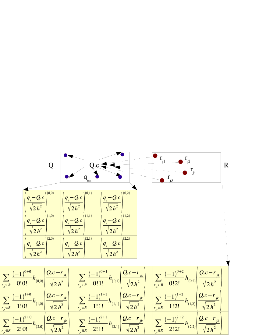
   Figure 7: Given the query node $Q$ containing the query points $\{q_{i_{m}}\}_{m=1}^{|Q|}$ and the reference node $R$ containing the reference points $\{r_{j_{n}}\}_{n=1}^{|R|}$, evaluating the local expansion generated by the reference points at the given query point $q_{i_{m}}$ up to third terms in each dimension, $G(q_{i_{m}},R)\approx\widetilde{G}(q_{i_{m}},\{(R,D(Q.c,3))\})=\sum\limits_{\beta<3}\left[\sum\limits_{r_{j_{n}}\in R}\frac{(-1)^{\beta}}{\beta!}h_{\beta}\left(\frac{Q.c-r_{j_{n}}}{\sqrt{2h^{2}}}\right)\right]\left(\frac{q_{i_{m}}-Q.c}{\sqrt{2h^{2}}}\right)^{\beta}$, involves taking the dot-product between the two-dimensional array of local coefficients with the query-dependent two-dimensional array.

   

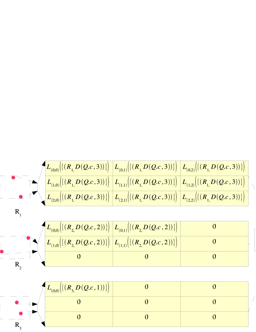
   Figure 8: Accumulating direct local moments from three reference nodes with the nodes $R_{1}$, $R_{2}$, and $R_{3}$ contributing nine terms, four terms, and one term respectively to form the local moments containing the contribution from $R_{1}$, $R_{2}$, and $R_{3}$: $L(\{(R_{1},D(Q.c,3)),(R_{2},D(Q.c,2)),(R_{3},D(Q.c,1))\})$. Zeros denote the positions that are not explicitly computed using Equation (21). $L(\{(R_{1},D(Q.c,3)),(R_{2},D(Q.c,2)),(R_{3},D(Q.c,1))\})=L(\{(R_{1},D(Q.c,3))\})+L(\{(R_{2},D(Q.c,2))\})+L(\{(R_{3},D(Q.c,1))\})$ is added to the total local moments for $Q$.

   

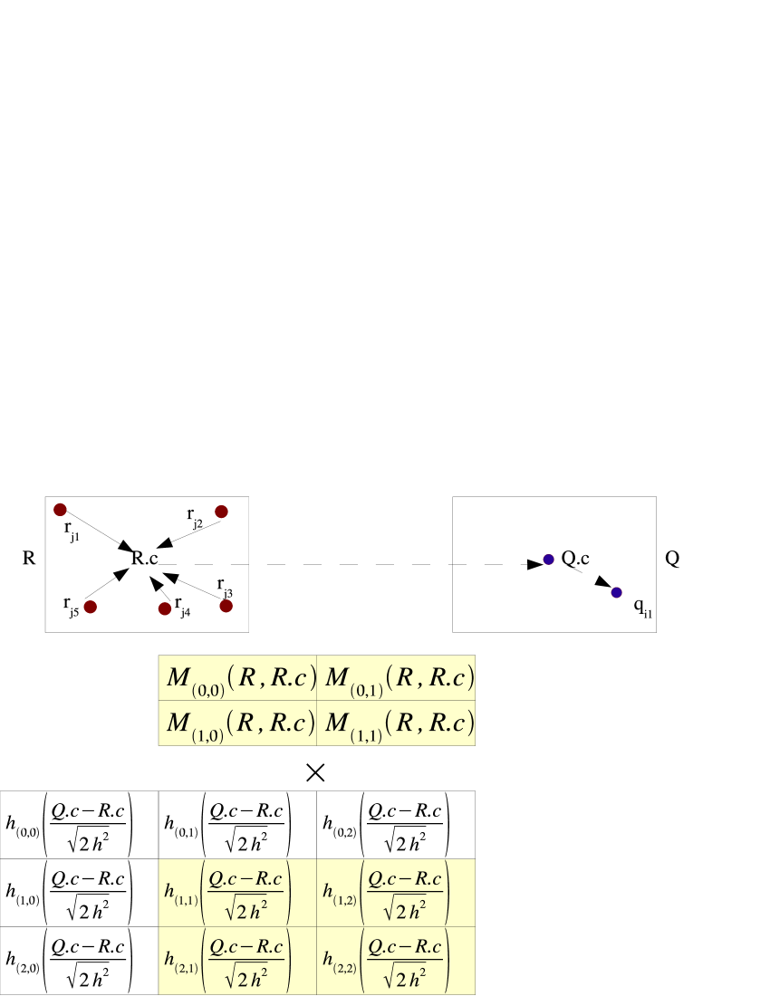
   Figure 9: Two-dimensional far-field coefficients truncated after the first two terms in each dimension can be converted into a set of local moments using Equation (22). Computing $L_{\beta}(\{(R,T(Q.c,2))\})$ involves summing up the element-wise product between the matrix (or tensor in higher dimensions) consisting of the far-field moments and the two-by-two window over the Hermite functions whose upper left multi-index is $\beta$. This figure shows how to compute $L_{(1,1)}(\{(R,T(Q.c,2))\})$.

3.4 Gaussian Sum Approximation Using Series Expansion

Now again assume we are given a query node $Q$ and a reference node $R$. Here we describe three main methods that use the two expansion types for approximating Gaussian summation, $\widetilde{G}(q,R)$, for each $q\in Q$.

1. Evaluating a far-field expansion of $R$: Given the pre-computed far-field moments $M_{\alpha}(R)$ up to $p^{D}$ terms, one could evaluate the far-field expansion for a given query point $q$ (that is, approximate $\widetilde{G}(q,R)$) by forming a dot-product between the query-dependent vector and the far-field moments, as shown in Figure 5 and Figure 6. Approximating $\widetilde{G}(q,R)$ for all $q\in Q$ requires $O(|Q|p^{D})$ operations since evaluating the far-field expansion each time requires $O(p^{D})$ operations.

2. Computing and evaluating a local expansion inside $Q$ due to the contribution of $R$: one could iterate over each reference point $r_{j_{n}}\in R$ and compute the local moments $L_{\beta}(\{(R,D(Q.c,p))\})$ due to $R$ up to $p^{D}$ terms, as shown in Figure 7 and Figure 8. The local accumulation of the contribution of the reference node $R$ requires $O(|R|p^{D})$ operations, and evaluating the local expansion for each $q_{i_{m}}\in Q$ requires a total of $O(|Q|p^{D})$ operations.

3. Converting far-field moments of $R$ to a local expansion of $Q$: Suppose $R$ has pre-computed far-field moments up to $p^{D}$ terms. From the far-field moments, we can approximate the local moments of $R$ but with some amount of error. This can be seen as a generalization of centroid-based approximation.  [11] describes this method as one of the translation operators, called far-field to local translation operator, stated below:

   Lemma 3.2.

   Far-field to local (F2L) translation operator for Gaussian kernel (as presented in Lemma 2.2 in [11]): Given a reference node $R$, a query node $Q$, and the truncated far-field expansion centered at a centroid $R.c$ of $R$ up to $p^{D}$ terms:
   $\widetilde{G}(q_{i_{m}},\{(R,F(R.c,p))\})=\sum\limits_{\alpha<p}M_{\alpha}(R,R.c)h_{\alpha}\left(\frac{q_{i_{m}}-R.c}{\sqrt{2h^{2}}}\right)$,
   the Taylor expansion of the far-field expansion at the centroid $Q.c$ in $Q$ is given by $\widetilde{G}(q_{i_{m}},\{(R,F(R.c,p))\})=\sum\limits_{\beta\geq 0}L_{\beta}(\{(R,T(Q.c,p))\})\left(\frac{q_{i_{m}}-Q.c}{\sqrt{2h^{2}}}\right)^{\beta}$ where for $q_{i_{m}}\in Q$,

   $$L_{\beta}(\{(R,T(Q.c,p))\})=\frac{(-1)^{|\beta|}}{\beta!}\sum\limits_{\alpha<p}M_{\alpha}(R,R.c)h_{\alpha+\beta}\left(\frac{Q.c-R.c}{\sqrt{2h^{2}}}\right)$$ (22)

   Proof.

   The proof consists of replacing the Hermite function portion of the expansion with its Taylor series:

   $$\widetilde{G}(q_{i_{m}},\{(R,F(R.c,p))\})=\sum\limits_{\alpha<p}M_{\alpha}(R,R.c)h_{\alpha}\left(\frac{q_{i_{m}}-R.c}{\sqrt{2h^{2}}}\right)$$

   $$= \sum\limits_{\alpha<p}M_{\alpha}(R,R.c)\sum\limits_{\beta\geq 0}\frac{(-1)^{|\beta|}}{\beta!}h_{\alpha+\beta}\left(\frac{Q.c-R.c}{\sqrt{2h^{2}}}\right)\left(\frac{q_{i_{m}}-Q.c}{\sqrt{2h^{2}}}\right)^{\beta}$$

   $$= \sum\limits_{\beta\geq 0}\left[\frac{(-1)^{|\beta|}}{\beta!}\sum\limits_{\alpha<p}M_{\alpha}(R,R.c)h_{\alpha+\beta}\left(\frac{Q.c-R.c}{\sqrt{2h^{2}}}\right)\right]\left(\frac{q_{i_{m}}-Q.c}{\sqrt{2h^{2}}}\right)^{\beta}$$

   ∎

   However, note $\widetilde{G}(q_{i_{m}},\{(R,F(R.c,p))\})$ has an infinite number of terms, and must be truncated after $p^{D}$ terms. In other words, the local moments accumulated for $Q$ are the coefficients for $\widetilde{G}(q_{i_{m}},\{(R,T(Q.c,p))\})=\sum\limits_{\beta<p}L_{\beta}(\{(R,T(Q.c,p))\})\left(\frac{q_{i_{m}}-Q.c}{\sqrt{2h^{2}}}\right)^{\beta}$, as shown in Figure 9. To compute $\{L_{\beta}(\{(R,T(Q.c,p))\})\}_{\beta<p}$, we need to iterate over all of $p^{D}$ far-field moments $\{M_{\alpha}(R,R.c)\}_{\alpha<p}$ for each $L_{\beta}(\{(R,T(Q.c,p))\})$. This operation runs in $O(Dp^{2D})$ operations.

In general, these approximations are valid only under certain conditions which depend on how the error bounds associated with these approximation methods are derived. Moreover, we have not discussed how to choose the method of approximation given a query and reference node pair, and how to determine the order of approximation, i.e. the number of terms required to achieve a given level of error. We discuss the details in Section 3.5.

3.5 Truncation Error Bounds

Because the far-field and the local expansions are truncated after taking $p^{D}$ terms, we incur an error in approximation. The original error bounds for the Gaussian kernel in [11] were wrong and corrections were shown in [3]. Here we present the error bounds for (1) evaluating a truncated far-field expansion of a reference node for any query point $q\in\mathbb{R}^{D}$ (2) evaluating a truncated local expansion of $Q$ due to the contribution of a reference node $R$ for any query point $q_{i_{m}}\in Q$ (3) evaluating a truncated local expansion formed from converting a truncated far-field expansion of a reference node $R$ for any query point $q_{i_{m}}\in Q$. Note that these error bounds place restrictions on the size of the nodes in consideration: reference node, query node, or both. First we start with the truncation error bound for evaluating the far-field expansion formed for a given reference node.

Lemma 3.3.

Error bound for evaluating a truncated far-field expansion (as presented in [3]): Suppose we are given a far-field expansion of a reference node $R$ about its centroid $R.c$:
$\widetilde{G}(q,\{(R,F(R.c,p))\})=\sum\limits_{\alpha<p}M_{\alpha}(R,R.c)h_{\alpha}\left(\frac{q-R.c}{\sqrt{2h^{2}}}\right)$ where
$M_{\alpha}(R,R.c)=\sum\limits_{r_{j_{n}}\in R}\frac{1}{\alpha!}\left(\frac{r_{j_{n}}-R.c}{\sqrt{2h^{2}}}\right)^{\alpha}$. If $\forall r_{j_{n}}\in R$ satisfies $||r_{j_{n}}-R.c||_{\infty}<rh$ for $r<1$, then for any $q\in\mathbb{R}^{D}$,

$$\left|\widetilde{G}(q,\{(R,F(R.c,p))\})-G(q,R)\right|\leq\frac{|R|}{(1-r)^{D}}\sum\limits_{k=0}^{D-1}\binom{D}{k}(1-r^{p})^{k}\left(\frac{r^{p}}{\sqrt{p!}}\right)^{D-k}$$ (23)

Proof.

We expand the far-field expansion as a product of one-dimensional Hermite functions, and utilize a bound on one-dimensional Hermite functions due to [17]: $\frac{1}{n!}|h_{n}(x)|\leq\frac{2^{\frac{n}{2}}}{\sqrt{n!}}e^{\frac{-x^{2}}{2}},n\geq 0,x\in\mathbb{R}^{1}$.

$$u_{p_{d}}(q[d],r_{j_{n}}[d],R.c[d]) =\sum\limits_{n_{i}=0}^{p-1}\frac{1}{n_{i}!}\left(\frac{r_{j_{n}}[d]-R.c[d]}{\sqrt{2h^{2}}}\right)^{n_{i}}h_{n_{i}}\left(\frac{q[d]-R.c[d]}{\sqrt{2h^{2}}}\right)$$

$$v_{p_{d}}(q[d],r_{j_{n}}[d],R.c[d]) =\sum\limits_{n_{i}=p}^{\infty}\frac{1}{n_{i}!}\left(\frac{r_{j_{n}}[d]-R.c[d]}{\sqrt{2h^{2}}}\right)^{n_{i}}h_{n_{i}}\left(\frac{q[d]-R.c[d]}{\sqrt{2h^{2}}}\right)$$

$$e^{\frac{-||q-r_{j_{n}}||^{2}}{{2h^{2}}}} =\prod\limits_{d=1}^{D}\left(u_{p_{d}}(q[d],r_{j_{n}}[d],R.c[d])+v_{p_{d}}(q[d],r_{j_{n}}[d],R.c[d])\right)$$

We obtain for $1\leq d\leq D$:

$$u_{p_{d}}(q[d],r_{j_{n}}[d],R.c[d])\leq\sum\limits_{n_{i}=0}^{p-1}\frac{1}{n_{i}!}\left|\frac{r_{j_{n}}[d]-R.c[d]}{\sqrt{2h^{2}}}\right|^{n_{i}}\left|h_{n_{i}}\left(\frac{q[d]-R.c[d]}{\sqrt{2h^{2}}}\right)\right|$$

$$\leq \sum\limits_{n_{i}=0}^{p-1}\left|\frac{rh}{\sqrt{2h^{2}}}\right|^{n_{i}}\frac{2^{\frac{n_{i}}{2}}}{\sqrt{n_{i}!}}\left(e^{-\frac{(q[d]-R.c[d])^{2}}{4h^{2}}}\right)\leq\sum\limits_{n_{i}=0}^{p-1}r^{n_{i}}\leq\frac{1-r^{p}}{1-r}$$

$$v_{p_{d}}(q[d],r_{j_{n}}[d],R.c[d])\leq\sum\limits_{n_{i}=p}^{\infty}\frac{1}{n_{i}!}\left|\frac{r_{j_{n}}[d]-R.c[d]}{\sqrt{2h^{2}}}\right|^{n_{i}}\left|h_{n_{i}}\left(\frac{q[d]-R.c[d]}{\sqrt{2h^{2}}}\right)\right|$$

$$\leq \sum\limits_{n_{i}=p}^{\infty}\left|\frac{rh}{\sqrt{2h^{2}}}\right|^{n_{i}}\frac{2^{\frac{n_{i}}{2}}}{\sqrt{n_{i}!}}\left(e^{-\frac{(q[d]-R.c[d])^{2}}{4h^{2}}}\right)\leq\frac{1}{\sqrt{p!}}\sum\limits_{n_{i}=p}^{\infty}r^{n_{i}}\leq\frac{1}{\sqrt{p!}}\frac{r^{p}}{1-r}$$

Therefore,

$$\left|\prod\limits_{d=1}^{D}u_{p_{d}}(q[d],r_{j_{n}}[d],R.c[d])-e^{\frac{-||q-r_{j_{n}}||^{2}}{2h^{2}}}\right|$$

$$\leq (1-r)^{-D}\sum\limits_{k=0}^{D-1}\binom{D}{k}(1-r^{p})^{k}\left(\frac{r^{p}}{\sqrt{p!}}\right)^{D-k}$$

$$\left|\sum\limits_{\alpha<p}M_{\alpha}(R,R.c)h_{\alpha}\left(\frac{q-R.c}{\sqrt{2h^{2}}}\right)-\sum\limits_{r_{j_{n}}\in R}e^{\frac{-||q-r_{j_{n}}||^{2}}{2h^{2}}}\right|$$

$$\leq \frac{|R|}{(1-r)^{D}}\sum\limits_{k=0}^{D-1}\binom{D}{k}(1-r^{p})^{k}\left(\frac{r^{p}}{\sqrt{p!}}\right)^{D-k}$$

∎

Intuitively, this theorem implies that evaluating a truncated far-field expansion for a query point (regardless of its location) requires that the reference points used to form the expansion are within the bandwidth $h$ in each dimension from the centroid $R.c$ (i.e. the reference node has a maximum side length of $2h$).

The following gives the truncation bound for the local expansion formed inside a query node whose bound is within a hypercube of some side length.

Lemma 3.4.

Error bound for evaluating a truncated local expansion: Suppose we are given the local expansion about the centroid $Q.c$ of the given query node $Q$ accounting for the kernel sum contribution of the given reference node $R$: $\widetilde{G}(q_{i_{m}},\{(R,D(Q.c,p))\})=\sum\limits_{\beta<p}L_{\beta}(\{(R,D(Q.c,p))\})\left(\frac{q_{i_{m}}-Q.c}{\sqrt{2h^{2}}}\right)^{\beta}$ where $q_{i_{m}}\in Q$ and $L_{\beta}(Q,\{(R,D(p))\})=\sum\limits_{r_{j_{n}}\in R}\frac{(-1)^{|\beta|}}{\beta!}h_{\beta}\left(\frac{Q.c-r_{j_{n}}}{\sqrt{2h^{2}}}\right)$

If $\forall q_{i_{m}}\in Q$ satisfies $||q_{i_{m}}-Q.c||_{\infty}<rh$ for $r<1$, then for any $q_{i_{m}}\in Q$:

$$\left|\widetilde{G}(q_{i_{m}},\{(R,D(Q.c,p))\})-G(q_{i_{m}},R)\right|\leq\frac{|R|}{(1-r)^{D}}\sum\limits_{k=0}^{D-1}\binom{D}{k}(1-r^{p})^{k}\left(\frac{r^{p}}{\sqrt{p!}}\right)^{D-k}$$ (24)

Proof.

Taylor expansion of the Hermite function yields:

$$e^{\frac{-||q_{i_{m}}-r_{j_{n}}||^{2}}{2h^{2}}}=\sum\limits_{\beta\geq 0}\frac{(-1)^{|\beta|}}{\beta!}\sum\limits_{\alpha\geq 0}\frac{1}{\alpha!}\left(\frac{r_{j_{n}}-R.c}{\sqrt{2h^{2}}}\right)^{\alpha}h_{\alpha+\beta}\left(\frac{Q.c-R.c}{\sqrt{2h^{2}}}\right)\left(\frac{q_{i_{m}}-Q.c}{\sqrt{2h^{2}}}\right)^{\beta}$$

$$= \sum\limits_{\beta\geq 0}\frac{(-1)^{|\beta|}}{\beta!}\sum\limits_{\alpha\geq 0}\frac{1}{\alpha!}\left(\frac{R.c-r_{j_{n}}}{\sqrt{2h^{2}}}\right)^{\alpha}(-1)^{|\alpha|}h_{\alpha+\beta}\left(\frac{Q.c-R.c}{\sqrt{2h^{2}}}\right)\left(\frac{q_{i_{m}}-Q.c}{\sqrt{2h^{2}}}\right)^{\beta}$$

$$= \sum\limits_{\beta\geq 0}\frac{(-1)^{|\beta|}}{\beta!}h_{\beta}\left(\frac{Q.c-r_{j_{n}}}{\sqrt{2h^{2}}}\right)\left(\frac{q_{i_{m}}-Q.c}{\sqrt{2h^{2}}}\right)^{\beta}$$

Use $e^{\frac{-||q_{i_{m}}-r_{j_{n}}||^{2}}{2h^{2}}}=\prod\limits_{d=1}^{D}\left(u_{p}(q_{i_{m}}[d],r_{j_{n}}[d],Q.c[d])+v_{p}(q_{i_{m}}[d],r_{j_{n}}[d],Q.c[d])\right)$ for $1\leq d\leq D$, where

$$u_{p_{d}}(q_{i_{m}}[d],r_{j_{n}}[d],Q.c[d]) =\sum\limits_{n_{d}=0}^{p-1}\frac{(-1)^{n_{d}}}{n_{d}!}h_{n_{d}}\left(\frac{Q.c[d]-r_{j_{n}}[d]}{\sqrt{2h^{2}}}\right)\left(\frac{q_{m_{i}}[d]-Q.c[d]}{\sqrt{2h^{2}}}\right)^{n_{d}}$$

$$v_{p_{d}}(q_{i_{m}}[d],r_{j_{n}}[d],Q.c[d]) =\sum\limits_{n_{i}=p}^{\infty}\frac{(-1)^{n_{d}}}{n_{d}!}h_{n_{d}}\left(\frac{Q.c[d]-r_{j_{n}}[d]}{\sqrt{2h^{2}}}\right)\left(\frac{q_{m_{i}}[d]-Q.c[d]}{\sqrt{2h^{2}}}\right)^{n_{d}}$$

These univariate functions respectively satisfy $u_{p_{d}}(q_{i_{m}}[d],r_{j_{n}}[d],Q.c[d])\leq\frac{1-r^{p}}{1-r}$ and $v_{p_{d}}(q_{i_{m}}[d],r_{j_{n}}[d],Q.c[d])\leq\frac{1}{\sqrt{p!}}\frac{r^{p}}{1-r}$, for $1\leq d\leq D$, achieving the multivariate bound. The proof is similar as in the one given in Lemma 3.3. ∎

Lastly, we present the error bound for evaluating a truncated local expansion formed from a truncated far-field expansion, which requires that both the query node and the reference node are “small”:

Lemma 3.5.

Error bound for evaluating a truncated local expansion converted from an already truncated far-field expansion: A truncated far-field expansion centered about the centroid $R.c$ of a reference node $R$,

$$\widehat{G}(q,\{(R,F(R.c,p))\})=\sum\limits_{\alpha<p}M_{\alpha}(R,R.c)h_{\alpha}\left(\frac{q-R.c}{\sqrt{2h^{2}}}\right)$$

has the following local expansion about the centroid $Q.c$ of a query node $Q$ for $q_{i_{m}}\in Q$: $\widehat{G}(q_{i_{m}},\{(R,F(R.c,p))\})=\sum\limits_{\beta\geq 0}L_{\beta}(\{(R,T(Q.c,p))\})\left(\frac{q_{i_{m}}-Q.c}{\sqrt{2h^{2}}}\right)^{\beta}$ where: $L_{\beta}(\{(R,T(Q.c,p))\})=\frac{(-1)^{|\beta|}}{\beta!}\sum\limits_{\alpha<p}M_{\alpha}(R,R.c)h_{\alpha+\beta}\left(\frac{Q.c-R.c}{\sqrt{2h^{2}}}\right)$

Let $\widetilde{G}(q_{i_{m}},\{(R,T(Q.c,p))\})=\sum\limits_{\beta<p}L_{\beta}(\{(R,T(Q.c,p))\})\left(\frac{q_{i_{m}}-Q.c}{\sqrt{2h^{2}}}\right)^{\beta}$, a
truncation of the local expansion of $\widehat{G}(q_{i_{m}},\{(R,F(R.c,p))\})$ after $p^{D}$ terms.

If $\forall q_{i_{m}}\in Q$ satisfies $||q_{i_{m}}-Q.c||_{\infty}<rh$ and $\forall r_{j_{n}}\in R$ satisfies $||r_{j_{n}}-R.c||_{\infty}<rh$ for $r<\frac{1}{2}$, then for any $q_{i_{m}}\in Q$:

$$\left|\widetilde{G}(q_{i_{m}},\{(R,T(Q.c,p))\})-G(q_{i_{m}},R)\right|$$

$$\leq \frac{|R|}{(1-2r)^{2D}}\sum\limits_{k=0}^{D-1}\binom{D}{k}((1-(2r)^{p})^{2})^{k}\left(\frac{((2r)^{p})(2-(2r)^{p})}{\sqrt{p!}}\right)^{D-k}$$ (25)

Proof.

We define for $1\leq d\leq D$:

$$u_{p_{d}} =u_{p}(q_{i_{m}}[d],r_{j_{n}}[d],Q.c[d],R.c[d])$$

$$v_{p_{d}} =v_{p}(q_{i_{m}}[d],r_{j_{n}}[d],Q.c[d],R.c[d])$$

$$w_{p_{d}} =w_{p}(q_{i_{m}}[d],r_{j_{n}}[d],Q.c[d],R.c[d])$$

$$u_{p_{d}}= \sum\limits_{n_{i}=0}^{p-1}\frac{(-1)^{n_{i}}}{n_{i}!}\sum\limits_{n_{j}=0}^{p-1}\frac{1}{n_{j}!}\left(\frac{R.c[d]-r_{j_{n}}[d]}{\sqrt{2h^{2}}}\right)^{n_{j}}(-1)^{n_{j}}$$

$$h_{n_{i}+n_{j}}\left(\frac{Q.c[d]-R.c[d]}{\sqrt{2h^{2}}}\right)\left(\frac{q_{i_{m}}[d]-Q.c[d]}{\sqrt{2h^{2}}}\right)^{n_{i}}$$

$$v_{p_{d}}= \sum\limits_{n_{i}=0}^{p-1}\frac{(-1)^{n_{i}}}{n_{i}!}\sum\limits_{n_{j}=p}^{\infty}\frac{1}{n_{j}!}\left(\frac{R.c[d]-r_{j_{n}}[d]}{\sqrt{2h^{2}}}\right)^{n_{j}}(-1)^{n_{j}}$$

$$h_{n_{i}+n_{j}}\left(\frac{Q.c[d]-R.c[d]}{\sqrt{2h^{2}}}\right)\left(\frac{q_{i_{m}}[d]-Q.c[d]}{\sqrt{2h^{2}}}\right)^{n_{i}}$$

$$w_{p_{d}}= \sum\limits_{n_{i}=p}^{\infty}\frac{(-1)^{n_{i}}}{n_{i}!}\sum\limits_{n_{j}=0}^{\infty}\frac{1}{n_{j}!}\left(\frac{R.c[d]-r_{j_{n}}[d]}{\sqrt{2h^{2}}}\right)^{n_{j}}(-1)^{n_{j}}$$

$$h_{n_{i}+n_{j}}\left(\frac{Q.c[d]-R.c[d]}{\sqrt{2h^{2}}}\right)\left(\frac{q_{i_{m}}[d]-Q.c[d]}{\sqrt{2h^{2}}}\right)^{n_{i}}$$

Note that $e^{\frac{-||q_{i_{m}}-r_{j_{n}}||^{2}}{2h^{2}}}=\prod\limits_{d=1}^{D}\left(u_{p_{d}}+v_{p_{d}}+w_{p_{d}}\right)$ for $1\leq d\leq D$. Using the bound for Hermite functions and the property of geometric series, we obtain the following upper bounds:

$$u_{p_{d}} \leq\sum\limits_{n_{i}=0}^{p-1}\sum\limits_{n_{j}=0}^{p-1}(2r)^{n_{i}}(2r)^{n_{j}}=\left(\frac{1-(2r)^{p})}{1-2r}\right)^{2}$$

$$v_{p_{d}} \leq\frac{1}{\sqrt{p!}}\sum\limits_{n_{i}=0}^{p-1}\sum\limits_{n_{j}=p}^{\infty}(2r)^{n_{i}}(2r)^{n_{j}}=\frac{1}{\sqrt{p!}}\left(\frac{1-(2r)^{p}}{1-2r}\right)\left(\frac{(2r)^{p}}{1-2r}\right)$$

$$w_{p_{d}} \leq\frac{1}{\sqrt{p!}}\sum\limits_{n_{i}=p}^{\infty}\sum\limits_{n_{j}=0}^{\infty}(2r)^{n_{i}}(2r)^{n_{j}}=\frac{1}{\sqrt{p!}}\left(\frac{1}{1-2r}\right)\left(\frac{(2r)^{p}}{1-2r}\right)$$

Therefore,

$$\left|\prod\limits_{d=1}^{D}u_{p_{d}}-e^{\frac{-||q_{i_{m}}-r_{j_{n}}||^{2}}{2h^{2}}}\right|$$

$$\leq (1-2r)^{-2D}\sum\limits_{k=0}^{D-1}\binom{D}{k}((1-(2r)^{p})^{2})^{k}\left(\frac{((2r)^{p})(2-(2r)^{p})}{\sqrt{p!}}\right)^{D-k}$$

$$\left|\widetilde{G}(q_{i_{m}},\{(R,T(Q.c,p))\})-G(q_{i_{m}},R)\right|$$

$$\leq \frac{|R|}{(1-2r)^{2D}}\sum\limits_{k=0}^{D-1}\binom{D}{k}((1-(2r)^{p})^{2})^{k}\left(\frac{((2r)^{p})(2-(2r)^{p})}{\sqrt{p!}}\right)^{D-k}$$

∎

[16] proposes an interesting idea of using Stirling’s formula (for any non-negative integer $n$, $\left(\frac{n+1}{e}\right)^{n}\leq n!$) to lift the node size constraint. This could allow approximation of larger regions that possibly contain more points. Unfortunately, the error bounds derived in [16] were also incorrect. We have derived the necessary corrected error bounds based on the techniques in [3]. However, we do not include the derivations here since using these bounds actually degraded performance in our algorithm.

Algorithm 4 FarFieldOrder$(Q,R,\tau)$: Determines the order of approximation needed for evaluating a far-field expansion of the reference node $R$.

  $r\leftarrow\max\limits_{1\leq d\leq D}\frac{R.b[d].u-R.b[d].l}{2h}$

  if $r\geq 1$ then

     return  $\infty$

  else

     $p\leftarrow 0$

     while $p<p_{\mathit{max}}$ do

        $p\leftarrow p+1$

        if  $\frac{|R|}{(1-r)^{D}}\sum\limits_{k=0}^{D-1}\binom{D}{k}(1-r^{p})^{k}\left(\frac{r^{p}}{\sqrt{p!}}\right)^{D-k}\leq\tau$ then

           return  $p$

     return  $\infty$

3.6 Determining the Approximation Order

Note that Lemma 3.3, Lemma 3.4, and Lemma 3.5 answer the question of the following form: given that we use $p^{D}$ terms in the appropriate expansion type, what is the upper bound on the approximation error, $\left|\widetilde{G}(q,R)-G(q,R)\right|$? Nevertheless, all three lemmas can be re-phrased to answer the question in reverse: given the maximum user-desired absolute error, what is the order of approximation/number of terms required to achieve it? This question rises naturally within our dual-tree based algorithm that bounds the kernel sum approximation error on each part in a partition of the reference dataset $\mathcal{R}$.

Algorithm 4 shows how to determine the necessary order of the far-field expansion for the given reference node $R$ such that $\left|\widetilde{G}(q,R)-G(q,R)\right|\leq\tau$. That is, the approximation error due to the far-field expansion of $R$ is bounded by the error allocated for approximating the contribution of the reference node $R$. Using far-field expansion based approximation requires a “small” reference node. Thus, the algorithm first computes the ratio of the maximum side length of $R$ to twice the bandwidth $h$, and determines the least order required for achieving the maximum absolute error $\tau$ by evaluating the right-hand side of Equation (23) iteratively on different values of $p$.

Algorithm 5 shows how to determine the necessary order of the local expansion formed by directly accumulating the contribution of the given reference node $R$ onto the given query node $Q$. This approximation method requires the query node $Q$ to have the maximum side length within twice the bandwidth. The algorithm determines the least order required for achieving the maximum absolute error $\tau$ by evaluating the right-hand side of Equation (24) iteratively on different values of $p$.

Algorithm 5 LocalAccumulationOrder$(Q,R,\tau)$: Determining the order of approximation needed for forming a local expansion of the contribution from the given reference node $R$ for the query node $Q$.

  $r\leftarrow\max\limits_{1\leq d\leq D}\frac{Q.b[d].u-Q.b[d].l}{2h}$

  if $r\geq 1$ then

     return  $\infty$

  else

     $p\leftarrow 0$

     while $p<p_{\mathit{max}}$ do

        $p\leftarrow p+1$

        if  $\frac{|R|}{(1-r)^{D}}\sum\limits_{k=0}^{D-1}\binom{D}{k}(1-r^{p})^{k}\left(\frac{r^{p}}{\sqrt{p!}}\right)^{D-k}\leq\tau$ then

           return  $p$

     return  $\infty$

Finally, Algorithm 6 determines the necessary order of local expansion formed by converting a truncated far-field expansion of the given reference node $R$. In contrast to the two previous algorithms, this one requires both the query node $Q$ and the reference node $R$ to have a maximum side length less than the bandwidth $h$. After the node size requirements are satisfied, the least order required for achieving the maximum absolute error $\tau$ is obtained by evaluating the right-hand side of Equation (25) iteratively on different values of $p$.

Algorithm 6 ConvertFarFieldToLocalOrder$(Q,R,\tau)$: Determining the order of approximation needed for evaluating a far-field expansion of the given reference node $R$.

  $r\leftarrow\max\limits_{1\leq d\leq D}\max\{\frac{Q.b[d].u-Q.b[d].l}{4h},\frac{R.b[d].u-R.b[d].l}{4h}\}$

  if $r\geq\frac{1}{2}$ then

     return  $\infty$

  else

     $p\leftarrow 0$

     while $p<p_{\mathit{max}}$ do

        $p\leftarrow p+1$

        if  $\frac{|R|}{(1-2r)^{2D}}\sum\limits_{k=0}^{D-1}\binom{D}{k}((1-(2r)^{p})^{2})^{k}\left(\frac{((2r)^{p})(2-(2r)^{p})}{\sqrt{p!}}\right)^{D-k}\leq\tau$ then

           return  $p$

     return  $\infty$

3.7 Deriving the Hierarchical FGT

Until now, we have discussed the approximation methods developed for a non-hierarchical version of fast Gauss transform described in [11]. In this section, we derive the two additional translation operators that extend the original fast Gauss transform to use a hierarchical data structure.

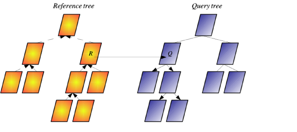
Figure 10: The solid arrows mark the flow of contribution from the reference tree to the query tree in case of a prune via a far-field to local translation between the reference node $R$ and query node $Q$. On the reference side, the far-field moments are formed in the bottom-up fashion; on the query side, the accumulated local moments will be propagated downwards during a post-processing step via local-to-local translations.

Here we consider the reference tree, which enables the consideration of the different portions of the reference set $\mathcal{R}$ at a different granularity. Given the computed far-field moments of $R^{L}$ and $R^{R}$, each centered at $R^{L}.c$ and $R^{R}.c$, how can we efficiently compute the far-field moments of $R$ centered at $R.c$, the parent of $R^{L}$ and $R^{R}$? The first operator allows the efficient bottom-up pre-computation of the Hermite moments in the reference tree.

Lemma 3.6.

Shifting a far-field expansion of a reference node to a new center (F2F translation operator for the Gaussian kernel): Given the far-field expansion centered at $R.c$ in a reference node $R$:

$$\widetilde{G}(q,\{(R,F(R.c,p))\})=\sum\limits_{\alpha<p}M_{\alpha}(R,R.c)h_{\alpha}\left(\frac{q-R.c}{\sqrt{2h^{2}}}\right)$$

this same far-field expansion shifted to a new location $c^{\prime}$ is given by:

$$\widetilde{G}(q,\{(R,F(R.c,p))\})=\widetilde{G}(q,\{(R,F(c^{\prime},p))\})=\sum\limits_{\gamma\geq 0}M_{\gamma}(R,c^{\prime})h_{\gamma}\left(\frac{q-c^{\prime}}{\sqrt{2h^{2}}}\right)$$

where

$$M_{\gamma}(R,c^{\prime})=\sum\limits_{0\leq\alpha\leq\gamma}\frac{1}{\left(\gamma-\alpha\right)!}M_{\alpha}(R,R.c)\left(\frac{R.c-c^{\prime}}{\sqrt{2h^{2}}}\right)^{\gamma-\alpha}$$ (26)

Proof.

Replace the Hermite part of the expansion by a new Taylor series:

$$\widetilde{G}(q,\{(R,F(R.c,p))\})$$

$$= \sum\limits_{\alpha<p}M_{\alpha}(R,R.c)h_{\alpha}\left(\frac{q-R.c}{\sqrt{2h^{2}}}\right)$$

$$= \sum\limits_{\alpha<p}M_{\alpha}(R,R.c)\sum\limits_{\beta\geq 0}\frac{1}{\beta!}\left(\frac{c^{\prime}-R.c}{\sqrt{2h^{2}}}\right)^{\beta}(-1)^{|\beta|}h_{\alpha+\beta}\left(\frac{q-c^{\prime}}{\sqrt{2h^{2}}}\right)$$

$$= \sum\limits_{\alpha<p}\sum\limits_{\beta\geq 0}M_{\alpha}(R,R.c)\frac{1}{\beta!}\left(\frac{c^{\prime}-R.c}{\sqrt{2h^{2}}}\right)^{\beta}(-1)^{|\beta|}h_{\alpha+\beta}\left(\frac{q-c^{\prime}}{\sqrt{2h^{2}}}\right)$$

$$= \sum\limits_{\alpha<p}\sum\limits_{\beta\geq 0}M_{\alpha}(R,R.c)\frac{1}{\beta!}\left(\frac{R.c-c^{\prime}}{\sqrt{2h^{2}}}\right)^{\beta}h_{\alpha+\beta}\left(\frac{q-c^{\prime}}{\sqrt{2h^{2}}}\right)$$

$$= \sum\limits_{\gamma<p}\left[\sum\limits_{0\leq\alpha\leq\gamma}\frac{1}{\left(\gamma-\alpha\right)!}M_{\alpha}(R,R.c)\left(\frac{R.c-c^{\prime}}{\sqrt{2h^{2}}}\right)^{\gamma-\alpha}\right]h_{\gamma}\left(\frac{q-c^{\prime}}{\sqrt{2h^{2}}}\right)$$

where $\gamma=\alpha+\beta$. ∎

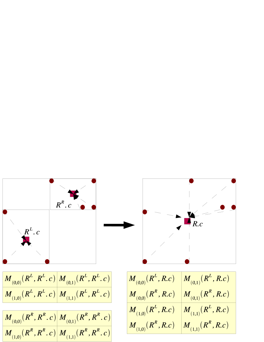
Figure 11: Given the far-field moments of $R^{L}$ and $R^{R}$ illustrated in the first two tables, Theorem 3.6 can re-center each set of far-field moments of $R^{L}$ and $R^{R}$ at centroid $R.c$. The re-centered far-field moments are shown in the third table with two numbers, each contributed by $R^{L}$ and $R^{R}$. The far-field moments of $R$ are then computed by adding up the two re-centered moments entry-wise.

Using Lemma 3.6, we can compute the far-field moments of $Q$ centered at $Q.c$ by translating the moments $\{M_{\gamma}(R^{L},R^{L}.c)\}_{\gamma<p}$ and $\{M_{\gamma}(R^{R},R^{R}.c)\}_{\gamma<p}$ to form the moments $\{M_{\gamma}(R^{L},R.c)\}_{\gamma<p}$ and $\{M_{\gamma}(R^{R},R.c)\}_{\gamma<p}$. Then, the far-field moments of $R=R_{1}\cup R_{2}$ are $\{M_{\gamma}(R^{L},R.c)+M_{\gamma}(R^{R},R.c)\}$ and

$$\widetilde{G}(q,\{(R,F(R.c,p))\})=\sum\limits_{\gamma<p}(M_{\gamma}(R^{L},R.c)+M_{\gamma}(R^{R},R.c))h_{\gamma}\left(\frac{q-R.c}{\sqrt{2h^{2}}}\right)$$

Computing each $M_{\gamma}(R^{L},R.c)$ from $M_{\gamma}(R^{L},R^{L}.c)$ (and each $M_{\gamma}(R^{R},R.c)$ from $M_{\gamma}(R^{R},R^{R}.c)$) requires iterating over at most $p^{D}$ terms. This operation runs in $O(Dp^{2D})$, which can be more efficient than computing the far-field moments of $R$ centered at $R.c$ from scratch (which is $O(|R|Dp^{D})$).

The next translation operator acts as a “clean-up” routine in a hierarchical algorithm. Since we can approximate at different scales in the query tree, we must somehow combine all the approximations at the end of the computation. By performing a breadth-first traversal of the query tree, the L2L operator shifts a node’s local expansion to the centroid of each child.

Lemma 3.7.

Shifting a combined local expansion of a query node to a new center (L2L translation operator for Gaussian kernel): Given a combined local expansion centered at $Q.c$ of the given query node $Q$:

$$\widetilde{G}(q,\mathcal{R_{D}}(Q)\cup\mathcal{R_{T}}(Q))=\sum\limits_{\beta<p}L_{\beta}(Q.c,\mathcal{R_{D}}(Q)\cup\mathcal{R_{T}}(Q))\left(\frac{q-Q.c}{\sqrt{2h^{2}}}\right)^{\beta}$$

Shifting this local expansion to the new center $c^{\prime}\in Q$ yields:

$$\widetilde{G}(q,\mathcal{R_{D}}(Q)\cup\mathcal{R_{T}}(Q))$$

$$= \sum\limits_{\alpha<p}\left[\sum\limits_{\beta\geq\alpha}\frac{\beta!}{\alpha!(\beta-\alpha)!}L_{\beta}(Q.c,\mathcal{R_{D}}(Q)\cup\mathcal{R_{T}}(Q))\left(\frac{c^{\prime}-Q.c}{\sqrt{2h^{2}}}\right)^{\beta-\alpha}\right]\left(\frac{q-c^{\prime}}{\sqrt{2h^{2}}}\right)^{\alpha}$$

where we denote

$$L_{\beta}(c^{\prime},\mathcal{R_{D}}(Q)\cup\mathcal{R_{T}}(Q))=\sum\limits_{\beta\geq\alpha}\frac{\beta!}{\alpha!(\beta-\alpha)!}L_{\beta}(Q.c,\mathcal{R_{D}}(Q)\cup\mathcal{R_{T}}(Q))\left(\frac{c^{\prime}-Q.c}{\sqrt{2h^{2}}}\right)^{\beta-\alpha}$$ (27)

Proof.

Use the multinomial theorem to expand about the new center $c^{\prime}$:

$$\widetilde{G}(q,\mathcal{R_{D}}(Q)\cup\mathcal{R_{T}}(Q))=\sum\limits_{\beta<p}L_{\beta}(Q.c,\mathcal{R_{D}}(Q)\cup\mathcal{R_{T}}(Q))\left(\frac{q-Q.c}{\sqrt{2h^{2}}}\right)^{\beta}$$

$$= \sum\limits_{\beta<p}\sum\limits_{\alpha\leq\beta}L_{\beta}(Q.c,\mathcal{R_{D}}(Q)\cup\mathcal{R_{T}}(Q))\frac{\beta!}{\alpha!(\beta-\alpha)!}\left(\frac{c^{\prime}-Q.c}{\sqrt{2h^{2}}}\right)^{\beta-\alpha}\left(\frac{q-c^{\prime}}{\sqrt{2h^{2}}}\right)^{\alpha}$$

whose summation order can be interchanged to achieve the result. ∎

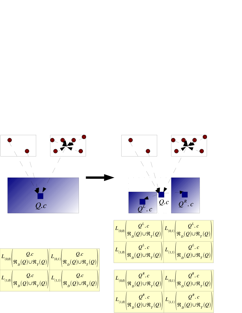
Figure 12: Given the local moments centered at $Q.c$, Theorem 3.7 can re-center them at the two centroids $Q^{L}.c$ and $Q^{R}.c$.

Using Lemma 3.7, we can shift the local moments of $Q$ centered at $Q.c$ to a different expansion center, such as an expansion center of one of the child nodes of $Q$. Let $p$ be the maximum approximation order used among the reference nodes pruned via far-to-local translation ($\mathcal{R_{T}}(Q)$) and direct local accumulation ($\mathcal{R_{D}}(Q)$). The local moment propagation to both child nodes of $Q$ is achieved by the following operations:

$$\{L_{\beta}(Q^{L}.c,\mathcal{R_{D}}(Q^{L})\cup\mathcal{R_{T}}(Q^{L}))\}_{\beta<p}\leftarrow \{L_{\beta}(Q^{L}.c,\mathcal{R_{D}}(Q^{L})\cup\mathcal{R_{T}}(Q^{L}))\}_{\beta<p}+$$

$$\{L_{\beta}(Q^{L}.c,\mathcal{R_{D}}(Q)\cup\mathcal{R_{T}}(Q))\}_{\beta<p}$$

$$\{L_{\beta}(Q^{R}.c,\mathcal{R_{D}}(Q^{R})\cup\mathcal{R_{T}}(Q^{R}))\}_{\beta<p}\leftarrow \{L_{\beta}(Q^{R}.c,\mathcal{R_{D}}(Q^{R})\cup\mathcal{R_{T}}(Q^{R}))\}_{\beta<p}+$$

$$\{L_{\beta}(Q^{L}.c,\mathcal{R_{D}}(Q)\cup\mathcal{R_{T}}(Q))\}_{\beta<p}$$

where the addition operation is an element-wise operation that combines the two scalars with the same multi-index position.

3.8 Choosing the Best Approximation Method

Suppose we are given a query node $Q$ and a reference node $R$ pair during the invocation of Algorithm 13. CanSummarize function for the higher-order DFGT algorithm has four approximation methods available: $A\in\{E,T(c,p),F(c,p),$ $D(c,p)\}$ (see Section 3.2). Because we would like to avoid exhaustive computations, the higher-order DFGT algorithm uses only three of the approximation methods and defers exhaustive computations until query/reference leaf pairs are encountered. Algorithm 7 tests whether the given query node and reference node pair can be approximated by evaluating the far-field moments of $R$, computing direct local accumulation due to $R$, and translating some of the terms that constitute the far-field moments of $R$ (far-field-to-local translation operator) and evaluates the asymptotic cost of each approximation. Algorithm 7 then determines the approximation method with the lowest asymptotic cost. This idea was originally introduced in [11] in the description of the original fast Gauss transform algorithm. The key difference is that even if Algorithm 7 returns $E$ (when none of the other approximation methods can beat the cost of the exhaustive method), our hierarchical algorithm will not default to exhaustive evaluations and will consider the query points and reference points at a finer granularity, as shown in Algorithm 13.

Algorithm 7 $\mbox{{ChooseBestMethod}}(Q,R,\tau)$: Chooses the FMM-type approximation with the least cost for a query and reference node pair.

  $p_{F}\leftarrow\textsc{FarFieldOrder}(Q,R,\tau)$

  $p_{D}\leftarrow\textsc{LocalAccumulationOrder}(Q,R,\tau)$

  $p_{T}\leftarrow\textsc{ConvertFarFieldToLocalOrder}(Q,R,\tau)$

  $c_{F}\leftarrow N_{Q}D^{p_{F}+1}$, $c_{D}\leftarrow N_{R}D^{p_{D}+1}$, $c_{T}\leftarrow D^{2p_{T}+1}$, $c_{E}\leftarrow DN_{Q}N_{R}$

  if $c_{F}=\min\{c_{F},c_{D},c_{T},c_{E}\}$ then

     return  $F(R.c,p_{F})$

  else if $c_{D}=\min\{c_{F},c_{D},c_{T},c_{E}\}$ then

     return  $D(Q.c,p_{D})$

  else if $c_{T}=\min\{c_{F},c_{D},c_{T},c_{E}\}$ then

     return  $T(Q.c,p_{T})$

  else

     return  $E$

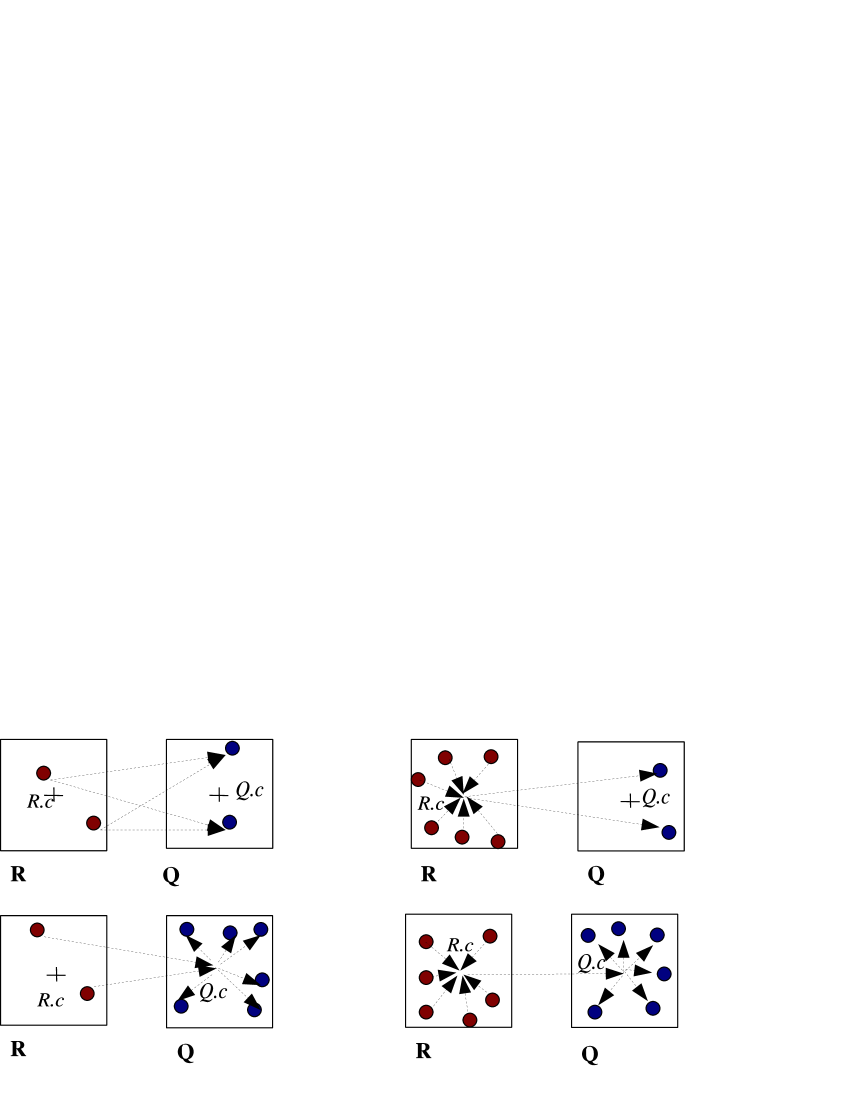
Figure 13: Four ways of approximating the contribution of a reference node to a query node. Top left: exhaustive computations (few reference points/few query points); Top right: far-field moment evaluating (many reference points/few query points); Bottom left: direct local moment accumulation (few reference points/many query points); Bottom right: far-field-to-local translation (many reference points/many query points).

3.9 Hierarchical FGT

Given the analytical machinery developed in the previous section, we now describe how to extend the centroid-based dual-tree [7, 9] to do higher-order approximations. The main structure of the algorithm is shown in Algorithm 8. We provide only a high-level overview of our algorithm and defer the discussion on the implementation details to Appendix.

Algorithm 8 $\mbox{{DFGTMain}}(\mathcal{Q},\mathcal{R})$: The main KDE routine.

  $Q^{\mathit{root}}\leftarrow\textsc{BuildKdTree}(\mathcal{Q})$,       $R^{\mathit{root}}\leftarrow\textsc{BuildKdTree}(\mathcal{R})$

  $\mbox{{DFGTInitQ}}(Q^{\mathit{root}})$,       $\mbox{{DFGTInitR}}(R^{\mathit{root}})$

   $\mbox{{DFGT}}(Q^{\mathit{root}},R^{\mathit{root}})$,       $\mbox{{DFGTPost}}(Q^{\mathit{root}})$

Initialization of the query tree. Each query node maintains a vector storing $\left(p_{\mathit{max}}\right)^{D}$ terms, where $p_{\mathit{max}}$ is a pre-determined limit on the approximation order depending on the dimensionality of the query set $\mathcal{Q}$ and the reference set $\mathcal{R}$. For the experimental results, we have fixed $p_{\mathit{max}}=6$ for $D=2$, $p_{\mathit{max}}=4$ for $D=3$, $p_{\mathit{max}}=2$ for $D=4$ and $D=5$, $p_{\mathit{max}}=1$ for $D\geq 6$.

Algorithm 9 $\mbox{{DFGTInitQ}}(Q)$: Initializes query bound summary statistics.

  {Initialize the node bound summary statistics.}

  $G^{l}(Q,\mathcal{R})\leftarrow 0$,    $G^{u}(Q,\mathcal{R})\leftarrow|\mathcal{R}|$,    $Q.\Delta^{l}\leftarrow 0$,    $Q.\Delta^{u}\leftarrow 0$

  {Initialize translated local moments to be a vector of length $\left(p_{\mathit{max}}^{D}\right)$.}

  $Q.L_{0\leq i<\left(p_{\mathit{max}}\right)^{D}}\leftarrow 0$

  if $Q$ is a leaf node then

     {Initialize for each query point.}

     for each $q_{i_{m}}\in Q$ do

        $G^{l}(q_{i_{m}},\mathcal{R})\leftarrow 0$,       $G^{u}(q_{i_{m}},\mathcal{R})\leftarrow|\mathcal{R}|$

         $\widetilde{G}(q_{i_{m}},\mathcal{R})\leftarrow 0$,       $\widetilde{G}(q_{i_{m}},\mathcal{R_{E}}(q_{i_{m}}))\leftarrow 0$

        $\widetilde{G}(q_{i_{m}},\mathcal{R_{F}}(q_{i_{m}}))\leftarrow 0$,       $\widetilde{G}(q_{i_{m}},\mathcal{R_{D}}(q_{i_{m}})\cup\mathcal{R_{T}}(q_{i_{m}}))\leftarrow 0$

  else

      $\mbox{{DFGTInitQ}}(Q^{L})$,       $\mbox{{DFGTInitQ}}(Q^{R})$

Pre-computation of far-field moments. Before the main KDE computation can begin, we pre-compute the far-field moments of each reference node in the reference tree up to $\left(p_{\mathit{max}}\right)^{D}$ terms. We show how to efficiently pre-compute the far-field moments of each reference node in the reference tree in Algorithm 10. The algorithm uses Equation (20) for the leaf node and Equation (26) for translating the moments of the child nodes for the internal node case. We describe the implementation details in Appendix.

Algorithm 10 $\mbox{{DFGTInitR}}(R)$: Pre-computes far-field moments.

  {Initialize the far-field moments of $R$ to be empty.}

  for $i=0$ to $i<(p_{\mathit{max}})^{D}$ do

     $M_{\mbox{{PositionToMultiindex}}(i,p_{\mathit{max}})}(R,R.c)\leftarrow 0$

  if $R$ is a leaf node then

     {Accumulate far-field moment from each point (Equation (20)).}

     $\mbox{{AccumulateFarFieldMoment}}(R)$

  else

     {Recursively compute the moments of the child nodes and combine them.}

     $\mbox{{DFGTInitR}}(R^{L})$,       $\mbox{{DFGTInitR}}(R^{R})$

     $\mbox{{TransFarToFar}}(R^{L},R)$,       $\mbox{{TransFarToFar}}(R^{R},R)$

Determining the prunability of the given query and reference pair (shown in Algorithm 12). Note that the function Summarize includes calls to the following functions (see Appendix):

1. EvalFarFieldExpansion: evaluates the far-field moments stored in $R$ at each query point in $Q$ up to $(p_{F})^{D}$ terms. See Algorithm 23.

2. AccumulateDirectLocalMoment: computes direct local moment contribution of $R$ centered at $Q.c$ in $Q$. See Algorithm 25.

3. TransFarToLocal: translates the far-field moments of $R$ up to $(p_{T})^{D}$ terms to the local moment centered $Q.c$ in $Q$. See Algorithm 24.

Algorithm 11 $\mbox{{CanSummarize}}(Q,R,\epsilon)$: Determines the prunability of the given query node $Q$ and reference node $R$

  return  $\mbox{{ChooseBestMethod}}\left(Q,R,\frac{\epsilon|R|G^{l,\mathit{new}}(Q,\mathcal{R})}{|\mathcal{R}|}\right)\not=E$

Algorithm 12 $\mbox{{Summarize}}(Q,R)$: Summarizes the contribution of $R$.

  {Add bound changes.}

  $Q.\Delta^{l}\leftarrow Q.\Delta^{l}+\delta^{l}(Q,R)$, $Q.\Delta^{u}\leftarrow Q.\Delta^{u}+\delta^{u}(Q,R)$

  if $A$ is of the form $F(R.c,p_{F})$ then

     $\mbox{{EvalFarFieldExpansion}}(R,Q,p_{F})$

  else if $A$ is of the form $D(Q.c,p_{D})$ then

     $\mbox{{AccumulateDirectLocalMoment}}(R,Q,p_{D})$

  else

     $\mbox{{TransFarToLocal}}(R,Q,p_{T})$

Algorithm 13 $\mbox{{DFGT}}(Q,R)$: The core dual-tree routine for computing KDE.

  $\delta^{l}(Q,R)=|R|K_{h}(d^{u}(Q,R))$, $\delta^{u}(Q,R)=|R|(K_{h}(d^{l}(Q,R))-1)$

  {Add postponed contributions/bound changes from the current pair.}

  $G^{l,\mathit{new}}(Q,\mathcal{R})\leftarrow G^{l}(Q,\mathcal{R})+Q.\Delta^{l}+\delta^{l}(Q,R)$

  $G^{u,\mathit{new}}(Q,\mathcal{R})\leftarrow G^{u}(Q,\mathcal{R})+Q.\Delta^{u}+\delta^{u}(Q,R)$

  if $\mbox{{CanSummarize}}(Q,R,\epsilon)$ then

     $\mbox{{Summarize}}(Q,R)$

  else

     if $Q$ is a leaf node then

        if $R$ is a leaf node then

           $\mbox{{DFGTBase}}(Q,R)$

        else

           $\mbox{{DFGT}}(Q,R^{L})$,$\mbox{{DFGT}}(Q,R^{R})$

     else

        {Push down postponed bound changes owned by $Q$ to the children.}

        $Q^{L}.\Delta^{l}\leftarrow Q^{L}.\Delta^{l}+Q.\Delta^{l}$,      $Q^{R}.\Delta^{l}\leftarrow Q^{R}.\Delta^{l}+Q.\Delta^{l}$

        $Q^{L}.\Delta^{u}\leftarrow Q^{L}.\Delta^{u}+Q.\Delta^{u}$,      $Q^{R}.\Delta^{u}\leftarrow Q^{R}.\Delta^{u}+Q.\Delta^{u}$

        $Q.\Delta^{l}\leftarrow 0$,      $Q.\Delta^{u}\leftarrow 0$

        if $R$ is a leaf node then

           $\mbox{{DFGT}}(Q^{L},R)$, $\mbox{{DFGT}}(Q^{R},R)$

        else

           $\mbox{{DFGT}}(Q^{L},R^{L})$,$\mbox{{DFGT}}(Q^{L},R^{R})$,$\mbox{{DFGT}}(Q^{R},R^{L})$,$\mbox{{DFGT}}(Q^{R},R^{R})$

        {Refine the bounds based on the recursion results.}

        $G^{l}(Q,\mathcal{R})\leftarrow\min\{G^{l}(Q^{L},\mathcal{R})+Q^{L}.\Delta^{l},G^{l}(Q^{R},\mathcal{R})+Q^{R}.\Delta^{l}\}$

        $G^{u}(Q,\mathcal{R})\leftarrow\max\{G^{u}(Q^{L},\mathcal{R})+Q^{L}.\Delta^{u},G^{u}(Q^{R},\mathcal{R})+Q^{R}.\Delta^{u}\}$

Dual-tree Recursion. Algorithm 13 shows the basic structure of the dual-tree based KDE computation (see Figure 4). This procedure is first called with $Q$ and $R$ as the root nodes of the query and the reference tree respectively. CanSummarize takes three parameters: the current query node $Q$, the current reference node $R$, and the global relative error tolerance $\epsilon$. This function tests whether the the contribution of the given reference node for each query point in the given query node can be approximated within the error tolerance. If the approximation is not possible, then the algorithm continues to consider the query and the reference data at a finer granularity. The basic idea is to terminate the recursion as soon as possible by considering large “chunks” of the query data and the reference data and avoiding the number of exhaustive leaf-leaf computations. We can achieve this if we utilize approximation schemes that yield high accuracy and have cheap computational costs.

Each prune made for a pair of a query and a reference node is summarized in the given query node by incorporating the lower and the upper bound changes $\delta^{l}(Q,R)$ and $\delta^{u}(Q,R)$ contributed by the reference node into $Q.\Delta^{l}$ and $Q.\Delta^{u}$. These two bound updates due to a prune can be regarded as a new piece of information which is known only locally to the given query node $Q$. All of the bounds in the entire subtree of $Q$ should reflect this information. One way to achieve this effect is to pass the lower bound and the upper bound changes owned by $Q$ (i.e., $Q.\Delta^{l}$ and $Q.\Delta^{u}$) to $Q$’s immediate children, whenever the algorithm needs to consider the query dataset at a finer granularity by recursing to the left and the right child of $Q$.

Algorithm 14 $\mbox{{DFGTBase}}(Q,R)$: Computes exact contribution of $R$ to $Q$.

  $G^{l}(Q,\mathcal{R})\leftarrow\infty$,       $G^{u}(Q,\mathcal{R})\leftarrow-\infty$

  for each $q_{i_{m}}\in Q$ do

     {Add postponed changes passed down from the ancestor node of $Q$.}

     $G^{l}(q_{i_{m}},\mathcal{R})\leftarrow G^{l}(q_{i_{m}},\mathcal{R})+Q.\Delta^{l}$,       $G^{u}(q_{i_{m}},\mathcal{R})\leftarrow G^{u}(q_{i_{m}},\mathcal{R})+Q.\Delta^{u}$

     for each $r_{j_{n}}\in R$ do

        $v\leftarrow K_{h}(\|q_{i_{m}}-r_{j_{n}}\|)$,         $G^{l}(q_{i_{m}},\mathcal{R})\leftarrow G^{l}(q_{i_{m}},\mathcal{R})+v$

        $\widetilde{G}(q_{i_{m}},\mathcal{R_{E}}(q_{i_{m}}))\leftarrow\widetilde{G}(q_{i_{m}},\mathcal{R_{E}}(q_{i_{m}}))+v$

        $G^{u}(q_{i_{m}},\mathcal{R})\leftarrow G^{u}(q_{i_{m}},\mathcal{R})+(v-1)$

     {Refine the bound summary statistics owned by $Q$.}

     $G^{l}(Q,\mathcal{R})\leftarrow\min\{G^{l}(Q,\mathcal{R}),G^{l}(q_{i_{m}},\mathcal{R})\}$

     $G^{u}(Q,\mathcal{R})\leftarrow\max\{G^{u}(Q,\mathcal{R}),G^{u}(q_{i_{m}},\mathcal{R})\}$

  $Q.\Delta^{l}\leftarrow 0$,       $Q.\Delta^{u}\leftarrow 0$

Base-case Computation. If a given leaf query and leaf reference node pair could not be pruned, then DFGTBase (shown in Algorithm 14) is called. Because all kernel evaluations are computed exactly, we can refine the bound summary statistics of the given query node $Q$ (that is, $G^{l}(Q,\mathcal{R})$ and $G^{u}(Q,\mathcal{R})$) further and hence we reset them to $\infty$ and $-\infty$ respectively. For each query point $q_{i_{m}}\in Q$, we first incorporate the postponed bound changes passed down from the ancestor node of $Q$. We loop over each reference point $r_{j_{n}}\in R$ and compute the kernel value between $q_{i_{m}}$ and $r_{j_{n}}$ and accumulate the lower bound $G^{l}(q_{i_{m}},\mathcal{R})$, the kernel sum computed exhaustively $\widetilde{G}(q_{i_{m}},\mathcal{R_{E}}(q_{i_{m}}))$, and the upper bound $G^{u}(q_{i_{m}},\mathcal{R})$

Note that we subtract one for updating $G^{u}(q_{i_{m}},\mathcal{R})$ for correcting the prior assumption that $K_{h}(||q_{i_{m}}-r_{j_{n}}||)=1$, while the lower bound $G^{l}(q_{i_{m}},\mathcal{R})$ and $\widetilde{G}(q_{i_{m}},\mathcal{R_{E}}(q_{i_{m}}))$ are incremented by $K_{h}(||q_{i_{m}}-r_{j_{n}}||)$. As the contribution of the reference node $R$ is added onto the query point $q_{i_{m}}$’s sum, we can refine the bound summary statistics owned by $Q$ such that $G^{l}(Q,\mathcal{R})=\min\limits_{q_{i_{m}}\in Q}G^{l}(q_{i_{m}},\mathcal{R})$ and $G^{u}(Q,\mathcal{R})=\max\limits_{q_{i_{m}}\in Q}G^{u}(q_{i_{m}},\mathcal{R})$. Finally, we reset the postponed bound changes stored in $Q$ to zero.

Post-processing (shown in Algorithm 15). For the non-leaf case, the local-to-local translation operator (TransLocalToLocal) is called to re-center the local moments at the current level and passes them down to the child nodes. For the leaf-case, EvalLocalExpansion is called to convert local moments to a single scalar that represents the contribution to a given query point.

Algorithm 15 $\mbox{{DFGTPost}}(Q)$: The post-processing routine.

  if $Q$ is a leaf node then

     $G^{l}(Q,\mathcal{R})\leftarrow\infty$,       $G^{u}(Q,\mathcal{R})\leftarrow-\infty$

     for each $q_{i_{m}}\in Q$ do

        {Add bound changes for the query node at the given query point $q_{i_{m}}$.}

        $G^{l}(q_{i_{m}},\mathcal{R})\leftarrow G^{l}(q_{i_{m}},\mathcal{R})+Q.\Delta^{l}$,     $G^{u}(q_{i_{m}},\mathcal{R})\leftarrow G^{u}(q_{i_{m}},\mathcal{R})+Q.\Delta^{u}$

        {Refine summary statistics for lower and upper bounds.}

        $G^{l}(Q,\mathcal{R})\leftarrow\min\{G^{l}(Q,\mathcal{R}),G^{l}(q_{i_{m}},\mathcal{R})\}$

        $G^{u}(Q,\mathcal{R})\leftarrow\max\{G^{u}(Q,\mathcal{R}),G^{u}(q_{i_{m}},\mathcal{R})\}$

        {Compute the contributions from the accumulated local moments.}

        $\widetilde{G}(q_{i_{m}},\mathcal{R_{T}}(q_{i_{m}}))\leftarrow\mbox{{EvalLocalExpansion}}(Q)$

        {Sum the contribution from the local moments (direct or translated), the far-field evaluations, and exhaustive evaluations.}

        $\widetilde{G}(q_{i_{m}},\mathcal{R})\leftarrow\widetilde{G}(q_{i_{m}},\mathcal{R_{D}}(q_{i_{m}})\cup\mathcal{R_{T}}(q_{i_{m}}))+\widetilde{G}(q_{i_{m}},\mathcal{R_{F}}(q_{i_{m}}))+\widetilde{G}(q_{i_{m}},\mathcal{R_{E}})$

     $\Delta^{l}(Q)\leftarrow 0$,     $\Delta^{u}(Q)\leftarrow 0$,     $Q.L\leftarrow 0$

  else

     $\mbox{{TransLocalToLocal}}(Q,Q^{L})$,       $\mbox{{TransLocalToLocal}}(Q,Q^{R})$

     $Q^{L}.\Delta^{l}\leftarrow Q^{L}.\Delta^{l}+Q.\Delta^{l}$,     $Q^{R}.\Delta^{l}\leftarrow Q^{R}.\Delta^{l}+Q.\Delta^{l}$

     $Q^{L}.\Delta^{u}\leftarrow Q^{L}.\Delta^{u}+Q.\Delta^{u}$,     $Q^{R}.\Delta^{u}\leftarrow Q^{R}.\Delta^{u}+Q.\Delta^{u}$

     $Q.L\leftarrow 0$,     $Q.\Delta^{l}\leftarrow 0$,     $Q.\Delta^{u}\leftarrow 0$

     $\mbox{{DFGTPost}}(Q^{L})$,     $\mbox{{DFGTPost}}(Q^{R})$

     {Refine the bounds based on the results of the recursion.}

     $G^{l}(Q,\mathcal{R})\leftarrow\min\{G^{l}(Q^{L},\mathcal{R}),G^{l}(Q^{R},\mathcal{R})\}$

     $G^{u}(Q,\mathcal{R})\leftarrow\max\{G^{u}(Q^{L},\mathcal{R}),G^{u}(Q^{R},\mathcal{R})\}$

3.10 Basic Properties of DFGT Algorithms

Theorem 3.8.

Lower/upper bounds are maintained properly at all times for each $q\in\mathcal{Q}$ and each query node $Q$ during the function call DFGTMain.

Proof.

We show that the bounds are maintained properly for three main parts in the function DFGTMain: DFGTInitQ, DFGT, and DFGTPost.

The function call DFGTInitQ: It is clear that for all $q_{i}\in\mathcal{Q}$, $0=G^{l}(q_{i},\mathcal{R})\leq G(q_{i},\mathcal{R})\leq G^{u}(q_{i},\mathcal{R})=|\mathcal{R}|$. Furthermore, for each query node $Q$, $0=G^{l}(Q,\mathcal{R})\leq G(q_{i_{m}},\mathcal{R})\leq G^{u}(Q,\mathcal{R})=|\mathcal{R}|$ for each $q_{i_{m}}\in Q$.

The function call DFGTBase: Let $Q$ and $R$ be the query node and the reference node respectively. For each query point $q_{i_{m}}\in Q$, $G^{l}(q_{i_{m}},\mathcal{R})$ is incremented by $Q.\Delta^{l}+\sum\limits_{r_{j_{n}}\in R}K_{h}(||q_{i_{m}}-r_{j_{n}}||)$, and $G^{u}(q_{i_{m}},\mathcal{R})$ by $Q.\Delta^{u}+$

$\sum\limits_{r_{j_{n}}\in R}\left(K_{h}(||q_{i_{m}}-r_{j_{n}}||)-1\right)$; this operation incorporates the passed-down contribution for $q_{i_{m}}\in Q$, and un-does the assumption made during the initialization phase of DFGTInitQ. $G^{l}(Q,\mathcal{R})$ and $G^{u}(Q,\mathcal{R})$ are updated to be the minimum among $G^{l}(q_{i_{m}},\mathcal{R})$ and the maximum among $G^{u}(q_{i_{m}},\mathcal{R})$ respectively. The postponed bound changes $Q.\Delta^{l}$ and $Q.\Delta^{u}$ are cleared to avoid double-counting when $Q$ may be visited later.

The function call DFGT: We induct on the number of points owned by the query node $Q$ and the reference node $R$ in consideration (i.e. $|Q|+|R|$). The only possible places that change $G^{l}(q_{i_{m}},\mathcal{R})$, $G^{u}(q_{i_{m}},\mathcal{R})$, $G^{l}(Q,\mathcal{R})$ and $G^{u}(Q,\mathcal{R})$ are the call to the base case function DFGTBase and the last two lines of the function DFGT. The correctness of DFGTBase function is proven already, so we consider the second case. The two function calls $\mbox{{DFGT}}(Q^{L},R)$ and $\mbox{{DFGT}}(Q^{R},R)$ (in case $R$ is a leaf node) and the four function calls
$\mbox{{DFGT}}(Q^{L},R^{L})$, $\mbox{{DFGT}}(Q^{L},R^{R})$, $\mbox{{DFGT}}(Q^{R},R^{L})$, and $\mbox{{DFGT}}(Q^{R},R^{R})$ (in case $R$ is an internal node) are smaller subproblems than $(Q,R)$ pair. By the induction hypothesis, these calls maintain the lower and the upper bounds properly. The lower bound is set to the minimum of the “best” lower bound owned by the children of $Q$: $\min\{G^{l}(Q^{L},\mathcal{R})+Q^{L}.\Delta^{l},G^{l}(Q^{R},\mathcal{R})+Q^{R}.\Delta^{l}\}$. Similarly, the upper bound is set to the maximum of the “best” upper bound owned by the children of $Q$: $\max\{G^{u}(Q^{L},\mathcal{R})+Q^{L}.\Delta^{u},G^{u}(Q^{R},\mathcal{R})+Q^{R}.\Delta^{u}\}$.

The function call DFGTPost: We again induct on the number of points owned by the query node $Q$ passed in as the argument to this function. If the query node $Q$ is a leaf node, each query point $q_{i_{m}}\in Q$ incorporates the passed-down bound changes $Q.\Delta^{l}$ and $Q.\Delta^{u}$. The bounds $G^{l}(Q,\mathcal{R})$ and $G^{u}(Q,\mathcal{R})$ are (correctly) set to the minimum among $G^{l}(q_{i_{m}},\mathcal{R})$ and the maximum among $G^{u}(q_{i_{m}},\mathcal{R})$. If $Q$ is not a leaf node: we know the sub-calls $\mbox{{DFGTPost}}(Q^{L})$ and $\mbox{{DFGTPost}}(Q^{R})$ maintains correct lower and upper bounds by the induction hypothesis since $Q^{L}$ and $Q^{R}$ contain a smaller number of points. Setting the lower and upper bounds for $Q$ by the operations: $G^{l}(Q,\mathcal{R})\leftarrow\min\{G^{l}(Q^{L},\mathcal{R}),G^{l}(Q^{R},\mathcal{R})\}$, $G^{u}(Q,\mathcal{R})\leftarrow\max\{G^{u}(Q^{L},\mathcal{R}),G^{u}(Q^{R},\mathcal{R})\}$ is valid. ∎

Theorem 3.9.

After calling DFGTPost (Algorithm 15) in DFGTMain (Algorithm 8), each query point $q_{i}\in\mathcal{Q}$ accounts for every reference point $r_{j}\in\mathcal{R}$ in its Gaussian kernel sum approximation $\widetilde{G}(q_{i},\mathcal{R})$.

Proof.

In Algorithm 13, for each $q_{i}\in\mathcal{Q}$, each $r_{j}\in\mathcal{R}$ is either accounted by an exhaustive computation in DFGTBase or a prune in Summarize. All exhaustive computations for $q_{i}\in Q$ directly update $\widetilde{G}(q_{i},\mathcal{R_{E}}(q_{i}))$, while any pruned contributions will be incorporated into each $\widetilde{G}(q_{i},\mathcal{R_{T}}(q_{i}))$ (hence into $\widetilde{G}(q_{i},\mathcal{R}(q_{i}))$) and when they are pushed down (to the leaf node to which $q_{i}$ belongs) during the DFGT recursion or DFGTPost. ∎

Theorem 3.10.

For each query point $q_{i}\in\mathcal{Q}$, the approximated kernel sum $\widetilde{G}(q_{i},\mathcal{R})$ satisfies the global relative error tolerance $\epsilon$.

Proof.

For simplicity, let us limit the available approximation methods to $A\in\{E,T(c,1)\}$ where $E$ denotes the exhaustive computation and $T(c,1)$ denotes the centroid-based approximation about $c$.

Given $q_{i}\in\mathcal{Q}$, let $Q^{\prime}$ be the (unique) leaf node that owns $q_{i}$. Let $\{R_{T_{a}}\}_{a=1}^{N_{a}}$ denote the set of reference nodes whose kernel sum contribution were accounted via centroid approximation and $\{R_{E_{b}}\}_{b=1}^{N_{b}}$ the set of reference nodes whose kernel sum contribution were computed exhaustively. Then it is clear that $\mathcal{R}=\left(\bigcup\limits_{a=1}^{N_{a}}R_{T_{a}}\right)\cup\left(\bigcup\limits_{b=1}^{N_{b}}R_{E_{b}}\right)$ with $R_{T_{a^{\prime}}}\cap R_{T_{a^{\prime\prime}}}=\emptyset$, $R_{E_{b^{\prime}}}\cap R_{E_{b^{\prime\prime}}}=\emptyset$, $R_{T_{a^{\prime}}}\cap R_{E_{b^{\prime}}}=\emptyset$ for $1\leq a^{\prime},a^{\prime\prime}\leq N_{a}$ and $1\leq b^{\prime},b^{\prime\prime}\leq N_{b}$. Let $Q_{T_{a}}$ be the query node that owns $q_{i}$ and is considered with the reference node $R_{T_{a}}$ and pruned. Let $G^{l(a)}(Q_{T_{a}},\mathcal{R})$ be a “snapshot” of the running lower bound on the kernel sum for query points owned by $Q_{T_{a}}$ at the time the query node $Q_{T_{a}}$ and the reference node $R_{T_{a}}$ were considered (and subsequently pruned). By the triangle inequality:

$$\left|\widetilde{G}(q_{i},\mathcal{R})-G(q_{i},\mathcal{R})\right|$$

$$= \Biggl{|}\widetilde{G}\left(q_{i},\left(\bigcup\limits_{a=1}^{N_{a}}\left\{(R_{T_{a}},T(Q.c,1))\right\}\right)\cup\left(\bigcup\limits_{b=1}^{N_{b}}\left\{(R_{E_{b}},E)\right\}\right)\right)-$$

$$G\left(q_{i},\left(\bigcup\limits_{a=1}^{N_{a}}R_{T_{a}}\right)\cup\left(\bigcup\limits_{b=1}^{N_{b}}R_{E_{b}}\right)\right)\Biggr{|}$$

$$\leq \Biggl{|}\left(\sum\limits_{a=1}^{N_{a}}\widetilde{G}\left(q_{i},\{(R_{T_{a}},T(Q.c,1))\}\right)-G(q_{i},R_{T_{a}})\right)+$$

$$\left(\sum\limits_{b=1}^{N_{b}}\widetilde{G}\left(q_{i},\{(R_{E_{b}},E)\}\right)-G(q_{i},R_{E_{b}})\right)\Biggr{|}$$

$$\leq \sum\limits_{a=1}^{N_{a}}\left|\widetilde{G}\left(q_{i},\{(R_{T_{a}},T(Q.c,1))\}\right)-G(q_{i},R_{T_{a}})\right|+\sum\limits_{b=1}^{N_{b}}\left|\widetilde{G}\left(q_{i},\{(R_{E_{b}},E)\}\right)-G(q_{i},R_{E_{b}})\right|$$

$$\leq \sum\limits_{a=1}^{N_{a}}|R_{T_{a}}|\max\left\{\begin{array}[]{c}\left|K_{h}(d^{u}(Q_{T_{a}},R_{T_{a}}))-K_{h}(||Q_{T_{a}}.c-R_{T_{a}}.c||)\right|,\\ \left|K_{h}(d^{l}(Q_{T_{a}},R_{T_{a}}))-K_{h}(||Q_{T_{a}}.c-R_{T_{a}}.c||)\right|\end{array}\right\}+\sum\limits_{b=1}^{N_{b}}|R_{E_{b}}|\cdot 0$$

$$\leq \sum\limits_{a=1}^{N_{a}}\frac{|R_{T_{a}}|\epsilon}{|\mathcal{R}|}G^{l(a)}(Q_{T_{a}},\mathcal{R})+\sum\limits_{b=1}^{N_{b}}\frac{|R_{E_{b}}|\epsilon}{|\mathcal{R}|}G^{l(b)}(Q^{\prime},\mathcal{R})$$

$$\leq \sum\limits_{a=1}^{N_{a}}\frac{|R_{T_{a}}|\epsilon}{|\mathcal{R}|}G(q_{i},\mathcal{R})+\sum\limits_{b=1}^{N_{b}}\frac{|R_{E_{b}}|\epsilon}{|\mathcal{R}|}G(q_{i},\mathcal{R})\leq\epsilon G(q_{i},\mathcal{R})$$

The proof can be easily extended to the case with four available approximation methods $A\in\{E,T(c,p),F(c,p),D(c,p)\}$. ∎

Alg$\backslash$Scale	0.001	0.01	0.1	1	10	100	1000	$\Sigma$
sj2-50000-2, $D=2,N=50000,h_{CV_{LS}}^{*}=0.00139506$
Naive	241	241	241	241	241	241	241	1687
FFT	$\infty$	$\infty$	$\infty$	$\infty$	$\infty$	1.02	0.03	$\infty$
FGT	X	X	X	2.63	1.48	0.33	0.18	X
IFGT	$\infty$	$\infty$	$\infty$	155	7.26	0.40	0.03	$\infty$
DFD	1.58	1.63	2.14	4.33	39.7	29.5	1.51	80.39
DFGT	0.43	0.47	1.00	3.48	21	2.48	0.96	29.8
colors50k, $D=2,N=50000,h_{CV_{LS}}^{*}=0.0016911$
Naive	241	241	241	241	241	241	241	1687
FFT	$\infty$	$\infty$	$\infty$	$\infty$	$\infty$	$\infty$	0.16	$\infty$
FGT	X	X	X	120	10	4	0.22	X
IFGT	$\infty$	$\infty$	$\infty$	$\infty$	$\infty$	0.54	0.07	$\infty$
DFD	1.62	1.76	2.36	12.5	102	17.0	2.41	139.65
DFGT	0.44	0.60	1.21	15.6	20	4.20	0.67	42.7
bio5, $D=5,N=103010,h_{CV_{LS}}^{*}=0.000308646$
Naive	1310	1310	1310	1310	1310	1310	1310	9170
FFT	X	X	X	X	X	X	X	X
FGT	X	X	X	X	X	X	X	X
IFGT	$\infty$	$\infty$	$\infty$	$\infty$	$\infty$	$\infty$	1.04	$\infty$
DFD	0.34	0.36	0.92	6.31	113	643	125	888.93
DFGT	0.35	0.37	0.94	6.51	102	304	121	535.17

Figure 14: Empirical comparison of six different algorithms on different magnitudes of bandwidths on three different datasets. Each entry in the table has a timing number (if finite), $\infty$ symbol (if no parameter tweaking could achieve the error tolerance), $X$ symbol (if the algorithm segfaulted).

4 Experimental Results

We evaluated empirical performance of six algorithms:

• Naive: the brute-force algorithm (Algorithm 1).

• FFT: Fast fourier transform based kernel density estimate [18].

• FGT: Fast Gauss transform [11].

• IFGT: improved fast Gauss transform [19, 13].

• DFD: the dual-tree centroid-based approximation method [7, 9].

• DFGT: our new algorithm (Algorithm 8).

Alg$\backslash$Scale	0.001	0.01	0.1	1	10	100	1000	$\Sigma$
edsgc-radec, $D=2,N=1495877,h_{CV_{LS}}^{*}=0.000473061$
Naive	2.2e5	2.2e5	2.2e5	2.2e5	2.2e5	2.2e5	2.2e5	1.5e6
DFD	4.9e1	4.9e1	6.3e1	1e2	1.5e3	2e4	1.3e3	2.3e4
DFGT	6.8e0	7.4e0	2.1e1	5.9e1	1.7e3	3.5e3	1.4e2	5.4e3
mockgalaxy-D-1M, $D=3,N=1000000,h_{CV_{LS}}^{*}=0.00010681$
Naive	9.6e4	9.6e4	9.6e4	9.6e4	9.6e4	9.6e4	9.6e4	6.7e5
DFD	2.4e0	2.4e0	2.6e0	1.5e1	9.7e1	1.7e2	4.4e3	4.7e3
DFGT	2.4e0	2.4e0	2.6e0	1.5e1	1.1e2	2.1e2	4e3	4.3e3
psf1-psf4-stargal-2d-only, $D=2,N=3056092,h_{CV_{LS}}^{*}=0.00489463$
Naive	9e5	9e5	9e5	9e5	9e5	9e5	9e5	6.3e6
DFD	1.1e2	1.5e2	1.2e3	2.2e4	3.9e4	2.9e3	1.1e2	6.5e4
DFGT	3.9e1	8.1e1	1.4e3	1.6e4	2.3e3	1.9e2	4.2e1	1.9e4

Figure 15: Empirical comparison of three algorithms on different magnitudes of bandwidths on three larger datasets. All timings are reported in seconds.

We used the following six real-world datasets:

• sj2-50000-2: two-dimensional astronomy position dataset.

• colors50k: two-dimensional astronomy color dataset.

• bio5: five-dimensional pharmaceutical dataset.

• edgsc-radec: two-dimensional astronomy angle dataset.

• mockgalaxy-D-1M: three-dimensional astronomy position dataset.

• psf1-psf4-stargal-2d-only: two-dimensional astronomy dataset.

Note that the last three datasets contain over 1 million points and demonstrate the scalability of our fast algorithm. For each dataset, we evaluated the empirical performance on computing kernel density estimates at seven different bandwidths ranging from $10^{-3}$ to $10^{3}$ times the optimal bandwidths according to the standard least-squares cross-validation score [15]. We measured the time required for computing KDE estimates that guarantee the global relative error criterion: $\left|\widetilde{G}(q_{i},\mathcal{R})-G(q_{i},\mathcal{R})\right|\leq\epsilon G(q_{i},\mathcal{R})$. We used $\epsilon=0.01$. Each entry in the table has a timing number (if finite), $\infty$ symbol (if no parameter tweaking could achieve the error tolerance), $X$ symbol (if the algorithm segfaulted; this is common in grid-based algorithms in higher dimension). The entries under $\Sigma$ symbol denote the total time for least-squares cross-validation.

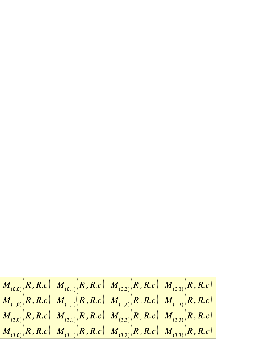
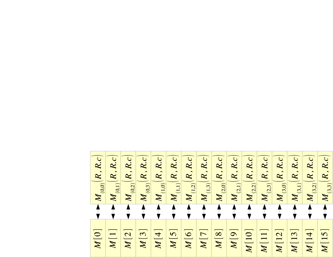
Figure 16: Top: It is conceptually easy to visualize the moments to be stored in a multi-dimensional array conceptually. Each dimension iterates over $p_{\mathit{max}}$ scalars, giving a total count of $\left(p_{\mathit{max}}\right)^{D}$ scalars. Bottom: The linear layout for the storing the coefficients.

Note that the FGT ensures: $\left|\widetilde{G}(q_{i},\mathcal{R})-G(q_{i},\mathcal{R})\right|\leq\tau$. Therefore, we first set $\tau=\epsilon$, halving $\tau$ until the error tolerance $\epsilon$ was met; the time for verifying the global error guarantee (which includes comparison against the naively computed results) was not included in the timing. For the FFT, we started with 16 grid points along each dimension, and doubled the number of grid points until the error guarantee was met. For the IFGT, we took the most recent version of the algorithm that does automatic parameter tuning described in [13]. Our algorithms based on dual-tree methods guarantees the error bound automatically via a direct parameter $\epsilon$.

The naive timings for the last datasets have been extrapolated from the performances on the smaller datasets. Our results demonstrate that our new algorithm can be as 15 times as fast as the original dual-tree algorithm. As expected, the grid-based original fast Gauss transform and the fast Fourier transformed based method fails in dimensions above two.

5 Conclusion

In this paper, we combined the two methods: the dual-tree KDE [8] and the original fast Gauss transform [11] to form the hierarchical form of the fast Gauss transform, the Dual-tree Fast Gauss Transform. Our results demonstrate that the $O(p^{D})$ expansion helps reduce the computational time on datasets of dimensionality up to 5.

Appendix: Implementing the Gaussian Series-expansion

This section explains how to implement the series-expansion mechanisms in computer languages such as C/C++.  
Storing the far-field/local moments as a linear array. Although the moments are inherently multi-dimensional, we store all coefficients in a C-style one-dimensional array. Each query node stores $\left(p_{\mathit{max}}\right)^{D}$ local moment terms. Similarly, each reference node stores $\left(p_{\mathit{max}}\right)^{D}$ far-field moment terms. These are allocated as a linear array during the construction of the two trees, as shown in Figure 16 which implies a bijective mapping between $D$-digit radix-$p_{\mathit{max}}$ numbers and decimal numbers between 0 and $p_{\mathit{max}}^{D}$ - 1 inclusive.

Converting between a position and a multi-index in the linear array. Algorithm 16 shows the mapping from a position in the linear array of $\left(p_{\mathit{max}}\right)^{D}$ terms to its corresponding multi-index. The algorithm converts the given position (given in base 10) to a number in base $p$.

Algorithm 16 $\mbox{{PositionToMultiindex}}(i,p)$: Converts the position of a linear array of length $p^{D}$ to its multi-index.

  {$i$-th position maps to the multi-index $\alpha$.}

  $\alpha_{i=1,\cdots,D}\leftarrow 0$

  for $d=D$ to $d=1$ do

     $\alpha[d-(D-1)]\leftarrow\left\lfloor\frac{i}{p}\right\rfloor$

     $i\leftarrow i\mod p$

  return  $\alpha$

Algorithm 17 converts the given multi-index to its corresponding position in the linear array of length $\left(p_{\mathit{max}}\right)^{D}$. It is basically an algorithm to convert a radix-$p_{\mathit{max}}$ number to its decimal representation.

Algorithm 17 $\mbox{{MultiIndexToPosition}}(\alpha)$: Converts the given multi-index to its corresponding position in the linear array of length $\left(p_{\mathit{max}}\right)^{D}$.

  {Converted position from the multi-index.}

  $x\leftarrow 0$,         $f\leftarrow 1$

  for $d=D$ to $d=1$ do

     $x\leftarrow x+f\cdot\alpha[d]$

     $f\leftarrow f\cdot p_{\mathit{max}}$

  return  $x$

Computing a multi-index expansion of a vector. A multi-index expansion of a vector $x\in\mathbb{R}^{D}$ up to $p^{D}$ terms is basically the set of coefficients $\{x^{\alpha}\}_{\alpha<p}$. See Figure 17. This is used in the process of forming a far-field moment contribution of a single reference point in AccumulateFarFieldMoment and evaluating a local expansion in EvalLocalExpansion.

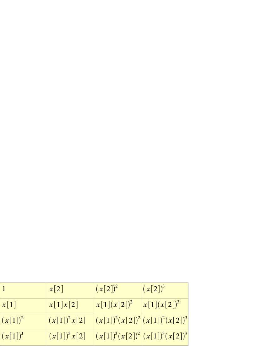
Figure 17: The multi-index expansion of a 2-D vector $x=[x[1],x[2]]^{T}$ up to 16 terms.

Algorithm 18 $\mbox{{MultiIndexExpansion}}(x,p,M^{\prime})$: Computes $M^{\prime}=\left\{x^{\alpha}\right\}_{\alpha<p}$.

  $M^{\prime}[0]\leftarrow 1$

  for each $i=0$ to $i=p^{D}-1$ do

     {Retrieve the multi-index mapping of the current position.}

     $\alpha\leftarrow\mbox{{PositionToMultiindex}}(i,p)$

     $j\leftarrow$ the first index of $\alpha$ such that $\alpha[j]\geq 1$.

     {Found a direct ancestor of the multiindex map $\alpha$.}

     $\alpha^{\prime}\leftarrow\alpha$,     $\alpha^{\prime}[j]\leftarrow\alpha^{\prime}[j]-1$

     {Recursively compute the $\alpha$-th multi-index component based on $\alpha^{\prime}$-th.}

     $M^{\prime}[i]\leftarrow M^{\prime}[\mbox{{MultiIndexToPosition}}(\alpha^{\prime})]\cdot x[j]$

Implementing the far-field moment accumulation (Equation (20)). This is straightforward given the implementation of the function
MultiIndexExpansion. Basically, it computes the multi-index of each reference point in the given reference node and accumulates each contribution and normalizes the sum. See Algorithm 19.

Algorithm 19 $\mbox{{AccumulateFarFieldMoment}}(R)$: Implements Equation (20).

  {Temporary space that is equal in size to $\{M_{\alpha}(R,R.c)\}_{\alpha<p_{\mathit{max}}}$.}

  $M^{\prime}_{i=0,\cdots,\left(p_{\mathit{max}}\right)^{D}-1}\leftarrow 0$

  for each $r_{j_{n}}\in R$ do

     {Add $M^{\prime}=\left\{\left(\frac{r_{j_{n}}-R.c}{\sqrt{2h^{2}}}\right)^{\alpha}\right\}_{\alpha<p_{\mathit{max}}}$ onto $\{M_{\alpha}(R,R.c)\}_{\alpha<p_{\mathit{max}}}$.}

     $\mbox{{MultiIndexExpansion}}\left(\frac{r_{j_{n}}-R.c}{\sqrt{2h^{2}}},p_{\mathit{max}},M^{\prime}\right)$

     $\{M_{\alpha}(R,R.c)\}_{\alpha<p_{\mathit{max}}}\leftarrow\{M_{\alpha}(R,R.c)\}_{\alpha<p_{\mathit{max}}}+M^{\prime}$

  for $i=0$ to $i=\left(p_{\mathit{max}}\right)^{D}-1$ do

     $M_{\alpha}(R,R.c)\leftarrow M_{\alpha}(R,R.c)\cdot\frac{1}{\alpha!}$

Implementing the far-to-far translation operator (shown in Algorithm 20). This consists of a doubly-nested for-loop over accumulated far-field moments.

Algorithm 20 $\mbox{{TransFarToFar}}(R^{\prime},R)$: Implements Equation (26).

  {Allocate space for and compute $\left\{\left(\frac{R^{\prime}.c-R.c}{\sqrt{2h^{2}}}\right)^{\alpha}\right\}_{\alpha<p_{\mathit{max}}}$.}

  $C_{i=0,\cdots,\left(p_{\mathit{max}}\right)^{D}-1}\leftarrow 0$

  $\mbox{{MultiIndexExpansion}}\left(\frac{R^{\prime}.c-R.c}{\sqrt{2h^{2}}},p_{\mathit{max}},C\right)$

  

  for $i=0$ to $i<(p_{\mathit{max}})^{D}$ do

     $\gamma\leftarrow\mbox{{PositionToMultiindex}}(i,p_{\mathit{max}})$

     for $j=0$ to $j<(p_{\mathit{max}})^{D}$ do

        $\alpha\leftarrow\mbox{{PositionToMultiindex}}(j,p_{\mathit{max}})$

        if $\alpha\leq\gamma$ then

           $M_{\gamma}(R,R.c)\leftarrow M_{\gamma}(R,R.c)+$

                    $\frac{1}{(\gamma-\alpha)!}M_{\alpha}(R^{\prime},R^{\prime}.c)\ \ \cdot\ \ C[\mbox{{MultiIndexToPosition}}(\gamma-\alpha)]$

Computing the multivariate Hermite functions. We exploit the fact that the multivariate Hermite functions is a product of $D$ univariate Hermite functions. Algorithm 21 computes partial derivatives of the Gaussian kernel evaluated at the given point $x$ along each dimension up to $p$-th order. $h_{\alpha}(x)=\prod\limits_{d=1}^{D}h_{\alpha[d]}(x)$ is a simple product of the univariate functions (see Algorithm 22).

Algorithm 21 $\mbox{{ComputePartialDerivatives}}(a,p,H)$: Evaluates the partial derivatives of $e^{-x^{2}/(2h^{2})}$ up to $(p-1)$-th order at each coordinate of $a$.

  for $d=1$ to $D$ do

     $H[d][0]\leftarrow e^{-(a[d])^{2}}$

     if $p>1$ then

        $H[d][1]\leftarrow 2\cdot a[d]\cdot e^{-(a[d])^{2}}$

        if $p>2$ then

           for $k=1$ to $k=p-2$ do

              $H[d][k+1]\leftarrow 2\cdot a[d]\cdot H[d][k]-2\cdot k\cdot H[d][k-1]$

Algorithm 22 $\mbox{{ComputeHermiteFunction}}(H,\alpha)$: Computes the Hermite function $h_{\alpha}(\cdot)$ using the pre-computed partial derivatives $H$.

  $f\leftarrow 1$

  for $d=1$ to $D$ do

     $f\leftarrow f\cdot H[d][\alpha[d]]$

  return  $f$

Evaluating a far-field expansion. Once the functions for computing the Hermite functions (Algorithm 21 and Algorithm 22), we can implement the function for evaluating a far-field expansion up to $p^{D}$ terms, as shown in Algorithm 23. The basic structure is one outer-loop over each query point and the inner loop iterating over each far-field moment. The contribution to each query point is computed as a dot-product between the far-field moment and the computed Hermite functions (see Figure 5).

Algorithm 23 $\mbox{{EvalFarFieldExpansion}}(R,Q,p)$: Evaluates the far-field expansion of the given reference node $R$ up to $p^{D}$ terms.

  {Allocate space for holding the partial derivatives.}

  $H_{\begin{subarray}{c}d=1,\cdots,D\\ k=0,\cdots,p-1\end{subarray}}\leftarrow 0$

  

  for each $q_{i_{m}}\in Q$ do

     {Compute partial derivatives up to $(p-1)$-th order along each dimension.}

     $\mbox{{ComputePartialDerivatives}}\left(\frac{q_{i_{m}}-R.c}{\sqrt{2h^{2}}},p,H\right)$

     $w\leftarrow 0$

     for $i=0$ to $i=p^{D}-1$ do

        $\alpha\leftarrow\mbox{{PositionToMultiindex}}(i,p)$

        $f\leftarrow\mbox{{ComputeHermiteFunction}}(H,\alpha)$

        $w\leftarrow w+M_{\alpha}(R,R.c)\cdot f$

     $\widetilde{G}(q_{i_{m}},\mathcal{R_{F}}(q_{i_{m}}))\leftarrow\widetilde{G}(q_{i_{m}},\mathcal{R_{F}}(q_{i_{m}}))+w$

Implementing the far-to-local translation operator. The basic structure of the algorithm is a doubly nested for-loop, each over the coefficients. The doubly-nested for-loop first translate a portion of the accumulated far-field moments of $R$ up to $p^{D}$ terms into the local moments. The final step of the algorithm is to add the translated moments $\{L_{\beta}(\{(R,T(Q.c,p))\})\}$ to the local moments stored in $Q$, $L_{\beta}(Q.c,\mathcal{R_{D}}(Q)\cup\mathcal{R_{T}}(Q))$. See Algorithm 24.

Algorithm 24 $\mbox{{TransFarToLocal}}(R,Q,p)$: Implements Equation (22).

  $H_{\begin{subarray}{c}d=1,\cdots,D\\ k=0,\cdots,2(p-1)\end{subarray}}\leftarrow 0$

  $\mbox{{ComputePartialDerivatives}}\left(\frac{Q.c-R.c}{\sqrt{2h^{2}}},2p-1,H\right)$

  

  for $i=0$ to $i=p^{D}-1$ do

     $\beta\leftarrow\mbox{{PositionToMultiindex}}(i,p)$

     for $j=0$ to $j=p^{D}-1$ do

        $\alpha\leftarrow\mbox{{PositionToMultiindex}}(j,p)$

        $f\leftarrow\mbox{{ComputeHermiteFunction}}(H,\alpha+\beta)$

        $L_{\beta}(\{(R,T(Q.c,p))\})\leftarrow L_{\beta}(\{(R,T(Q.c,p))\})+M_{\alpha}(R,R.c)\cdot f$

     $L_{\beta}(\{(R,T(Q.c,p))\})\leftarrow\frac{(-1)^{|\beta|}}{\beta!}L_{\beta}(\{(R,T(Q.c,p))\})$

  $\{L_{\beta}(Q.c,\mathcal{R_{D}}(Q)\cup\mathcal{R_{T}}(Q))\}_{\beta<p}\leftarrow\{L_{\beta}(Q.c,\mathcal{R_{D}}(Q)\cup\mathcal{R_{T}}(Q))\}_{\beta<p}+\left\{L_{\beta}(\{(R,T(Q.c,p))\})\right\}_{\beta<p}$

Implementing the direct local accumulation operation. The basic structure is a doubly-nested for-loop, the outer-loop over the reference points whose moments are to be accumulated as local moments and the inner loop over the coefficient positions. See Algorithm 25.

Algorithm 25 $\mbox{{AccumulateDirectLocalMoment}}(R,Q,p)$: Implements Equation (21).

  $H_{\begin{subarray}{c}d=1,\cdots,D\\ k=0,\cdots,p-1\end{subarray}}\leftarrow 0$,           $\{L_{\beta}(\{(R,D(Q.c,p))\})\}_{\beta<p}\leftarrow 0$

  for each $r_{j_{n}}\in R$ do

     $\mbox{{ComputePartialDerivatives}}\left(\frac{Q.c-r_{j_{n}}}{\sqrt{2h^{2}}},p,H\right)$

     for $i=0$ to $p^{D}-1$ do

        $\alpha\leftarrow\mbox{{PositionToMultiindex}}(i,p)$

        $f\leftarrow\textsc{ComputeHermiteFunction}(H,\beta)$

        $L_{\beta}(\{(R,D(Q.c,p))\})\leftarrow L_{\beta}(\{(R,D(Q.c,p))\})+f$

  $\{L_{\beta}(\{(R,D(Q.c,p))\})\}_{\beta<p}\leftarrow\{L_{\beta}(\{(R,D(Q.c,p))\})\}_{\beta<p}*\frac{(-1)^{|\beta|}}{\beta!}$

  $\{L_{\beta}(Q.c,\mathcal{R_{D}}(Q)\cup\mathcal{R_{T}}(Q))\}_{\beta<p}\leftarrow\{L_{\beta}(Q.c,\mathcal{R_{D}}(Q)\cup\mathcal{R_{T}}(Q))\}_{\beta<p}+\left\{L_{\beta}(\{(R,D(Q.c,p))\})\right\}_{\beta<p}$

Implementing the local-to-local translation operator. We direct readers’ attention to the first step of the algorithm, which retrieves the maximum order among used in local moment accumulation/translation. Then the algorithm proceeds with a doubly-nested for-loop over the local moments applies Equation (27). See Algorithm 26.

Algorithm 26 $\mbox{{TransLocalToLocal}}(Q^{\prime},Q)$: Implements Equation (27).

  {$p$ is the maximum approximation order used among the reference nodes pruned via far-to-local and direct local accumulations for $Q^{\prime}$.}

  $p\leftarrow\max\left\{\max\limits_{R\in\mathcal{R_{D}}(Q^{\prime})}p_{D},\max\limits_{R\in\mathcal{R_{T}}(Q^{\prime})}p_{T}\right\}$

  {Temporary space that is equal in size to $\{L_{\beta}\}$.}

  $X\leftarrow 0$

  $\mbox{{MultiIndexExpansion}}\left(\frac{Q.c-Q^{\prime}.c}{\sqrt{2h^{2}}},p,X\right)$

  for $j=0$ to $p^{D}-1$ do

     $\alpha\leftarrow\mbox{{PositionToMultiindex}}(j,p)$

     for $k=0$ to $p^{D}-1$ do

        $\beta\leftarrow\mbox{{PositionToMultiindex}}(k,p)$

        if $\beta\geq\alpha$ then

           $L_{\beta}(Q.c,\mathcal{R_{D}}(Q^{\prime})\cup\mathcal{R_{T}}(Q^{\prime}))\leftarrow L_{\beta}(Q.c,\mathcal{R_{D}}(Q^{\prime})\cup\mathcal{R_{T}}(Q^{\prime}))+$

                 $\frac{\beta!}{\alpha!(\beta-\alpha)!}L_{\beta}(Q^{\prime}.c,\mathcal{R_{D}}(Q^{\prime})\cup\mathcal{R_{T}}(Q^{\prime}))X_{\beta-\alpha}$

  $\{L_{\beta}(Q.c,\mathcal{R_{D}}(Q)\cup\mathcal{R_{T}}(Q))\}_{\beta<p}\leftarrow\{L_{\beta}(Q.c,\mathcal{R_{D}}(Q)\cup\mathcal{R_{T}}(Q))\}_{\beta<p}+\{L_{\beta}(Q.c,\mathcal{R_{D}}(Q^{\prime})\cup\mathcal{R_{T}}(Q^{\prime}))\}_{\beta<p}$

Evaluating the local expansion of the given query node. This function (see Algorithm 27) is consisted of one outer-loop over reference points and the inner-loop over the local moments up to $p^{D}$ terms, where $p$ is the maximum approximation order used among the reference nodes pruned via far-to-local and direct local accumulations for $Q$.

Algorithm 27 $\mbox{{EvalLocalExpansion}}(Q)$: Evaluates the accumulated local expansion of the given query node $Q$.

  {$p$ is the maximum approximation order used among the reference nodes pruned via far-to-local and direct local accumulations for $Q$.}

  $p\leftarrow\max\left\{\max\limits_{R\in\mathcal{R_{D}}(Q)}p_{D},\max\limits_{R\in\mathcal{R_{T}}(Q)}p_{T}\right\}$

  {Temporary space to hold the multi-index expansion of each $\left(\frac{q_{i_{m}}-Q.c}{\sqrt{2h^{2}}}\right)^{\alpha}$.}

  $X_{i=0,\cdots,p^{D}-1}\leftarrow 0$

  

  for each $q_{i_{m}}\in Q$ do

     $z\leftarrow 0$

     {Compute the multi-index expansion of $\frac{q_{i_{m}}-Q.c}{\sqrt{2h^{2}}}$ up to $p^{D}$ terms.}

     $\mbox{{MultiIndexExpansion}}\left(\frac{q_{i_{m}}-Q.c}{\sqrt{2h^{2}}},p,X\right)$

     for $i=0$ to $i=p^{D}-1$ do

        $\beta\leftarrow\mbox{{PositionToMultiindex}}(i,p)$

        $z\leftarrow z+L_{\beta}(Q.c,\mathcal{R_{D}}(Q)\cup\mathcal{R_{T}}(Q))\cdot z$

     $\widetilde{G}(q_{i_{m}},\mathcal{R_{D}}(q_{i_{m}})\cup\mathcal{R_{T}}(q_{i_{m}}))\leftarrow\widetilde{G}(q_{i_{m}},\mathcal{R_{D}}(q_{i_{m}})\cup\mathcal{R_{T}}(q_{i_{m}}))+z$

References

- [1] A. Appel. An efficient program for many-body simulation. SIAM Journal on Scientific and Statistical Computing, 6:85, 1985.
- [2] J. Barnes and P. Hut. A Hierarchical Force-Calculation Algorithm. Nature, 324, 1986.
- [3] B. Baxter and G. Roussos. A new error estimate of the fast Gauss transform. SIAM Journal on Scientific Computing, 24:257, 2002.
- [4] J. L. Bentley. Multidimensional Binary Search Trees used for Associative Searching. Communications of the ACM, 18:509–517, 1975.
- [5] P. B. Callahan. Dealing with Higher Dimensions: The Well-Separated Pair Decomposition and its Applications. PhD thesis, Johns Hopkins University, Baltimore, Maryland, 1995.
- [6] A. Gray and A. Moore. Rapid evaluation of multiple density models. Artificial Intelligence and Statistics, 2003.
- [7] A. Gray and A. Moore. Very fast multivariate kernel density estimation via computational geometry. In Joint Stat. Meeting, 2003.
- [8] A. Gray and A. W. Moore. N-Body Problems in Statistical Learning. In T. K. Leen, T. G. Dietterich, and V. Tresp, editors, Advances in Neural Information Processing Systems 13 (December 2000). MIT Press, 2001.
- [9] A. G. Gray and A. W. Moore. Nonparametric Density Estimation: Toward Computational Tractability. In SIAM International Conference on Data Mining 2003, 2003.
- [10] L. Greengard and V. Rokhlin. A Fast Algorithm for Particle Simulations. Journal of Computational Physics, 73, 1987.
- [11] L. Greengard and J. Strain. The Fast Gauss Transform. SIAM Journal of Scientific and Statistical Computing, 12(1):79–94, 1991.
- [12] D. Lee, A. Gray, and A. Moore. Dual-tree fast gauss transforms. In Y. Weiss, B. Schölkopf, and J. Platt, editors, Advances in Neural Information Processing Systems 18, pages 747–754. MIT Press, Cambridge, MA, 2006.
- [13] V. C. Raykar, C. Yang, R. Duraiswami, and N. Gumerov. Fast computation of sums of gaussians in high dimensions. Technical Report CS-TR-4767, Department of Computer Science, University of Maryland, CollegePark, 2005.
- [14] B. Silverman. Kernel Density Estimation using the Fast Fourier Transform. Journal of the Royal Statistical Society Series C: Applied Statistics, 33, 1982.
- [15] B. W. Silverman. Density Estimation for Statistics and Data Analysis. Chapman and Hall/CRC, 1986.
- [16] J. Strain. The fast Gauss transform with variable scales. SIAM Journal on Scientific and Statistical Computing, 12(5):1131–1139, 1991.
- [17] O. Szász. On the relative extrema of the hermite orthogonal functions. J. Indian Math. Soc., 15:129–134, 1951.
- [18] M. P. Wand. Fast Computation of Multivariate Kernel Estimators. Journal of Computational and Graphical Statistics, 1994.
- [19] C. Yang, R. Duraiswami, N. A. Gumerov, and L. Davis. Improved fast gauss transform and efficient kernel density estimation. International Conference on Computer Vision, 2003.