RELATIONAL QUADRILATERALLAND INTERPRETATION

OF $\mathbb{CP}^{2}$ AND QUOTIENTS

Edward Anderson¹

¹ Astroparticule et Cosmologie, Université Paris 7 Diderot

I investigate qualitatively significant regions of the configuration space for the classical and quantum mechanics of the relational quadrilateral in 2-d. This is relational in the sense that only relative ratios of separations, relative angles and relative times are significant. Such relational particle mechanics models have many analogies with the geometrodynamical formulation of general relativity. Thus, they are suitable as toy models for studying 1) problem of time in quantum gravity strategies, in particular timeless, semiclassical and histories theory approaches and combinations of these. 2) Various other quantum-cosmological issues, such as structure formation/inhomogeneity and the significance of uniform states. The relational quadrilateral is more useful in these respects than previously investigated simpler RPM’s as it possesses linear constraints, nontrivial subsystems and its configuration space is a nontrivial complex-projective space. In this paper, I investigate the submanifold of collinear configurations, the submanifolds with a single-particle collision, the square configurations and regions of the configuration space for which such as approximate collinearity, approximate squareness and approximate triangularity hold. I consider both mirror image identified and unidentified shapes, as well as both distinguishable and indistinguishable particle labels. I find the following $\mathbb{CP}^{2}$ coordinate systems to be useful for these purposes. 1) Kuiper’s coordinates, which, for quadrilateralland, are magnitudes of the Jacobi vectors and anisoscelesnesses of the triangles formed between them. 2) Gibbons–Pope type coordinates, which, for quadrilateralland, are the sum and difference of relative angles between subsystems, the ratio of size of 2 subsystems and the proportion of universe model occupied by the subsystems.

Seminar II on relational quadrilaterals

PACS: 04.60Kz.

¹ edward.anderson@apc.univ-paris7.fr (Work started at DAMTP Cambridge and continued at UAM Madrid)

1 Introduction

Relational particle mechanics (RPM) are mechanics in which only relative times, relative angles and (ratios of) relative separations are physically meaningful. Scaled RPM was set up in [2] by Barbour and Bertotti and pure-shape (i.e. scalefree, and so involving just ratios) RPM was set up in and in [3] by Barbour. These theories are relational in Barbour’s sense as opposed to Rovelli’s [4, 5, 6, 7, 43], via obeying the following postulates.

1) RPM’s are temporally relational [2, 8, 9]. I.e. they do not possess any meaningful primary notion of time for the whole (model) universe. This is implemented by using actions that are manifestly reparametrization invariant while also being free of extraneous time-related variables [such as Newtonian time or the lapse in General Relativity (GR)]. These actions are of the form

$$\mbox{I}=2\int\textrm{d}s\sqrt{\mbox{E}-\mbox{V}}\mbox{ }.$$ (1)

(Jacobi-type actions [10] for mechanics, which are closely related to Baierlein–Sharp–Wheeler-type actions [11, 8] for GR in geometrodynamical form.) This reparametrization invariance then directly produces primary constraints quadratic in the momenta. In the GR case, the constraint arising thus is the super-Hamiltonian constraint,

$${\cal H}:=N_{ijkl}\pi^{ij}\pi^{kl}/\sqrt{h}-\sqrt{h}\{R-2\Lambda\}=0\mbox{ },$$ (2)

whilst for RPM’s it gives an energy constraint,

$$\mbox{\tt H}:=\sum\mbox{}_{\mbox{}_{\mbox{\scriptsize$e$ = 1}}}^{n}P_{e}\mbox{}^{2}/2\mu_{e}+\mbox{V}=\mbox{E}\mbox{ }.$$ (3)

2) RPM’s are configurationally relational. This can be thought of as some group $G$ of transformations that act on the theory’s configuration space $Q$ being taken to be physically meaningless [2, 8, 9, 12, 13]. Configurational relationalism can be approached by [2, 3] indirect means that amount to working on the principal bundle P($Q$, $G$). In this setting, linear constraints arise from varying with respect to the $G$-generators. In the case of GR, such a variation with respect to the generators of the 3-diffeomorphisms gives the super-momentum constraint

$${\cal L}_{i}:=-2D_{j}{\pi^{j}}_{i}=0\mbox{ },$$ (4)

whilst for RPM’s variation with respect to the generators of the rotations gives that the total angular momentum for the model universe as a whole is constrained to be zero,

$${\bf L}:=\sum\mbox{}_{\mbox{}_{\mbox{\scriptsize$e$ = 1}}}^{n}{\bf R}^{e}\mbox{\scriptsize{\bf$\mbox{ }\times\mbox{ }$}}{\mbox{\bf P}}_{e}=0\mbox{ }.$$ (5)

In the case of pure-shape RPM, variation with respect to the generator of the dilations gives that the total dilational momentum of the model universe is constrained to be zero,

$$\mbox{\tt D}:=\sum\mbox{}_{\mbox{}_{\mbox{\scriptsize$e$ = 1}}}^{n}{\bf R}^{e}\cdot{\mbox{\bf P}}_{e}=0\mbox{ }.$$ (6)

Next, elimination of the $G$-generator variables from the Lagrangian form of these constraints sends one to the desired quotient space $Q/G$. In 1- and 2-$d$, these RPM’s can be obtained alternatively by working directly on $Q/G$ [9, 13] (see Sec 3 to 5 for further details). This involves applying a ‘Jacobi–Synge’ construction of the natural mechanics associated with a geometry, to Kendall’s shape spaces [14] for pure-shape RPM’s or to the cones over these [13] for the scaled RPM’s.

RPM’s are further motivated as useful toy models [15, 5, 8, 16, 17, 18, 19, 20, 12, 21, 13] of yet further features of GR cast in geometrodynamical form. RPM’s are similar in complexity and in number of parallels with GR to minisuperspace [22] and to 2 + 1 GR [23] are, though each such model differs in how it resembles GR, so that such models offer complementary perspectives and insights. In particular

I) The analogies with GR continue at the level of configuration spaces (see Fig 2 in Sec 2).

II) RPM’s energy constraint parallels the GR super-Hamiltonian constraint ${\cal H}$ in leading to the frozen formalism facet of the Problem of Time. This notorious problem occurs because ‘time’ takes a different meaning in each of GR and ordinary quantum theory. This incompatibility underscores a number of problems with trying to replace these two branches with a single framework in situations in which the premises of both apply, such as in black holes or the very early universe. One facet of the Problem of Time that then appears in attempting canonical quantization of GR is due to ${\cal H}$ being quadratic but not linear in the momenta, which feature and consequence are shared by H. Then elevating ${\cal H}$ to a quantum equation produces a stationary i.e timeless or frozen wave equation: the Wheeler-DeWitt equation

$$\widehat{\cal H}\Psi=0\mbox{ },$$ (7)

instead of ordinary QM’s time-dependent one,

$$i\hbar\partial\Psi/\partial t=\widehat{H}\Psi$$ (8)

(where I use $\Psi$ for the wavefunction of the universe, $H$ to denote a Hamiltonian and $t$ for absolute Newtonian time). See [15, 24, 25] for other facets of the Problem of Time.

III) The nontrivial linear constraints parallel the GR momentum constraint (and are absent for minisuperspace), which is the cause of a number of further difficulties in various approaches to the Problem of Time.

By parallels I), II) and III), RPM s are appropriate as toy models for a large number of Problem of Time approaches [see the Conclusion for more details]. Other useful applications of RPM’s not covered by minisuperspace models include

IV) that RPM’s are useful for the qualitative study of the quantum-cosmological origin of structure formation/ inhomogeneity. (Scaled RPM’s are a tightly analogous, simpler version of Halliwell and Hawking’s [26] model for this; moreover scalefree RPM’s such as this paper’s occurs as a subproblem within scaled RPM’s, corresponding to the light fast modes/inhomogeneities.)

V) RPM’s are likewise useful for the study of correlations between localized subsystems of a given instant.

VI) RPM’s also allow for a qualitative study of notions of uniformity/of maximally or highly uniform states in classical and quantum Cosmology, which are held to be conceptually important notions in these subjects.

Some of the analogies with GR already hold for the 1-d $N$-stop metroland RPM’s, which have the particularly tractable {$N$ – 2}-spheres $\mathbb{S}^{N-2}$ as shape spaces. 2-$d$ suffices for almost all the analogies with GR to hold whilst still keeping the mathematics manageable; the shape spaces are the complex projective spaces $\mathbb{CP}^{N-2}$. $N$-stop metroland and triangleland RPM’s have already been covered in [21, 18, 7, 27, 28, 29]. Thus, we are now looking at the next $N$-a-gonland: the $N$ = 4 case, quadrilateralland. This is valuable through its simultaneously possessing the following features.

1) Nontrivial linear constraints.

2) Nontrivial clustering/inhomogeneity/structure (i.e. midisuperspace-like features rendering it suitable as a qualitative toy model of Halliwell and Hawking’s quantum cosmological origin of structure formation in the universe).

3) Relationally nontrivial non-overlapping subsystems and hierarchies of nontrivial subsystems. [These are useful features for timeless approaches as well as for a less trivial structure formation than in the triangleland case.]

Also, quadrilateralland possesses nontrivial complex projective space mathematics (triangleland atypically simplifies via $\mathbb{CP}^{1}=\mathbb{S}^{2}$, whereas quadrilateralland is much more mathematically typical for an $N$-a-gonland.)

I emphasize that the study of quadrilateralland is still at an early stage. In a previous paper [30], I considered i) shape quantities for quadrilateralland that parallel the Dragt-type coordinates [31] that were so useful for triangleland [28, 29] (and are closely related to the Hopf map). ii) The clustering-independent (‘democratically invariant’ [32, 33]) properties for this. iii) This leads to a quantifier of uniformity for model-universe configurations. The present paper is the first instance in RPM literature involving detailed treatment of indistinguishable particles as well as the first paper on submanifolds within $\mathbb{CP}^{2}$ interpreted in quadrilateralland terms. These two papers, and a third concerning the interpretation of $\mathbb{CP}^{2}$’s $SU(3)$ of conserved quantities in quadrilateralland terms [34], are important prerequisites for the subsequent study of the classical and quantum mechanics of quadrilateralland [35]. These are then useful as a nontrivial model of the Problem of Time in Quantum Gravity and of various other foundational and qualitative issues in Quantum Cosmology (extending e.g. [29, 49, 43]).

A distinct physical interpretation of $\mathbb{CP}^{2}$ is as qtrits in Quantum Information Theory. qtrits and q$n$its in general are motivated by there being much more information storage in these than in qbits. $\mathbb{CP}^{N-2}$ occurs in this application as the space of quantum states. Thus additionally qtrits can also be interpreted in terms of quadrilaterals and qu$n$its in terms of $N$-a-gons for $N=n+1$.

For more uses of $\mathbb{CP}^{2}$, see [58, 34].

In Sec 2 I provide coordinate systems and types of configuration space that are useful in the study of the general relational particle mechanics models. I then consider details of the configuration spaces for 4-stop metroland (Sec 3) and triangleland (Sec 4), alongside further coordinatizations useful in these specific cases. These (and extensions of them) then feature within the paper’s main focus, quadrilateralland (Sec 5). For $\mathbb{CP}^{2}$, a useful set of redundant coordinates are Kuiper coordinates [36]. These are interpretable in the quadrilateralland setting as magnitudes of the Jacobi vectors alongside the inner products between pairs of these. The latter amount to relative angles, interpretable as the departures from isoscelesness of the coarse-graining triangles associated with the quadrilateral (or departure from rhombicness of the coarse-graining parallelogram). I use these to determine the quadrilateralland counterpart of the split of triangleland’s sphere into two hemispheres of mirror-image configurations that join along an equator of collinear configurations (which is one of [28]’s most important and useful results). Another useful set of coordinates for $\mathbb{CP}^{2}$ are Gibbons–Pope type coordinates [37] (intrinsic to $\mathbb{CP}^{2}$ itself). In this paper I interpret these in quadrilateralland terms, showing how spherical coordinates for both 4-stop metroland and triangleland extend neatly into this this set of quadrilateralland coordinates. These give a clear way of seeing how the $\mathbb{CP}^{2}$ metric reduces to a $\mathbb{S}^{2}$ one when two of the particles collide so that one is left with a triangular configuration. I also investigate the square configurations and a weaker notion of highly uniform states using both of the above coordinate systems. In the conclusion (Sec 6), I include a further application of the Gibbons–Pope type coordinates to quadrilateralland: for computing integrals over geometrically/physically significant regions of the quadrilateralland shape space (these are relevant to various approaches to the Problem of Time) and comment on the $N$-a-gonland extension of the present paper.

2 Coordinate systems used in this paper

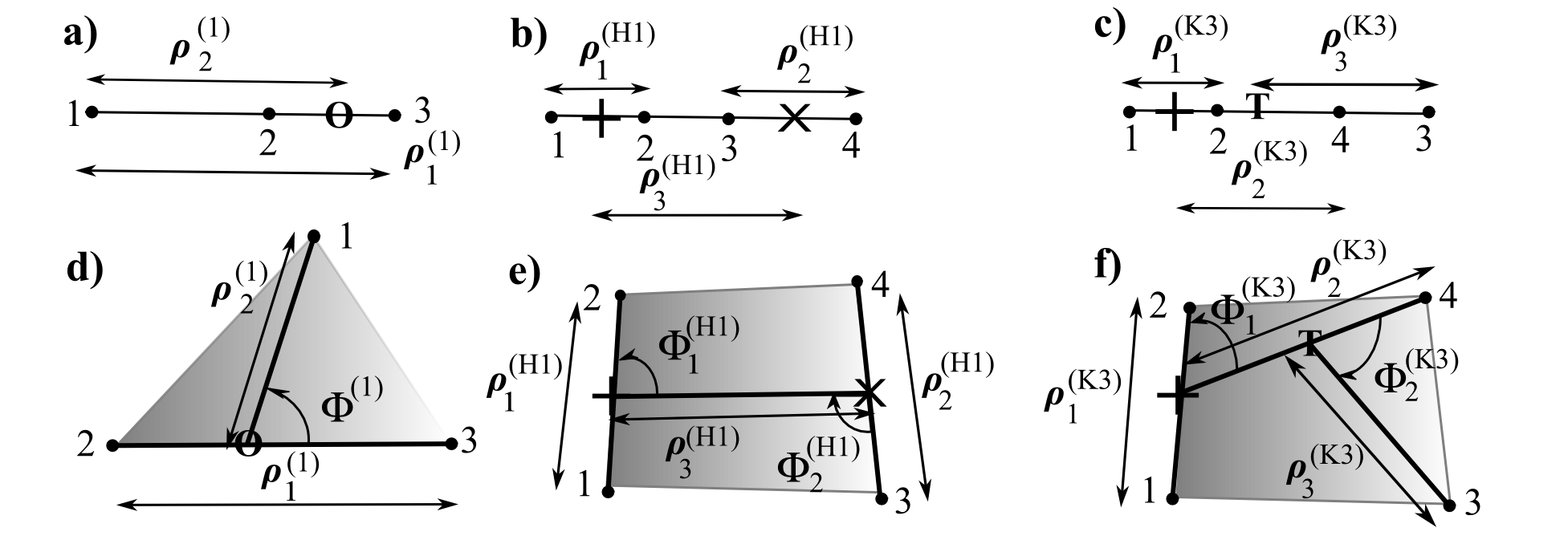
Figure 1: O, +, $\times$ and T denote COM(23), COM(12), COM(34) and COM(124) respectively, where COM(ab) is the centre of mass of particles a and b. a) For 3 particles in 1-$d$, one particular choice of mass-weighted relative Jacobi coordinates are as indicated. I use (Hb) as shorthand for {ab, cd} i.e. the clustering (partition into subclusters) into two pairs {ab} and {cd}, and (Ka) as shorthand for {{cd, b}, a} i.e. the clustering into a single particle a and a triple {cd, b} which is itself partitioned into a pair cd and a single particle b. In each case, a, b, c, d form a cycle. In this paper, I take clockwise and anticlockwise labelled triangles to be distinct, i.e. I make the plain rather than mirror-image-identified choice of set of shapes. I also assume equal masses for simplicity. For 4 particles in 1-$d$, b) and c) give, respectively, a particular choice of mass-weighted relative Jacobi H-coordinates [the squashed version of the obvious H-shape in e)] and of Jacobi K-coordinates [the squashed version of the obvious K-shape in f)]. This paper also represents a fair amount of RPM work done for the first time in Jacobi K-coordinates Later references to H and K coordinates refer explicitly to the (H1) and (K3) cases depicted above; I drop these labels to simplify the notation. d) For 3 particles in 2-$d$, one particular choice of mass-weighted relative Jacobi coordinates are as indicated. I furthermore define $\Phi^{(\mbox{\scriptsize a})}$ as the ‘Swiss army knife’ angle $\mbox{arccos}\big{(}\mbox{\boldmath$\rho$}_{1}^{(\mbox{\scriptsize a})}\cdot\mbox{\boldmath$\rho$}_{3}^{(\mbox{\scriptsize a})}/\rho_{1}^{(\mbox{\scriptsize a})}\rho_{3}^{(\mbox{\scriptsize a})}\big{)}$. For 4 particles in 2-$d$ e) and f) give, respectively, a particular choice of mass-weighted relative Jacobi H-coordinates [with $\Phi_{1}^{(\mbox{\scriptsize H}\mbox{\scriptsize b})}$ and $\Phi_{2}^{(\mbox{\scriptsize H}\mbox{\scriptsize b})}$ as the ‘Swiss army knife’ angles $\mbox{arccos}\big{(}\mbox{\boldmath$\rho$}_{1}^{(\mbox{\scriptsize H}\mbox{\scriptsize b})}\cdot\mbox{\boldmath$\rho$}_{3}^{(\mbox{\scriptsize H}\mbox{\scriptsize b})}/\rho_{1}^{(\mbox{\scriptsize H}\mbox{\scriptsize b})}\rho_{3}^{(\mbox{\scriptsize H}\mbox{\scriptsize b})}\big{)}$ and $\mbox{arccos}\big{(}\mbox{\boldmath$\rho$}_{2}^{(\mbox{\scriptsize H}\mbox{\scriptsize b})}\cdot\mbox{\boldmath$\rho$}_{3}^{(\mbox{\scriptsize H}\mbox{\scriptsize b})}/\rho_{2}^{(\mbox{\scriptsize H}\mbox{\scriptsize b})}\rho_{3}^{(\mbox{\scriptsize H}\mbox{\scriptsize b})}\big{)}$ respectively] and of K-coordinates [with $\Phi_{1}^{(\mbox{\scriptsize K}\mbox{\scriptsize a})}$ and $\Phi_{2}^{(\mbox{\scriptsize K}\mbox{\scriptsize a})}$ as the ‘Swiss army knife’ angles $\mbox{arccos}\big{(}\mbox{\boldmath$\rho$}_{1}^{(\mbox{\scriptsize K}\mbox{\scriptsize a})}\cdot\mbox{\boldmath$\rho$}_{2}^{(\mbox{\scriptsize K}\mbox{\scriptsize a})}/\rho_{1}^{(\mbox{\scriptsize K}\mbox{\scriptsize a})}\rho_{2}^{(\mbox{\scriptsize K}\mbox{\scriptsize a})}\big{)}$ and arccos$\big{(}\mbox{\boldmath$\rho$}_{2}^{(\mbox{\scriptsize K}\mbox{\scriptsize a})}\cdot\mbox{\boldmath$\rho$}_{3}^{(\mbox{\scriptsize K}\mbox{\scriptsize a})}/\rho_{2}^{(\mbox{\scriptsize K}\mbox{\scriptsize a})}\rho_{3}^{(\mbox{\scriptsize K}\mbox{\scriptsize a})}\big{)}$ respectively].

$N$ particles in dimension $d$ has Cartesian configuration space $\mathbb{R}^{dN}$. Rendering absolute position irrelevant (e.g. by passing from particle position coordinates ${\bf q}^{a}$ to any sort of relative coordinates) leaves one on the configuration space relative space, $\mbox{R}=\mathbb{R}^{2n}$, for $n$ = $N$ – 1. The most convenient sort of coordinates for this are relative Jacobi coordinates [38] ${\bf R}^{e}$. These are combinations of relative position vectors ${\bf r}^{ab}={\bf q}^{b}-{\bf q}^{a}$ between particles into inter-particle cluster vectors such that the kinetic term is diagonal. Relative Jacobi coordinates have associated particle cluster masses $\mu_{e}$. In fact, it is tidier to use mass-weighted relative Jacobi coordinates $\mbox{\boldmath$\rho$}^{e}=\sqrt{\mu_{e}}{\bf R}^{e}$ (Fig 1). The squares of the magnitudes of these are the partial moments of inertia $I^{e}=\mu_{e}|{\bf R}^{e}|^{2}$. I also denote $|\mbox{\boldmath$\rho$}^{e}|$ by $\rho^{e}$, $I^{e}/I$ by $N^{e}$ for $I$ the moment of inertia of the system, and $\mbox{\boldmath$\rho$}^{e}/\rho$ by $\mbox{\bf n}^{e}$ for $\rho=\sqrt{I}$ the hyperradius. If one quotients out the rotations also, one is on relational space ${\cal R}(N,d)$. If one furthermore quotients out the scalings, one is on shape space $\mbox{S}(N,d)$. If one quotients out the scalings but not the rotations, one is on preshape space [14] $\mbox{P}(N,d)$ [see Fig 2a)].

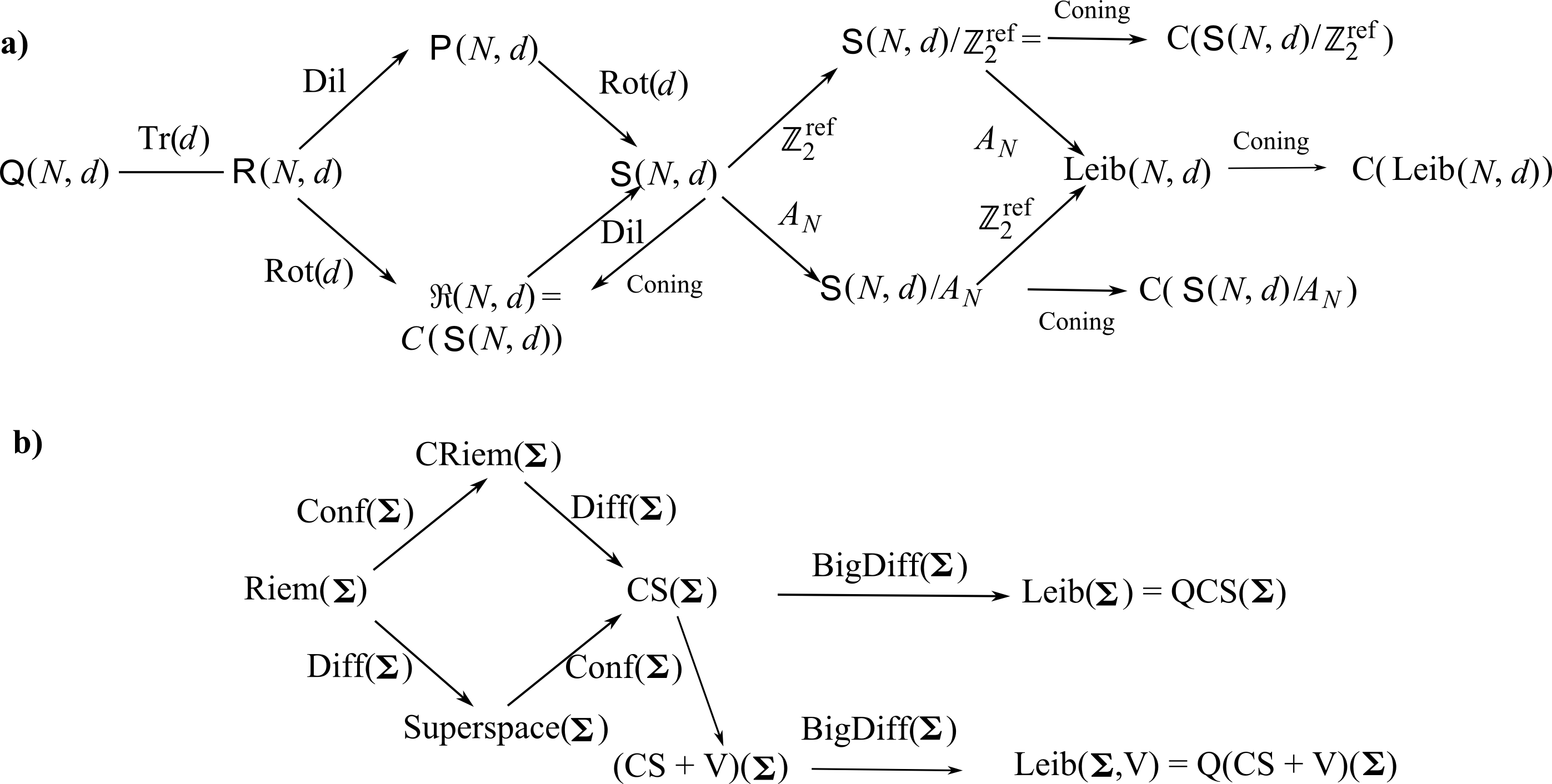
Figure 2: a) the sequence of configuration spaces of this paper. b) The corresponding sequence of configuration spaces for GR. Riem($\Sigma$) is the space of positive-definite 3 metrics on a fixed topology $\Sigma$, taken to be a compact without boundary one for simplicity. These most naturally correspond to relative space R($N,d$). Diff($\Sigma$) and Conf($\Sigma$) are the corresponding 3-diffeomorphisms and conformal transformations; these most naturally correspond to the rotations Rot($d$) and dilations Dil respectively. Superspace($\Sigma$) is Wheeler’s notion [39] (entirely unrelated to the later use of this word in the context of supersymmetry). CRiem($\Sigma$) is pointwise superspace and CS($\Sigma$) is conformal superspace. Superspace($\Sigma$), CRiem($\Sigma$) and CS($\Sigma$) most naturally correspond to relational space ${\cal R}(N,d)$, preshape space P($N,d$) and shape space S($N,d$) respectively. (RPM’s also admit analogies with conformal/York-type [40] initial value problem formulations of GR, with the conformal 3-geometries playing here an analogous role to the pure shapes.) (CS + V)($\Sigma$) is conformal superspace to which has been adjoined a single global degree of freedom: the spatial volume of the universe. CS($\Sigma$) and (CS + V)($\Sigma$) have on a number of occasions been claimed to be the space of true dynamical degrees of freedom of GR [40, 41]. The quotienting out of large diffeomorphisms gives the notion of quantum superspace and quantum conformal superspace [QCS($\Sigma$)] as per [42]. This corresponds most naturally to identifying mirror image shapes and enforcing particle indistinguishability. Leib($N,d)=\mbox{S}(N,d)/S_{N}$ is then the analogue of QCS($\Sigma$) and C(Leib($N,d$)) is then in some ways the analogue of quantum CS + V. It is named thus as the most very Leibnizian of the possible configuration spaces for mechanics with equal particle masses.

For $N$ particles in 1-$d$, preshape space is $\mathbb{S}^{N-2}$ (or some piece thereof, see Sec 3) which coincides with shape space. For $N$ particles in 2-$d$, preshape space is $\mathbb{S}^{nd-1}$ and shape space is $\mathbb{CP}^{N-2}$ (provided that the plain choice of set of shapes is made). The 3-particle case of this is, moreover, special, by $\mathbb{CP}^{1}=\mathbb{S}^{2}$. Also, relational space ${\cal R}(N,d)$ is equal to [13] the cone over shape space, denoted by $\mbox{C}(\mbox{S}(N,d))$. [At the topological level, for C(X) to be a cone over some topological manifold X,

$$\mbox{C(X) = X $\times$ [0, $\infty$)/\mbox{ }$\widetilde{\mbox{ }}$}\mbox{ },$$ (9)

where $\widetilde{\mbox{ }}$ means that all points of the form {p $\in$ X, 0 $\in[0,\infty)$} are ‘squashed’ or identified to a single point termed the cone point, and denoted by 0. For what a cone further signifies at the level of Riemannian geometry, see below.] In particular, ${\cal R}(N,1)=\mbox{C}(\mathbb{S}^{N-2})=\mathbb{R}^{n}$ and ${\cal R}(N,2)$ = C$(\mathbb{CP}^{N-2})$ [among which additionally $\mbox{C}(\mathbb{CP}^{1})=\mbox{C}(\mathbb{S}^{2})=\mathbb{R}^{3}$ at the topological level]. Thus, this paper’s quadrilateralland case is the first case with nontrivial complex-projective mathematics.

For 1-$d$, one has the usual {$N$ – 2}-sphere metric on shape space, $\textrm{d}^{2}s_{\mbox{\scriptsize s}\mbox{\scriptsize p}\mbox{\scriptsize h}\mbox{\scriptsize e}}$, with then the Euclidean metric on the corresponding relational space, $\textrm{d}^{2}s_{\mbox{\scriptsize E}\mbox{\scriptsize u}\mbox{\scriptsize c}\mbox{\scriptsize l}}=\textrm{d}\rho^{2}+\rho^{2}\textrm{d}^{2}s_{\mbox{\scriptsize s}\mbox{\scriptsize p}\mbox{\scriptsize h}\mbox{\scriptsize e}}$. For 2-$d$, the kinetic metric on shape space is the natural Fubini–Study metric [14, 9],

$$\textrm{d}s_{\mbox{\scriptsize F}\mbox{\scriptsize S}}^{2}=\big{\{}\{1+|{\mbox{Z}}|_{\mbox{\scriptsize c}}^{2}\}|\textrm{d}{\mbox{Z}}|_{\mbox{\scriptsize c}}^{2}-|({\mbox{Z}},\textrm{d}\overline{{\mbox{Z}}}\}_{\mbox{\scriptsize c}}|^{2}\big{\}}/\{1+|{\mbox{Z}}|_{\mbox{\scriptsize c}}^{2}\}^{2}\mbox{ }.$$ (10)

I explain the coordinates in use here as follows. Firstly, {${\mbox{z}}^{e}$} are, mathematically, complex homogeneous coordinates for $\mathbb{CP}^{2}$; I denote their polar form by $\mbox{z}^{e}=\rho^{e}\mbox{exp}({i\phi^{e}})$. Physically, these contain 2 redundancies and their moduli are the magnitudes of the Jacobi vectors whilst their arguments are angles between the Jacobi vectors and an absolute axis. Next, {${\mbox{Z}}^{I}$} are, mathematically, complex inhomogeneous coordinates for $\mathbb{CP}^{2}$; I denote their polar form by $\mbox{Z}^{I}={\cal R}^{I}\mbox{exp}({i\Phi^{I}})$. These are independent ratios of the $\mbox{z}^{e}$, and so, physically their magnitudes ${\cal R}^{I}$ are ratios of magnitudes of Jacobi vectors, and their arguments $\Phi^{I}$ are now angles between Jacobi vectors, which are entirely relational quantities. Also, I use $|{\mbox{Z}}|_{\mbox{\scriptsize c}}^{2}:=\sum_{I}|{\mbox{Z}}^{I}|^{2}$, $(\mbox{ },\mbox{ })_{\mbox{\scriptsize c}}$ for the corresponding inner product, overline to denote complex conjugate and $|\mbox{ }|$ to denote complex modulus. Note that using the polar form for the $\mbox{Z}^{I}$, the line element and the corresponding kinetic term can be cast in a real form. The kinetic metric on relational space in scale-shape split coordinates is then of the cone form

$$\textrm{d}s_{\mbox{\scriptsize C}(\mbox{\scriptsize F}\mbox{\scriptsize S})}^{2}=\textrm{d}\rho^{2}+\rho^{2}\textrm{d}s_{\mbox{\scriptsize F}\mbox{\scriptsize S}}^{2}\mbox{ }$$ (11)

[for $\textrm{d}s^{2}$ is the line element of X itself and $\rho$ a suitable ‘radial variable’ that parametrizes the [0, $\infty$), which is the distance from the cone point; such ‘cone metrics’ are smooth everywhere except (possibly) at the troublesome cone point].

The action for RPM’s in relational form is then (1), which is a Jacobi-type action [10] (thus complying with temporal relationalism), with, in 1- or 2-$d$, $\mbox{T}=\mbox{T}_{\mbox{\scriptsize s}\mbox{\scriptsize p}\mbox{\scriptsize h}\mbox{\scriptsize e}}$ or $\mbox{T}_{\mbox{\scriptsize E}\mbox{\scriptsize u}\mbox{\scriptsize c}\mbox{\scriptsize l}}$, $\mbox{T}=\mbox{T}_{\mbox{\scriptsize F}\mbox{\scriptsize S}}$ or $\mbox{T}_{\mbox{\scriptsize C}(\mbox{\scriptsize F}\mbox{\scriptsize S})}$ built from the above selection of metrics (thus directly implementing configurational relationalism).

3 4-stop metroland

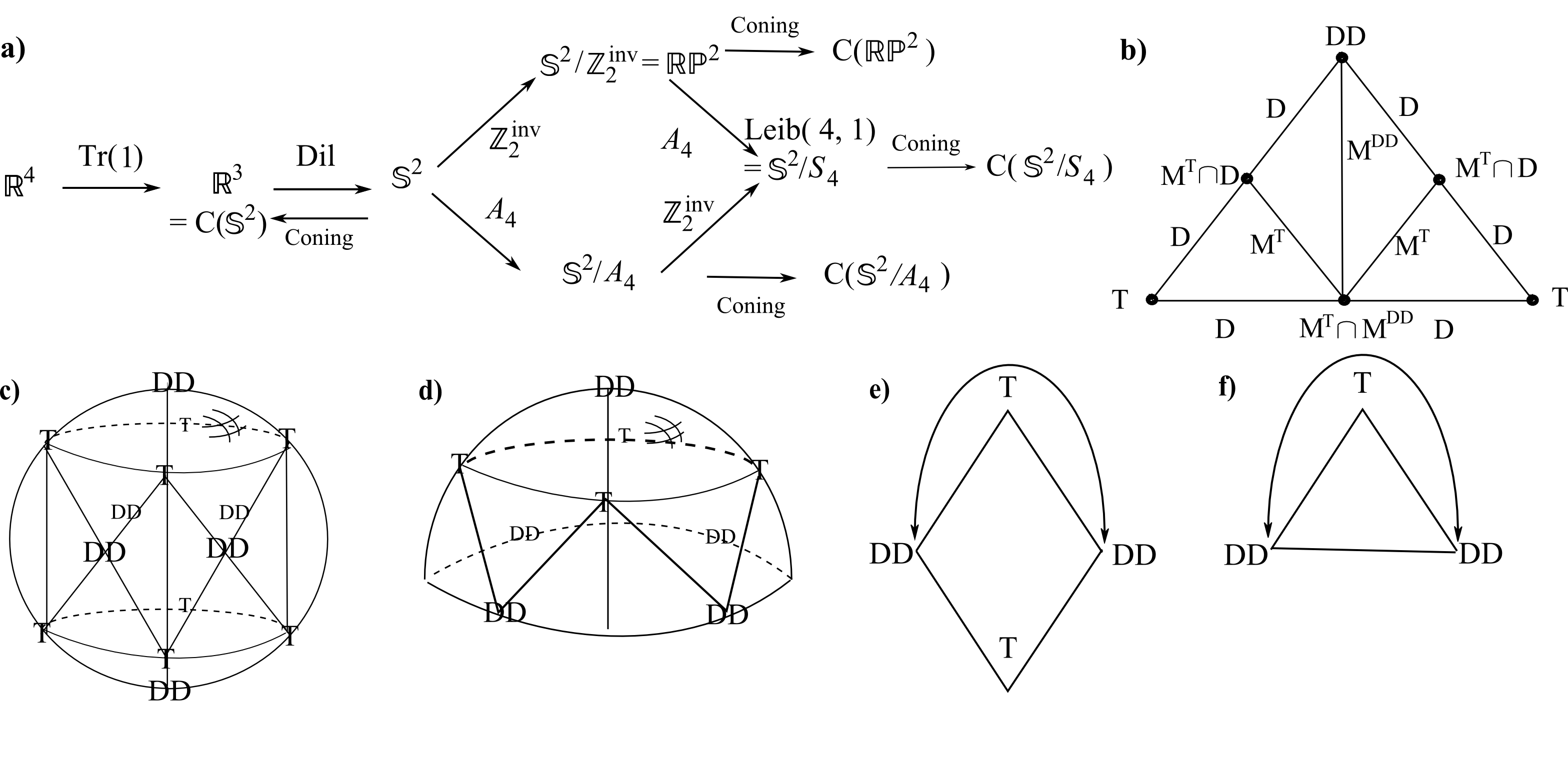
Figure 3: a) The sequence of configuration spaces for 4-stop metroland. c) and d) are the tessellations for the distinguishable particles plain shape and mirror image identified cases respectively. b) illustrates the notions of merger within a single triangular face. There are $\mbox{M}^{\mbox{\tiny T}}$ arcs (for which the fourth particle is at the centre of mass of the other three) and $\mbox{M}^{\mbox{\tiny D}\mbox{\tiny D}}$ arcs (for which the centre of mass of 2 pairs of particles coincide), as well as $\mbox{M}^{\mbox{\tiny T}}\bigcap\mbox{D}$ and $\mbox{M}^{\mbox{\tiny D}\mbox{\tiny D}}\bigcap\mbox{M}^{\mbox{\tiny T}}$ points. These are also the types of merger present in quadrilateralland. d) and e) are then the indistinguishable particle counterparts of these.

The configuration space here for distinguishable particles and in the plain shape case is the sphere, decorated with the physical interpretation of Figs 3c). All the lines in Fig 3c) to f) are lines of double collisions, D. The DD points are double double collisions (two separate double collisions) whilst the T points are triple collisions.

At the level of configuration space geometry, the mirror-image-identification in space becomes inversion about the centre of the sphere. This gives rise to the real projective space, $\mathbb{RP}^{2}$ [Fig 3c)]. Indistinguishability then involves quotienting out $S_{4}$ (permutations of the particles, which is isomorphic to the cube or octahaedron group acting on the DD’s or the T’s), as in Fig 3f). If there is no mirror-image identification, the quotienting out is rather by $A_{4}$ (even permutations of the particles, isomorphic to the group of the cube or the octahaedron excluding one reflection operation), as in Fig 3e).

For later comparison with quadrilateralland [with matching enumeration, hence the absense of 2) and 3) below],

1) A useful set of redundant coordinates for a surrounding flat Euclidean space (here equal to relational space) are, for 4-stop metroland, simply the three relative Jacobi coordinate magnitudes, $\mbox{n}^{e}$.

4) Useful coordinates intrinsic to the shape space itself are the spherical polar coordinates $\theta$ and $\phi$, which have the following 4-stop metroland interpretations. In Jacobi H-coordinates,

$$\theta=\mbox{arctan}\big{(}\sqrt{\rho_{1}\mbox{}^{2}+\rho_{2}\mbox{}^{2}}/\rho_{3}\big{)}\mbox{ },\mbox{ }\mbox{ }\phi=\mbox{arctan}(\rho_{2}/\rho_{1})\mbox{ },$$ (12)

which are respectively a measure of the size of the universe’s contents relative to the size of the whole model universe, and a measure of inhomogeneity among the contents of the universe (whether one of the constituent clusters is larger than the other one.) On the other hand, for Jacobi K-coordinates

$$\theta=\mbox{arctan}\big{(}\sqrt{\rho_{1}\mbox{}^{2}+\rho_{2}\mbox{}^{2}}/\rho_{3}\big{)}\mbox{ },\mbox{ }\mbox{ }\phi=\mbox{arctan}(\rho_{1}/\rho_{2})\mbox{ },$$ (13)

which are respectively a measure the sizes of the {12} and {T3} clusters relative to the whole model universe and of the sizes of the {12} and {T3} clusters relative to each other.

4 Triangleland

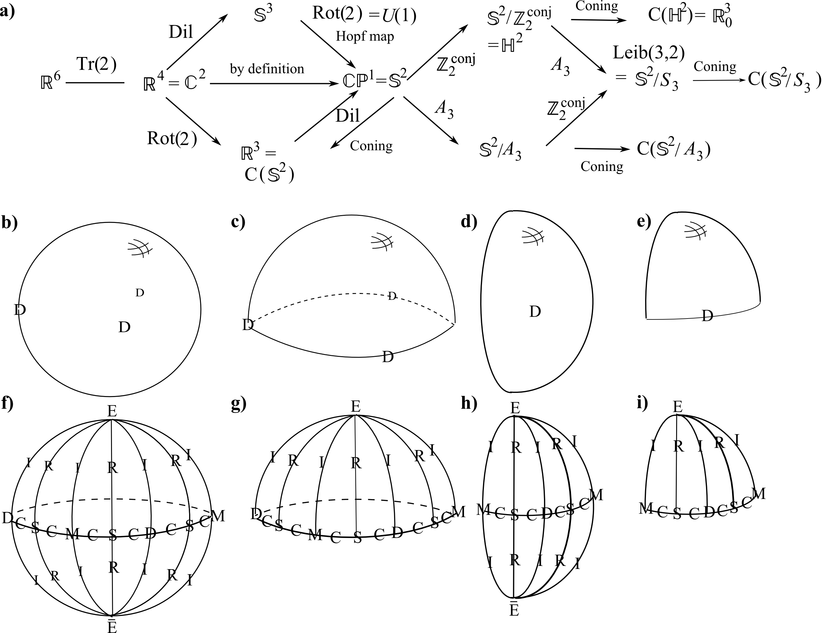
Figure 4: a) The sequence of configuration spaces for triangleland. $\mathbb{H}^{2}$ is the hemisphere with edge and $\mathbb{R}^{3}_{0}$ the half-space with edge. b), c), d) and e) are the configuration spaces for, respectively, the distinguishable particle plain shape case, the distinguishable particle mirror-image-identified shape case, the indistinguishable particle plain shape case and the indistinguishable particle mirror-image-identified shape case at the topological level. f), g), h) and i) are the tessellation for the distinguishable particle plain shape case, the distinguishable particle mirror-image-identified shape case, the indistinguishable particle plain shape case and the indistinguishable particle mirror-image-indentified shape case at the metric level.

The configuration space here for distinguishable particles and in the plain shape case is the sphere, decorated as in Figs 4b) and 4f). The labelled points and edges have the following geometrical/mechanical interpretations. E and $\bar{\mbox{E}}$ are the two mirror images of labelled equilateral triangles. C are arcs of the equator that is made up of collinear configurations. This splits the triangleland shape sphere into two hemispheres of opposite orientation (clockwise and anticlockwise labelled triangles, as in Fig 5c). Then it is clear that mirror-image-identification of shapes in space becomes, in the triangleland shape space, reflection in about the equator, a concept which immediately generalizes to $N$ particles if reinterpreted as the complex conjugation operation. This produces the hemisphere with edge, $\mathbb{H}^{2}$ [Fig 4c)], the cone over this then is $\mathbb{R}^{3}_{0}$: the half-space with edge. The I are bimeridians of isoscelesness with respect to the 3 possible clusterings (i.e. choices of apex particle and base pair). Each of these separates the triangleland shape sphere into hemispheres of right and left slanting triangles with respect to that choice of clustering [Fig 5b)]. The R are bimeridians of regularness (equality of the 2 partial moments of inertia of the each of the possible 2 constituent subystems: base pair and apex particle.) Each of these separated the triangleland shape sphere into hemispheres of sharp and flat triangles with respect to that choice of clustering [Fig 5a)]. The M are merger points: where one particle lies at the centre of mass of the other two. S denotes spurious points, which lie at the intersection of R and C but have no further notable properties (unlike the D, M or E points that lie on the other intersections).

Indistinguishability then involves quotienting out $S_{3}\,\,\ \widetilde{=}\,\,\mathbb{D}_{3}$ (permutations of the particles, isomorphic to the dihaedral group acting on the triangle of double collision points D and distinguishing the 2 hemispheres) [Fig 4e) and 4i)]. If mirror-image identification is absent, rather one quotients out $A_{3}\,\,\widetilde{=}\,\,\mathbb{Z}_{3}$ (even permutations of the particles, isomorphic to the cyclic group acting on the triangle of double collision points D) [Fig 4d) and 4h)].

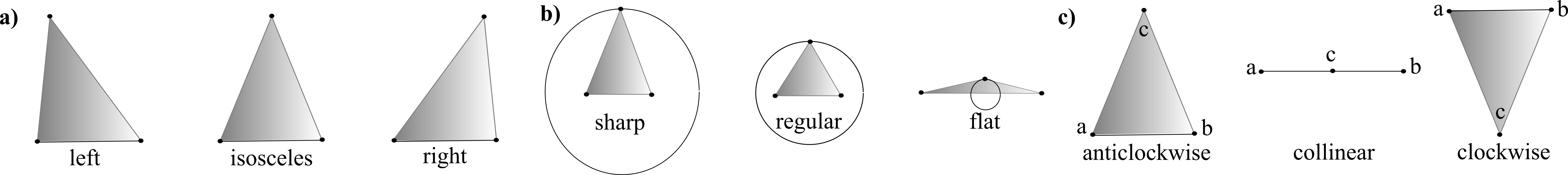
Figure 5: The most physically meaningful great circles on the triangleland shape correspond to the isosceles, regular and collinear triangles. These respectively divide the shape sphere into hemispheres of right and left triangles, sharp and flat triangles, and anticlockwise and clockwise triangles.

For later comparison with quadrilateralland,

1) useful redundant coordinates covering a surrounding Euclidean space (here also the relational space) are now the complicated combinations of the two Jacobi vectors, namely Dragt coordinates

$$\mbox{dra}_{1}=2\,{\mbox{\bf n}}_{1}\cdot{\mbox{\bf n}}_{2}\mbox{ }\mbox{ },\mbox{ }\mbox{dra}_{2}=2\{{\mbox{\bf n}}_{1}\mbox{\scriptsize{\bf$\mbox{ }\times\mbox{ }$}}{\mbox{\bf n}}_{2}\}_{3}\mbox{ }\mbox{ },\mbox{ }\mbox{dra}_{3}=|\mbox{n}_{2}|^{2}-|\mbox{n}_{1}^{2}|\mbox{ }.$$ (14)

These are, respectively [28], the anisoscelesness of the labelled triangle, four times the mass-weighted area of the triangle per unit moment of inertia and the ellipticity of the two partial moments of inertia. The area Dragt coordinate is a democratic invariant and is useable as a measure of uniformity [30], its modulus running from maximal value at the most uniform configuration (the equilateral triangle) to minimal value for the collinear configurations. The on-sphere condition is then $\sum_{\Delta=1}^{3}\mbox{dra}_{\Delta}\mbox{}^{2}=1$. These combinations appearing as surrounding Cartesian coordinates is much less obvious than the $\mbox{n}^{e}$ appearing in the same role for 4-stop metroland. These combinations arise from the sequence $\mathbb{R}^{4}\longrightarrow\mathbb{S}^{3}\longrightarrow\mathbb{S}^{2}\longrightarrow\mathbb{R}^{3}$, where the first map is an obvious on-sphere condition for preshape space within relative space, the second is mathematically the Hopf map and here sends preshape space to shape space, and the third is an obvious coning that here sends shape space to relative space.

2) One sometimes also swaps the dra₂ = demo(3) (the democratic invariant shape quantity for triangleland) for the scale variable $I$ in the non-normalized version of the coordinates to obtain the {$I$, aniso, ellip} system.

3) Then a simple linear recombination of this is {$I_{1}$, $I_{2}$, aniso}, i.e. the two partial moments of inertia and the dot product of the two Jacobi vectors. This is in turn closely related [7] to the parabolic coordinates on the flat $\mathbb{R}^{3}$ conformal to the triangleland relational space, which are $\{I_{1},I_{2},\Phi\}$.

4) Useful intrinsic coordinates are $\Theta$ and $\Phi$. These are again spherical polars, but their meaning in terms of the relative particle cluster separations is rather different. The interpretation of the azimuthal angle is now

$$\Theta=2\,\mbox{arctan}(\rho_{2}/\rho_{1})\mbox{ },$$ (15)

and that of the polar angle $\Phi$ is as in Fig 1d).

5 Quadrilateralland

5.1 Overview of configuration spaces for quadrilateralland

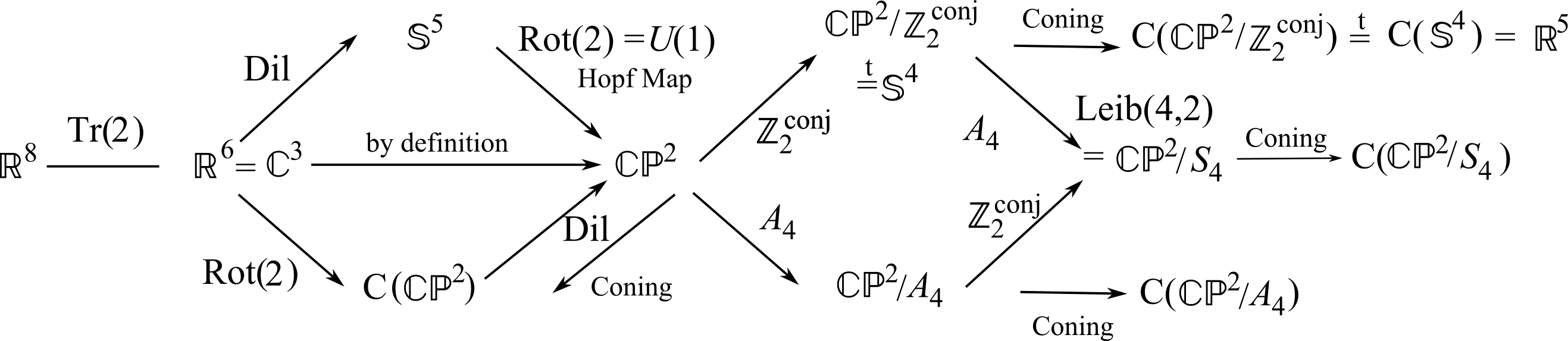
Figure 6: The sequence of configuration spaces for quadrilateralland. $\stackrel{{\scriptstyle t}}{{=}}$ denotes equality at the topological level.

N.B. this is harder to visualise than the previous subsections’ shape spaces, due to greater dimensionality as well as greater geometrical complexity and a larger hierarchy of special regions of the various possible codimensions. Geometrical detail of this space is in part built up in later Subsections.

Firstly, at the topological level, in the distinguishable particle plain shape case, the shape space is a $\mathbb{CP}^{2}$ decorated by a net of 6 $\mathbb{S}^{2}$ trianglelands (in each case with one vertex being a double collision corresponding to the $\mbox{\Large(}\stackrel{{\scriptstyle\mbox{\scriptsize 4}}}{{\mbox{\scriptsize 2}}}\mbox{\Large)}$ pairs of particles coinciding); each of these is an $\mathbb{S}^{2}$. There is also a net of 3-stop metrolands with one being a D point on an $\mathbb{RP}^{n}$ mirror image identified by rotation in 2-$d$, with further special T and DD points the usual 4 and 3 for a mirror-image identified such, and in the same pattern as in Fig 3. In the distinguishable particle mirror image identified case, the shape space is a $\mathbb{CP}^{2}/\mathbb{Z}_{2}^{\mbox{\scriptsize c}\mbox{\scriptsize o}\mbox{\scriptsize n}\mbox{\scriptsize j}}$ (see [44] for similar quotients but with a different meaning to the $\mathbb{Z}_{2}$ action) decorated by a net of 6 $\mathbb{RP}^{2}$ s trianglelands. In the indistinguishable particle plain shape case, the shape space is $\mathbb{CP}^{2}/A_{4}$, with the triangular configurations feeling only $A_{3}$. In the indistinguishable particle mirror-image-identified case, the shape space is $\mathbb{CP}^{2}/S_{4}$, with the triangular configurations feeling only $S_{3}$ but the $\mathbb{RP}^{2}$ of collinear configurations feeling the full $S_{4}$.

Secondly, at the metric level, collinearities become meaningful. These form $\mathbb{RP}^{2}$ in the distinguishable particle cases and $\mathbb{RP}^{2}/A_{4}$ in the indistinguishable particle cases. Here is a demonstration that $\mathbb{RP}^{N-2}$ plays this role within the general $N$-a-gonland $\mathbb{CP}^{N-2}$ case. Collinear configurations involve the relative angle coordinates being 0 or multiples of $\pi$, by which the complex projective space definition collapses to the real projective space definition (for which the ${\cal R}^{e}$ are Beltrami coordinates). Moreover, we know that abcd… can be rotated via the second dimension into …dcba (and that there is no further such identification) and so the real submanifold of collinear configurations is $\mathbb{RP}^{N-2}$. The above spaces of collinearity are in each case like an equator in each case, e.g. separating two $\mathbb{S}^{4}$’s in $\mathbb{E}^{5}$ in the first case (see below for why the two halves are, topologically, $\mathbb{S}^{4}$ and for further issues of the geometry involved).

Finally, there are also 6, 3, 2 and 1 distinguishable labelled squares in each case. This motivates a new action on quadrilateralland, in which e.g. the left-most particle is preserved and the other 3 are permuted or just evenly-permuted.

It is also easy to write conditions in these coordinates for rectangles, kites, trapezia, rhombi… but these are less meaningful 1) from a mathematical perspective (e.g. they are not topologically defined). 2) From a physical perspective (the square is additionally a configuration for which various notions of uniformity are maximal). However, squares are not the only notion of maximal uniformity by [30]’s the $s_{6}$ =demo(4) quantifier described in Sec 5.2; I further investigate this quantifier of uniformity using the present paper’s coordinate systems in Sec 5.5. Parallelograms also play a role in Figure 7.

5.2 Useful coordinate systems for quadrilateralland.

Further useful coordinate systems for quadrilateralland are as follows [these parallel the same 1) to 4) labels as in Sec 4].

1) {$s_{\Delta}$} are a redundant set of six shape coordinates (see [30] for their explicit forms), which are the quadrilateralland analogue of triangleland’s Dragt coordinates according to the construction in [33, 30].

2) However, for quadrilateralland, swapping one of the $s_{\Delta}$ [$s_{6}$ = demo($4$), a democracy invariant and proportional to the square root of the sum of the squares of the mass-weighted areas per unit MOI of the three coarse-graining triangles and parallelogram of Fig 7b-d) and g-i)] for a scale variable to form the coordinate system {$I$, $s_{\delta}$} turns out to give a more useful set [30].

3) Kuiper’s coordinates are then a simple linear combination of 2) (mixing the $I$, $s_{1}$ and $s_{5}$ coordinates). These consist of all the possible inner products between pairs of Jacobi vectors, i.e. 3 magnitudes of Jacobi vectors per unit MOI $N^{e}$, alongside 3 $\mbox{\bf n}_{f}\cdot\mbox{\bf n}_{g}$ ($e\neq f$), which are very closely related to the three relative angles. As such, they are, firstly, very much an extension of the parabolic coordinates for the conformally-related flat $\mathbb{R}^{3}$ of triangleland [7]. Secondly, in the quadrilateralland setting, they are a clean split into 3 pure relative angles (of which any 2 are independent and interpretable as the anioscelesnesses of the coarse-graining triangles or arhombicness of the coarse-graining parallelogram) and 3 magnitudes (supporting 2 independent non-angular ratios). I therefore denote this coordinate system by {$N^{e}$, aniso($e$)}. Thirdly, whilst they clearly contain 2 redundancies, they are fully democratic in relation to the constituent Jacobi vectors and coarse-graining triangles/parallelogram made from pairs of them.

Figure 7: Figure of the coarse-graining triangles. a) For Jacobi H-coordinates coordinates for a given quadrilateral, collapsing each of $\rho_{1}^{(\mbox{\tiny H}2)}$, $\rho_{2}^{(\mbox{\tiny H}2)}$ and $\rho_{3}^{(\mbox{\tiny H}2)}$ in turn gives the coarse-graining triangles b), c) and d) [30]. [One can use d) to interpret the associated anisoscelesness, but the true physical situation is that of e) i.e. a parallelogram.] Moreover, whilst both the triangles and the parallelograms have spheres for their reduced configuration spaces, the detail of how the sphere of parallelograms is decorated differs from how the sphere of triangles is decorated, so that one really needs to use e) itself. Then the analogue of anisoscelessness here is arhombicness, i.e. departure from the rightness of the angle of intersection of the diagonals that characterizes a rhombus.] If one uses Jacobi K-coordinates instead [f), new to this paper], then collapsing each of $\rho_{1}^{(\mbox{\tiny K}3)}$, $\rho_{2}^{(\mbox{\tiny K}3)}$ and $\rho_{3}^{(\mbox{\tiny K}3)}$ in turn gives the coarse-graining triangles g), h) and i). j) The anisoscelesness per unit base length is the amount by which the perpendicular to the base fails to bisect it is $l_{1}-l_{2}$ for $l_{1}$ and $l_{2}$ as indicated.

4) Useful intrinsic coordinates (which extend the spherical coordinates on the triangleland and 4-stop metroland shape spheres) are the Gibbons–Pope type coordinates {$\chi$, $\beta$, $\phi$, $\psi$} are also useful in this paper. The coordinate ranges are $0\leq\chi\leq\pi/2$, $0\leq\beta\leq\pi$, $0\leq\phi\leq 2\pi$ (a reasonable range redefinition since it is the third relative angle), and $0\leq\psi\leq 4\pi$. These are related to the bipolar form of the Fubini–Study coordinates by

$$\psi^{\prime}=-\{\Phi_{1}+\Phi_{2}\}\mbox{ },\mbox{ }\mbox{ }\phi^{\prime}=\Phi_{2}-\Phi_{1},$$ (16)

with then $\psi=-\psi^{\prime}$ (measured in the opposite direction to match Gibbons–Pope’s convention) and $\phi$ is taken to cover the coordinate range $0$ to $2\pi$, which is comeasurate with it itself being the third relative angle between the Jacobi vectors involved. However now in each of the conventions I use for H and K coordinates, a different interpretation is to be attached to these last two formulae in terms of the $\rho^{e}$. For H-coordinates in my convention,

$$\beta=2\,\mbox{arctan}\,(\rho_{2}/\rho_{1})\mbox{ },\mbox{ }\mbox{ }\chi=\mbox{arctan}\big{(}\sqrt{\rho_{1}\mbox{}^{2}+\rho_{2}\mbox{}^{2}}/\rho_{3}\big{)}\mbox{ },$$ (17)

whilst for K-coordinates in my convention,

$$\beta=2\,\mbox{arctan}\,(\rho_{1}/\rho_{2})\mbox{ },\mbox{ }\mbox{ }\chi=\mbox{arctan}\big{(}\sqrt{\rho_{1}\mbox{}^{2}+\rho_{2}\mbox{}^{2}}/\rho_{3}\big{)}\mbox{ }.$$ (18)

By their ranges, $\beta$ and $\phi$ parallel azimuthal and polar coordinates on the sphere. [In fact, $\beta$, $\phi$ and $\psi$ take the form of Euler angles on $SU(2)$, with the remaining coordinate $\chi$ playing the role of a compactified radius.] Now, in the quadrilateralland interpretation, $\beta$ has the same mathematical form as triangleland’s azimuthal coordinate $\Theta$ (15). Additionally, $\chi$ parallels 4-stop metroland’s azimuthal coordinate $\theta$ [the first equation in (12)], except that it is over half of the range of that, reflecting that the collinear 1234 and 4321 orientations have to be the same due to the existence of the second dimension via which one is rotateable into the other.

The Gibbons–Pope type coordinates have the following quadrilateralland interpretations. In an H-clustering, the $\phi$ is the difference of the relative angles [see Fig 2e)], so the associated momentum represents a counter-rotation of the two constituent subsystems ($\times$ relative to {12} and + relative to {34}). The $\psi$ is minus the sum of the relative angles, so the associated momentum represents a co-rotation of these two constituent subsystems (with counter-rotation in $\times$ relative to $+$ so as to preserve the overall zero angular momentum condition). The $\beta$ is a measure of contents inhomogeneity of the model universe: the ratio of the sizes of the 2 constituent subclusters. Finally, the $\chi$ is a measure of the selected subsystems’ sizes relative to that of the whole-universe model. These last two are conjugate to quantities that involve relative dilational momenta in addition to relative angular momenta.

On the other hand, in a K-clustering, the $\phi$ is the difference of the two relative angles [see Fig 2f)], but by the directions these are measured in, the associated momentum now represents a co-rotation of the two constituent subsystems (which are now {12} relative to 4 and {+4} relative to 3, and with counter-rotation in T relative to $+$ so as to preserve the overall zero angular momentum condition). The $\psi$ is minus the sum of the two relative angles, so the associated momentum represents a counter-rotation of these two constituent subsystems. The $\beta$ is now a comparer between the sizes of the {12} subcluster and the separation between the non-triple cluster particle 3 and T. Finally, the $\chi$ is a comparer between the sizes of the above two contents of the universe ({12} and {T3}) on the one hand, and the separation between them on the other hand ({4+}, which is a measure of separation of {12} and {T3}). These last two are again conjugate to quantities that involve relative dilational momenta in addition to relative angular momenta. Note how in both H and K cases, the Gibbons–Pope type coordinates under the quadrilateralland interpretation involve a split into two pure relative angles and two pure non-angular ratios of magnitudes.

In Gibbons–Pope type coordinates, the Fubini–Study metric then takes the form

$$\textrm{d}s^{2}=\textrm{d}\chi^{2}+\mbox{sin}^{2}\chi\big{\{}\textrm{d}\beta^{2}+\mbox{cos}^{2}\chi\{\textrm{d}\phi^{2}+\textrm{d}\psi^{2}+2\,\mbox{cos}\,\beta\,\textrm{d}\phi\textrm{d}\psi\}+\mbox{sin}^{2}\chi\,\mbox{sin}^{2}\beta\,\textrm{d}\phi^{2}\big{\}}/4\mbox{ },$$ (19)

leading to a kinetic term

$$\mbox{T}=\dot{\chi}^{2}/2+\mbox{sin}^{2}\chi\big{\{}\dot{\beta}^{2}+\mbox{cos}^{2}\chi\{\dot{\phi}^{2}+\dot{\psi}^{2}+2\,\mbox{cos}\,\beta\,\dot{\phi}\dot{\psi}\}+\mbox{sin}^{2}\chi\,\mbox{sin}^{2}\beta\,\dot{\phi}^{2}\big{\}}/8\mbox{ }.$$ (20)

5.3 The inclusion of trianglelands and 4-stop metroland within quadrilateralland

In Gibbons–Pope type coordinates based on the Jacobi H, when $\rho_{3}=0$, $\chi=\pi/2$ and the metric reduces to

$$\textrm{d}s^{2}=\{1/2\}^{2}\{\textrm{d}\beta^{2}+\mbox{sin}^{2}\beta\,\textrm{d}\phi^{2}\}$$ (21)

i.e. a sphere of radius 1/2, which corresponds to the conformally-untransformed $\mathbb{CP}^{1}$. When $\rho_{2}$ = 0, $\beta=0$ and the metric reduces to

$$\textrm{d}s^{2}=\{1/2\}^{2}\{\textrm{d}\Theta_{1}^{2}+\mbox{sin}^{2}\Theta_{1}\textrm{d}\Phi_{1}^{2}\}$$ (22)

for $\Theta_{1}=2\chi$ having the correct coordinate range for an azimuthal angle. Finally, when $\rho_{1}$ = 0, $\beta=0$ and the metric reduces to

$$\textrm{d}s^{2}=\{1/2\}^{2}\{\textrm{d}\Theta_{2}^{2}+\mbox{sin}^{2}\Theta_{2}\textrm{d}\Phi_{2}^{2}\}$$ (23)

for $\Theta_{2}=2\chi$ again having the correct coordinate range for an azimuthal angle. The first two of these spheres are a triangleland shape sphere included within quadrilateralland as per Sec 5.1. The first is for {12}, 4 and 3 as the particles. The second is for 1, 2 and 34 as the particles. The third of these spheres corresponds, rather, to a merger, of + and $\times$, i.e. a merger of type $\mbox{M}^{\mbox{\scriptsize D}\mbox{\scriptsize D}}$ – the space of parallelograms labelled as in Fig 7e).

In Gibbons–Pope type coordinates based on the Jacobi K, when $\rho_{3}=0$, $\chi=\pi/2$ and the metric reduces to

$$\textrm{d}s^{2}=\{1/2\}^{2}\{\textrm{d}\beta^{2}+\mbox{sin}^{2}\beta\,\textrm{d}\phi^{2}\}$$ (24)

i.e. a sphere of radius 1/2, which corresponds to the conformally-untransformed $\mathbb{CP}^{1}$. When $\rho_{2}$ = 0, $\beta=0$ and the metric reduces to

$$\textrm{d}s^{2}=\{1/2\}^{2}\{\textrm{d}\Theta_{1}^{2}+\mbox{sin}^{2}\Theta_{1}\textrm{d}\Phi_{1}^{2}\}$$ (25)

for $\Theta_{1}=2\chi$ again having the correct coordinate range for an azimuthal angle. Finally, when $\rho_{1}$ = 0, $\beta=0$ and the metric reduces to

$$\textrm{d}s^{2}=\{1/2\}^{2}\{\textrm{d}\Theta_{2}^{2}+\mbox{sin}^{2}\Theta_{2}\textrm{d}\Phi_{2}^{2}\}$$ (26)

for $\Theta_{2}=2\chi$ yet again having the correct coordinate range for an azimuthal angle. The second of these is a triangleland shape space sphere with 12, 4 and 3 as the particles. The first and third correspond rather to mergers, of +, T and 4 in the first case (of type $\mbox{M}^{\mbox{\scriptsize T}}\cap\mbox{M}^{\mbox{\scriptsize D}\mbox{\scriptsize D}}$), and of T and 3 in the second case (of type $\mbox{M}^{\mbox{\scriptsize T}}$).

In Kuiper coordinates, each of the three on-$\mathbb{S}^{2}$ conditions for whichever of H or K coordinates involves losing one magnitude and two inner products. Thus the survivors are two magnitudes and one inner product (closely related to parabolic coordinates and linearly combineable to form the {$I$, aniso, ellip} system, see Sec 4). If we recombine the Kuiper coordinates to form the {$I,s_{\delta}$} system, and swap the $I$ for the $s_{6}$ = demo(4), then the survivors of the procedure are the Dragt coordinates (since the procedure kills two of the three area contributions to the $s_{6}$). This gives another sense in which the {$s_{\Delta}$} system is a natural extension of the Dragt system.

5.4 The split into hemi-$\mathbb{CP}^{2}$’s of oriented quadrilaterals

Definition: The Veronese surface $V$ [45] is the space of conics through a point (parallel to how a projective space is a set of lines through a point).

Kuiper’s Theorem i) The map

$$\eta:\stackrel{{\scriptstyle\mbox{$\mathbb{CP}^{2}$}}}{{(\mbox{z}_{1},\mbox{z}_{2},\mbox{z}_{3})}}\mbox{ }\mbox{ }\mbox{ }\stackrel{{\scriptstyle\mbox{$\longrightarrow$}}}{{\stackrel{{\scriptstyle}}{{\mbox{$\longmapsto$}}}}}\mbox{ }\mbox{ }\mbox{ }\stackrel{{\scriptstyle\mbox{$\mathbb{E}^{5}$}}}{{(|\mbox{z}_{1}|^{2},|\mbox{z}_{2}|^{2},|\mbox{z}_{3}|^{2},\{\mbox{z}_{2}\bar{z}_{3}+\mbox{z}_{3}\bar{z}_{2}\}/2,\{\mbox{z}_{3}\bar{z}_{1}+\mbox{z}_{1}\bar{z}_{3}\}/2,\{\mbox{z}_{1}\bar{z}_{2}+\mbox{z}_{2}\bar{z}_{1}\}/2)}}$$ (27)

induces a piecewise smooth embedding of $\mathbb{CP}^{2}/\mathbb{Z}_{2}^{\mbox{\scriptsize c}\mbox{\scriptsize o}\mbox{\scriptsize n}\mbox{\scriptsize j}}$ onto the boundary of the convex hull of the Veronese surface $V$ in $\mathbb{E}^{5}$, which moreover has the right properties to be the usual smooth 4-sphere [36].

N.B. this is at the topological level; it clearly cannot extend to the metric level by a mismatch in numbers of Killing vectors ($\mathbb{S}^{4}$ with the standard spherical metric has 10 whilst $\mathbb{CP}^{2}$ equipped with the Fubini–Study metric has 8).

Restricting $\{{\mbox{z}}_{1},{\mbox{z}}_{2},{\mbox{z}}_{3}\}$ to the real line corresponds in the quadrilateralland interpretation to considering the collinear configurations, which constitute a $\mathbb{RP}^{2}$ space as per Sec 5.1 Moreover the above embedding sends this onto the Veronese surface $V$ itself. Proving this proceeds via establishing that, as well as the on-$\mathbb{S}^{5}$ condition $N_{1}+N_{2}+N_{3}=1$, a second restriction holds, which in our quadrilateralland interpretation, reads $\sum_{e=1}^{n}\mbox{aniso}(e)^{2}N^{e}-4N_{1}N_{2}N_{3}+\mbox{aniso}(1)\,\mbox{aniso}(2)\,\mbox{aniso}(3)=0$. (Knowledge of this restriction should also be useful in kinematical quantization [46], and it is clearer in the {$N^{e}$, aniso($e$)} system, which is both the quadrilateralland interpretation of Kuiper’s redundant coordinates and a simple linear recombination of the {$I$,$s_{\delta}$} coordinates obtained in [30], than in these other coordinates themselves.)

Another form for Kuiper’s theorem [36]. Moreover, $\mathbb{CP}^{2}$ itself is topologically a double covering of $\mathbb{S}^{4}$ branched along the $\mathbb{RP}^{2}$ of collinearities which itself embeds onto $\mathbb{E}^{5}$ to give the Veronese surface $V$.

Here, branching is meant in the sense familiar from the theory of Riemann surfaces [47]. Moreover, the $\mathbb{RP}^{2}$ itself embeds non-smoothly into the Veronese surface $V$.

Then the quadrilateralland interpretation of these results is in direct analogy with the plain shapes case of triangleland consisting of two hemispheres of opposite orientation bounded by an equator circle of collinearity, the mirror-image-identified case then consisting of one half plus this collinear edge. Thus plain quadrilateralland s distinction between clockwise- and anticlockwise-oriented figures is strongly anchored to this geometrical split, with the collinear configurations lying at the boundary of this split.

5.5 Notions of uniformity cast in Kuiper and Gibbons–Pope coordinates

In this quadrilateralland case, there are then 3 squares in each hemi-$\mathbb{CP}^{2}$ as opposed to the single equilateral triangle in each hemisphere of triangleland; these are particularly uniform configurations. This reflects the presence of a further 3-fold symmetry in quadrilateralland; choosing to use indistinguishable particles then quotients this out.

As explained in detail in [28], the nontrivial democratic invariant demo(3) for triangleland is the mass-weighted area of the triangle per unit moment of inertia, and that for quadrilateralland, demo(4), is proportional to the square root of the sum of the mass-weighted areas of the coarse-graining triangles/parallelogram in Fig 7. Now, extremizing demo(3) invariant picks out the two labelled equilateral triangles, which is uniform in a very strong sense; on the other hand, extremizing demo(4) does pick out the six labelled squares, but nonuniquely – one gets one extremal curve per hemi-$\mathbb{CP}^{2}$. Now, the present paper’s choices of coordinate systems furthermore clarify the interpretation to be given to these two extremal curves. In $\{N^{e}$, aniso($e$)} coordinates, this is given by aniso(1) = 0 = aniso(2) and $\left|\mbox{aniso(3)}\right|$ = 1, i.e. (1)-isosceles, (2)-isosceles and maximally (3)-right or (3)-left i.e. (3)-collinear, with $N_{3}$ = 1/2 and $N_{1}$, $N_{2}$ varying (but such that the on-$\mathbb{S}^{5}$ condition $N_{1}+N_{2}+N_{3}=1$ holds). On the other hand, in Gibbons–Pope type coordinates, the uniformity condition is $\phi=0$, $\psi=4\pi$, $\chi=\pi/4$ and $\beta$ free, i.e., in the H-coordinates case, freedom in the contents inhomogeneity i.e. size of subsystem 1 relative to the size of subsystem 2. On the other hand, in the K-coordinates case, $\beta$ free signifies freedom in how tall one makes the selected {12, 3} cluster’s triangle.

6 Conclusion

6.1 Outline of the results so far

Quadrilateralland’s shape space is $\mathbb{CP}^{2}$ or some quotient of this by a discrete group. I considered this for plain and mirror-image identified choices of shapes, and for distinguishable and indistinguishable particles. In the case in which distinct particle masses do not naturally label the particles as distinct, the most Leibnizian shape space is Leib$(4,2)=\mathbb{CP}^{2}/S_{4}$. I have also explained how trianglelands and 4-stop metrolands occur within quadrilateralland; these correspond at the level of space to double collision configurations and collinear configurations. At the level of configuration spaces, they correspond respectively to $\mathbb{S}^{2}$’s or quotients and to $\mathbb{RP}^{2}$’s or quotients. I have also drawn attention to Kuiper’s theorem as providing, in the present quadrilateralland context, the analogue of the 2 hemispheres of orientation separated by an equator of collinearity for triangleland and the codimension-1 embedding thereof into a surrounding Euclidean space. This paper was also the first to present details of the Jacobi K-coordinate study of 4-stop metroland and quadrilateralland, and of the structure of the set of mergers for 4-stop metroland and quadrilateralland.

I identified the following coordinate systems as useful for the study of quadrilateralland.

1) Kuiper coordinates (a redundant presentation on $\mathbb{C}^{3}$). These consist of magnitudes of the 3 mass-weighted Jacobi vectors and the 3 inner products between these vectors. These are then physically interpreted as the three partial moments of inertia of the system and the three anisoscelesneses of Fig 7’s coarse-graining triangles (with one substituted for an arhombicness of a parallelogram in the H case) obtained from the quadrilateral by striking out each Jacobi vector in turn. These are closely related to triangleland’s conformally-related flat space’s parabolic coordinates: two partial moments of inertia and the relative angle between the two Jacobi vectors.

2) Gibbons–Pope type coordinates, which, for quadrilateralland in an H-clustering, are to be identified as a difference of relative angles, minus the sum of the relative angles, a measure of contents inhomogeneity and a measure of the selected subsystems’ sizes relative to that of the whole-universe model. In K-coordinates, the last two are, rather, i) a comparer between the sizes of the {12} subcluster and the separation between the non-triple cluster particle 3 and T, and ii) a comparer between the sizes of the above two contents of the universe ({12} and {T3}) on the one hand, and the separation between them on the other hand ({4+}, which is a measure of separation of {12} and {T3}).

In H-coordinates, the momentum associated with the difference of relative angles represents a counter-rotation of the two constituent subsystems ($\times$ relative to {12} and + relative to {34}), while the momentum associated with the sum of relative angles represents a co-rotation of these two constituent subsystems (with counter-rotation in $\times$ relative to $+$ so as to preserve the overall zero angular momentum condition). On the other hand, in K-coordinates, the momentum associated with a difference of relative angles represents a co-rotation of the two constituent subsystems (which are now {12} relative to 4 and {+4} relative to 3, and with counter-rotation in T relative to $+$ so as to preserve the overall zero angular momentum condition), whilst that associated with the sum of relative angles represents a counter-rotation of these two constituent subsystems. These momenta will turn out to play an important role in the study of conserved quantities in quadrilateralland [34].

Square configurations and a weaker criterion of uniform states based on the extremization of the sum of the squares of the mass-weighted areas per unit MOI of the three coarse-graining triangles (or two triangles and one parallelogram) were furtherly understood using this paper’s coordinate systems.

6.2 Generalizations of this paper

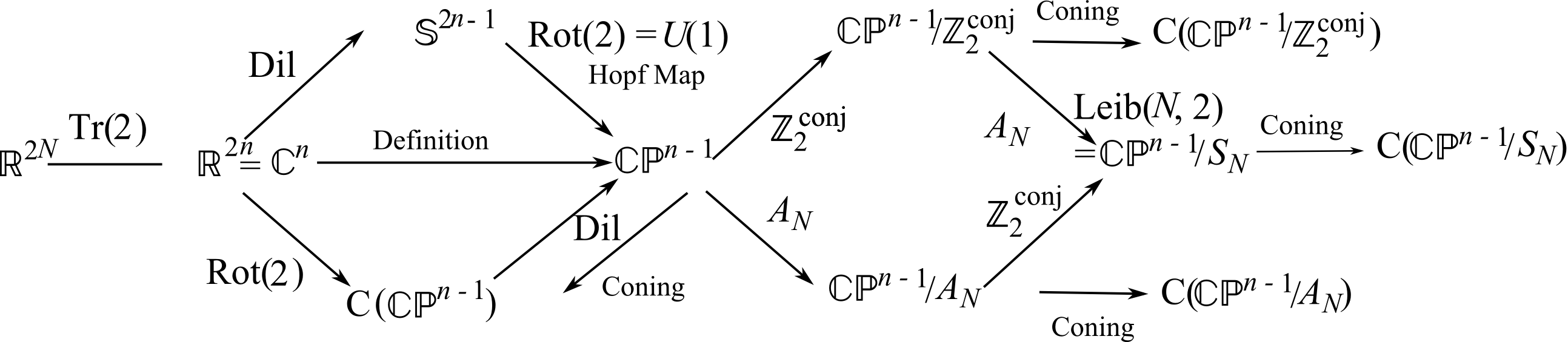
Figure 8: The sequence of configuration spaces for $N$-a-gonland.

Extending the Dragt/parabolic/shape/Kuiper type of redundant coordinates is itself straightforward, though it is not clear the extent to which the resulting coordinates will retain usefulness for the study of each $\mathbb{CP}^{N-2}$. Certainly the number of Kuiper-type coordinates (based on inner products of pairs of Jacobi vectors, of which there are $N\{N-1\}/2$) further grows away from 2$N$ = dim($\mathbb{CP}^{\mbox{\scriptsize N}}$) as $N$ gets larger. The present paper also finds a surrounding space of just one dimension more for $\mathbb{CP}^{2}$. The $N$-a-gonland significance of two half-spaces of different orientation separated by an orientationless manifold of collinearities gives reason for double covers to the $N-2\geq 3$ $\mathbb{CP}^{N-2}$ spaces to exist for all $N$. However, there is no known guarantee that these will involve geometrical entities as simple as or tractable as quadrilateralland’s $\mathbb{S}^{4}$ for the half-spaces, or of the Veronese surface $V$ as the place of branching. However, one does have the simple argument of Sec 5.1 that the manifold of collinearities within $N$-a-gonland’s $\mathbb{CP}^{N-2}$ is $\mathbb{RP}^{N-2}$, so at least that is a known and geometrically-simple result for the structure of the general $N$-a-gonland. Whether the intrinsic Gibbons–Pope type coordinates can be extended to $N$-a-gonland in a way that maintains their usefulness in characterizing conserved quantities [34] and via separating the free-potential time-independent Schrödinger equation, remains to be seen.

As regards the Quantum Information Theory counterpart of this work, one possible usefulness of representing qtrit states as quadrilaterals is via the convenience of having a 2-$d$ graphical representation, which, moereover, remains 2-$d$ as one passes to the study of q$n$its. In this picture, the relation between the 3 included $SU(2)$ ladders and the 3 coarse-graining triangles (or two triangles and one parallelogram) is that there are 3 constituent (overlapping) qbits in a qtrit. I leave what the Gibbons–Pope and Kuiper coordinates (and the associated democratic invariant) signify in the study of Qutrits as an interesting open question in parallel to the present paper.

6.3 RPM’s and Problem of Time strategies

Some of the strategies toward resolving the Problem of Time in Quantum Gravity modellable by RPM’s are as follows [43].

A) Perhaps one has slow heavy ‘$h$’ variables that provide an approximate timestandard with respect to which the other fast light ‘$l$’ degrees of freedom evolve [48, 26, 15, 16]. In the Halliwell–Hawking [26] scheme for GR Quantum Cosmology, $h$ is scale (and homogeneous matter modes) and $l$ are small inhomogeneities. Thus the scale–shape split of scaled RPM’s afford a tighter parallel of this [19, 49, 50] than pure-shape RPM’s. The semiclassical approach involves firstly making the Born–Oppenheimer ansatz $\Psi(h,l)=\psi(\mbox{h})|\chi(h,l)\rangle$ and the WKB ansatz $\psi(h)=\mbox{exp}(iW(h)/\hbar)$. Secondly, one forms the $h$-equation ($\langle\chi|\widehat{H}\Psi=0$ for RPM’s), which, under a number of simplifications, yields a Hamilton–Jacobi equation

$$\{\partial W/\partial h\}^{2}=2\{\mbox{E}-\mbox{V}(h)\}\mbox{ }$$ (28)

for $\mbox{V}(h)$ the $h$-part of the potential. Thirdly, one way of solving this is for an approximate emergent semiclassical time $t^{\mbox{\scriptsize e}\mbox{\scriptsize m}}=t^{\mbox{\scriptsize e}\mbox{\scriptsize m}}(h)$. Next, the $l$-equation $\{1-|\chi\rangle\langle\chi|\}\widehat{{\cal H}}\Psi=0$ can be recast (modulo further approximations) into an emergent-time-dependent Schrödinger equation for the $l$ degrees of freedom

$$i\hbar\partial|\chi\rangle/\partial t^{\mbox{\tiny e}\mbox{\tiny m}}=\widehat{H}_{l}|\chi\rangle\mbox{ }.$$ (29)

(Here the left-hand side arises from the cross-term $\partial_{h}|\chi\rangle\partial_{h}\psi$ and $\widehat{H}_{l}$ is the remaining surviving piece of $\widehat{H}$). Note that the working leading to such a time-dependent wave equation ceases to work in the absense of making the WKB ansatz and approximation, which, additionally, in the quantum-cosmological context, is not known to be a particularly strongly supported ansatz and approximation to make.

B) A number of approaches take timelessness at face value. One considers only questions about the universe ‘being’, rather than ‘becoming’, a certain way. This has at least some practical limitations, but can address some questions of interest. As a first example, the naïve Schrödinger interpretation [51] concerns the ‘being’ probabilities for universe properties such as: what is the probability that the universe is large? Flat? Isotropic? Homogeneous? One obtains these via consideration of the probability that the universe belongs to region R of the configuration space that corresponds to a quantification of a particular such property,

$$\mbox{Prob(R)}\propto\int_{\mbox{\scriptsize R}}|\Psi|^{2}\textrm{d}\Omega\mbox{ },$$ (30)

for $\textrm{d}\Omega$ the configuration space volume element. As a second example, the conditional probabilities interpretation [52] goes further by addressing conditioned questions of ‘being’ such as ‘what is the probability that the universe is flat given that it is isotropic’? As a final example, records theory [52, 53, 5, 54, 20] involves localized subconfigurations of a single instant. More concretely, it concerns whether these contain useable information, are correlated to each other, and a semblance of dynamics or history arises from this. This requires notions of localization in space and in configuration space as well as notions of information. RPM’s are superior to minisuperspace for such a study as, firstly, they have a notion of localization in space. Secondly, they have more options for well-characterized localization in configuration space (i.e. of ‘distance between two shapes’ [43]) through their kinetic terms possessing positive-definite metrics.

C) Perhaps instead it is the histories that are primary (histories theory [53, 55]).

Combining A) to C) (for which RPM’s are well-suited) is a particularly interesting prospect [56], along the following lines (see also [53, 54, 57, 43] for further development of this). There is a records theory within histories theory. Histories decohereing is one possible way of obtaining a semiclassical regime in the first place, i.e. finding an underlying reason for the crucial WKB assumption without which the semiclassical approach does not work. What the records are will answer the also-elusive question of which degrees of freedom decohere which others in Quantum Cosmology.

(Observables-based approaches [6] can also be studied in the RPM arena, as can be quantum cosmologically aligned hidden time approaches for scaled RPM’s.)

6.4 Use of regions of configuration space in Problem of Time approaches

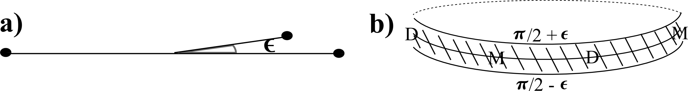
Figure 9: a) $\epsilon$-collinearity in space for three points. b) The corresponding configuration space belt of width 2$\epsilon$.

Next, I consider the role of configuration space regions in a number of these approaches. I find that Gibbons–Pope type coordinates are useful in considering regions of configuration space: the volume element is simple in these,

$\mbox{sin}^{3}\chi\mbox{cos}\,\chi\,\textrm{d}\chi\mbox{sin}\,\beta\,\textrm{d}\beta\,\textrm{d}\phi\,\textrm{d}\psi/8$, and so are characterizations for a number of physically and geometrically significant regions.

Application 1) To computing naïve Schrödinger interpretation probabilities of ‘being’, via (30). This is a continuation of what I have done in previous papers for metrolands and triangleland [21, 28, 18, 29]. Note the ‘sphere factor’ within this volume element (the $\beta$ and $\phi$ factors). The above gives

$$\mbox{Prob}(\mbox{Region R})\propto\int_{\mbox{\scriptsize R}}|\Psi(\chi,\beta,\phi,\psi)|^{2}\mbox{sin}^{3}\chi\mbox{cos}\,\chi\,\textrm{d}\chi\mbox{sin}\,\beta\,\textrm{d}\beta\,\textrm{d}\phi\,\textrm{d}\psi\mbox{ }.$$ (31)

Then both volume element and the wavefunctions (at least in the free potential case [58, 35]) separate into a product of factors $C(\chi)D(\beta)E(\phi)H(\psi)$, and also the region of integration (at least for a number of physically-significant regions including the below examples) so that the integration over configuration space reduces to a product of 1-$d$ integrals, rendering integration relatively straightforward.

The next issue addressed in this paper is to characterize some physically-significant R’s. [The wavefunctions themselves are provided in [35], where I combine them and this paper’s study of regions to also provide naïve Schrödinger interpretation probabilities for approximate-collinearity, approximate-squareness and approximate-triangularity.]

4-stop metroland and triangleland counterparts of such regions are e.g. caps, belts and lunes in spherical polar coordinates [21, 28] endowed with particular physical significance, such as the cap of $\epsilon$-equilaterality or the belt of

$\epsilon$-collinearity [Fig 8b)]. The present paper’s regions are somewhat more involved due to involving the more complicated and higher-dimensional geometry of $\mathbb{CP}^{2}$. One thing noted for the shape space spheres is a correspondence between the size of the region in question (e.g. the radius of a small cap, the width of a small belt, the angle of a narrow lune and combinations of these by union, intersection and negation) and the size of the departure in space from the precise configuration. E.g. the width of the belt of collinearity on the shape sphere corresponds to a Kendall type [14, 28] notion of $\epsilon$-collinearity of three points in space (Fig 8). Establishing such correspondences is then part of the study of physically-significant regions of the $\mathbb{CP}^{2}$ configuration space also. In particular, I consider the following.

I) Approximately-collinear quadrilaterals. Exactly collinear was $\mathbb{RP}^{2}$ corresponding to, in configuration space studied using H-coordinates, both angular coordinates $\phi$ and $\psi$ being 0 or an integer multiple of $\pi$. This condition is now $\epsilon$-relaxed. Thus the region of integration is all values of the ratio coordinates $\beta$ and $\chi$ whilst the angular coordinates are to live within the following union of products of intervals:

$$\big{(}\{0\leq\phi\leq\epsilon\}\cup\{\pi-\epsilon\leq\phi\leq\pi+\epsilon\}\cup\{2\pi-\epsilon\leq\phi\leq 2\pi\}\big{)}\times$$

$$\big{(}\{0\leq\psi\leq\epsilon\}\cup\{\pi-\epsilon\leq\psi\leq\pi+\epsilon\}\cup\{2\pi-\epsilon\leq\phi\leq 2\pi+\epsilon\}\cup\{3\pi-\epsilon\leq\phi\leq 3\pi+\epsilon\}\cup\{4\pi-\epsilon\leq\phi\leq 4\pi\}\big{)}\mbox{ }.$$ (32)

From the perspective of each configuration in space, this notion of $\epsilon$-collinearity corresponds to the relative angles $\Phi_{1}$ and $\Phi_{2}$ each lying within $[0,\epsilon]\cup[\pi-\epsilon,\pi+\epsilon]\cup[2\pi-\epsilon,2\pi]$.

II) Quadrilaterals that are approximately triangular or approximately one of the mergers depicted in the coarse-graining triangles or parallelogram of Fig 7. The exact configuration in each of these cases is a sphere characterized by one ratio variable and one relative angle variable. In moving away from exact triangularity, a second $\epsilon$-sized ratio variable becomes involved, and, in doing so one is rendering the other relative angle meaningful, allowing it to take all values. Thus the region of integration here is all angles, one ratio variable taking all possible values also, and the other being confined to an $\epsilon$-interval about the value that corresponds to exact triangularity. To be more concrete, consider the {+43} triangle in Gibbons–Pope type coordinates that derive from H-coordinates. Here, $\beta=\pi$, so the region of integration is all $\phi$, all $\psi$, all $\chi$ and $\pi-\epsilon\leq\beta\leq\pi$. Then, for example, the notion of $\epsilon$-{+43} triangular corresponds in space to the ratio {12}/{+$\times$} being of size $\epsilon/2$ or less.

III) One of the labellings of exact square configuaration is at $\phi=0$, $\psi=\pi$, $\beta=\pi/2$ and $\chi=\pi/4$. Approximate squareness allows for all four of these quantities to be $\epsilon$-close, so that the region of integration is a product of four intervals of width $\epsilon$ about these points. That corresponds to the two sides of the Jacobi H being allowed to be $\epsilon$-close ($\beta$-variation), the quadrilateral to vary in height to length ratio ($\chi$-variation) and for each of the sides of the Jacobi H to become non-right with respect to the cross-bar ($\psi$- and $\phi$-variation), which is an entirely intuitive parametrization of the possible small departures from exact squareness. [If one is interested in all of the labellings of the square, one can straightforwardly characterize each with a similar construction and again take the union of these regions.] This example is clearly furthermore useful as a notion of approximate uniformity, which is of interest in classical and quantum Cosmology.

Finally, note that if one considers mirror-image-identified and/or indistinguishable particles, then one has just a portion of $\mathbb{CP}^{2}$ in total and then the physically significant regions are smaller subsets (including sums over less things, e.g. there are now 3, 2 or just 1 distinct square configurations).

Application 2) The above notions of closeness and use of the Fubini–Study kinetic metric additionally embody control over localization both in space and in configuration space, allowing for the triangleland work towards establishing a records theory in [43] (concerning in particular notions of distance between shapes) to be extended to quadrilateralland.

Application 3) In the semiclassical approach, the many approximations used only hold in certain regions, in particular the crucial Born–Oppenheimer and WKB approximations. The semiclassical application awaits having the semiclassical approach sorted out for scaled quadrilateralland [35]; for the moment see [49] for the triangleland counterpart of such workings. This is needed for extending semiclassical work in [18, 29, 49] to the quadrilateralland setting.

Application 4) Regions also feature in the histories approach and in Halliwell’s combination of this with semiclassical approach and timeless ideas. Indeed, an extra connector between these approaches is that [56, 57] the semiclassical approach aids in the computation of timeless probabilities of histories entering given configuration space regions. This, by the WKB assumption, gives a wavefunction flux into each region in terms of W and the Wigner function (see e.g. [56]). Moreover, such schemes go beyond the standard semiclassical approach, so there is some chance that further objections to the semiclassical approach (problems inherited from the Wheeler–DeWitt equation and problems with reconstructing spacetime in such approaches) would be absent from the new unified strategy. I am presently considering extending [56] to RPM’s (for the moment for triangleland), looking at, without reference to time, what is the probability of finding the system in a series of regions of configuration space for a given eigenstate of the Hamiltonian [56]? Halliwell studied this with a free particle, a working which has a direct, and yet more genuinely closed-universe, counterpart for scaled triangleland [7] via the ‘Cartesian to Dragt coordinates correspondence’ allowing me to transcribe this working to a relational context. The quadrilateralland extension of this calculation, whilst remaining relationally interpretable as a closed-universe model, would represent a step-up in complexity and mathematical novelty for this program.

Acknowledgements: I thank those close to me for being supportive of me whilst this work was done. Professors Don Page and Gary Gibbons for teaching me about $\mathbb{CP}^{2}$. Dr Julian Barbour for introducing me to RPM s. Professors Gary Gibbons, Jonathan Halliwell, Chris Isham and Karel Kuchař for discussions. Mr Eduardo Serna for reading earlier drafts of this manuscript. Professors Belen Gavela, Marc Lachièze-Rey, Malcolm MacCallum, Don Page, Reza Tavakol, and Dr Jeremy Butterfield for support with my career. Fqxi grant RFP2-08-05 for travel money whilst part of this work was done in 2009-2010, and Universidad Autonoma de Madrid for funding in 2010–2011.

References

- [1]
- [2] J.B. Barbour and B. Bertotti, Proc. Roy. Soc. Lond. A382 295 (1982).
- [3] J.B. Barbour, Class. Quantum Grav. 20 1543 (2003), gr-qc/0211021.
- [4] J.B. Barbour, Class. Quantum Grav. 11 2853 (1994).
- [5] J.B. Barbour, The End of Time (Oxford University Press, Oxford 1999).
- [6] C. Rovelli, Quantum Gravity (Cambridge University Press, Cambridge 2004).
- [7] E. Anderson, Class. Quantum Grav. 26 135020 (2009), arXiv:0809.1168.
- [8] J.B. Barbour, B.Z. Foster and N. Ó Murchadha, Class. Quantum Grav. 19 3217 (2002), gr-qc/0012089; E. Anderson, Gen. Rel. Grav. 36 255, gr-qc/0205118; Phys. Rev. D68 104001 (2003), gr-qc/0302035; “Geometrodynamics: Spacetime or Space?” (Ph.D. Thesis, University of London 2004), gr-qc/0409123; E. Anderson, in General Relativity Research Trends, Horizons in World Physics 249 ed. A. Reimer (Nova, New York 2005), gr-qc/0405022; Stud. Hist. Phil. Mod. Phys. 38 15 (2007), gr-qc/0511070; in “Classical and Quantum Gravity Research”, ed. M.N. Christiansen and T.K. Rasmussen (Nova, New York 2008), arXiv:0711.0285.
- [9] E. Anderson, Class. Quantum Grav. 25 025003 (2008), arXiv:0706.3934.
- [10] C. Lanczos, The Variational Principles of Mechanics (University of Toronto Press, Toronto 1949).
- [11] R.F. Baierlain, D. Sharp and J.A. Wheeler, Phys. Rev. 126 1864 (1962).
- [12] E. Anderson, Class. Quantum Grav. 25 175011 (2008), arXiv:0711.0288.
- [13] E. Anderson, arXiv:1001.1112.
- [14] D.G. Kendall, D. Barden, T.K. Carne and H. Le, Shape and Shape Theory (Wiley, Chichester 1999).
- [15] K.V. Kuchař, in Proceedings of the 4th Canadian Conference on General Relativity and Relativistic Astrophysics ed. G. Kunstatter, D. Vincent and J. Williams (World Scientific, Singapore 1992).
- [16] See e.g. C. Kiefer, Quantum Gravity (Clarendon, Oxford 2004).
- [17] E. Anderson, Class. Quantum Grav. 23 (2006) 2469, gr-qc/0511068; 2491 (2006), gr-qc/0511069; 24 2935 (2007), gr-qc/0611007; 27 045002 (2010), arXiv:0905.3357; S.B. Gryb, arXiv:0804.2900; Class. Quantum Grav. 26 (2009) 085015, arXiv:0810.4152; J.B. Barbour and B.Z. Foster, arXiv:0808.1223.
- [18] E. Anderson, Class. Quantum Grav. 28 065011 (2011), arXiv:1003.1973.
- [19] E. Anderson, for Proceedings of Paris 2009 Marcel Grossman Meeting, in Press, arXiv:0908.1983.
- [20] E. Anderson, Int. J. Mod. Phys. D18 635 (2009), arXiv:0709.1892; in Proceedings of the Second Conference on Time and Matter, ed. M. O’Loughlin, S. Stanič and D. Veberič (University of Nova Gorica Press, Nova Gorica, Slovenia 2008), arXiv:0711.3174.
- [21] E. Anderson and A. Franzen, Class. Quantum Grav. 27 045009 (2010), arXiv:0909.2436.
- [22] M. Ryan, Hamiltonian Cosmology (Lecture Notes in Physics 13) (Springer, Berlin, 1972); J.B. Hartle and S.W. Hawking, Phys. Rev. D28 2960 (1983); D.L. Wiltshire, in Cosmology: the Physics of the Universe ed. B. Robson, N. Visvanathan and W.S. Woolcock (World Scientific, Singapore 1996), gr-qc/0101003.
- [23] S. Carlip, Quantum Gravity in 2 + 1 Dimensions (Cambridge University Press, Cambridge 1998).
- [24] C.J. Isham, in Integrable Systems, Quantum Groups and Quantum Field Theories ed. L.A. Ibort and M.A. Rodríguez (Kluwer, Dordrecht 1993), gr-qc/9210011.
- [25] E. Anderson, arXiv:1009.2157.
- [26] J.J. Halliwell and S.W. Hawking, Phys. Rev. D31, 1777 (1985).
- [27] E. Anderson, Class. Quantum Grav. 26 135021 (2009), gr-qc/0809.3523.
- [28] E. Anderson, Gen. Rel. Grav. 43 1529 (2011), arXiv:0909.2439.
- [29] E. Anderson, arXiv:1005.2507.
- [30] E. Anderson, arXiv:1009.2161 (Seminar I on relational quadrilaterals).
- [31] A.J. Dragt, J. Math. Phys. 6 533 (1965).
- [32] W. Zickendraht, Phys. Rev. 159 1448 (1967); J. Math. Phys. 10 30 (1969); 12 1663 (1970); V. Aquilanti, S. Cavalli and G. Grossi, J. Chem. Phys. 85 1362 (1986); R.G. Littlejohn and M. Reinsch, Rev. Mod. Phys. 69 213 (1997).
- [33] R.G. Littlejohn and M. Reinsch, , Phys. Rev. A52 2035 (1995).
- [34] E. Anderson, arXiv:1202.4187 (Seminar III on relational quadrilaterals).
- [35] E. Anderson and S.A.R. Kneller, arXiv:1303.5645.
- [36] N.H. Kuiper, Math. Ann. 208 175 (1974).
- [37] G.W. Gibbons and C.N. Pope, Commun. Math. Phys. 61 239 (1978); C.N. Pope, Phys. Lett. 97B 417 (1980).
- [38] See e.g. C. Marchal, Celestial Mechanics (Elsevier, Tokyo 1990).
- [39] J.A. Wheeler, in Battelle Rencontres: 1967 Lectures in Mathematics and Physics ed. C. DeWitt and J.A. Wheeler (Benjamin, New York 1968).
- [40] J.W. York, Phys. Rev. Lett. 28 1082 (1972); J. Math. Phys. 14 456 (1973); Ann. Inst. Henri Poincaré 21 319 (1974); E. Anderson, J.B. Barbour, B.Z. Foster and N. Ó Murchadha, Class. Quantum Grav. 20 157 (2003), gr-qc/0211022. E. Anderson, J.B. Barbour, B.Z. Foster, B. Kelleher and N. Ó Murchadha, Class. Quantum Grav 22 1795 (2005), gr-qc/0407104.
- [41] J. Barbour and N. Ó Murchadha, arXiv:1009.3559.
- [42] A.E. Fischer and V. Moncrief, Gen. Rel. Grav. 28, 221 (1996).
- [43] E. Anderson, arXiv:1111.1472.
- [44] The following consider a weighted projective space in the context of M-theory. E. Witten, hep-th/0108165; M. Atiyah and E. Witten, hep-th/0107177; B.S. Acharya and E. Witten, hep-th/0109152; B.S. Acharya, in Strings and Geometry Proceedings of the Clay Mathematics Institute 2002 Summer School) ed. M. Douglas, J. Gauntlett and M. Gross (American Mathematical Society, Providence, Rhode Island 2003), available online at http://www.claymath.org/library/proceedings/cmip03c.pdf; D. Joyce, ibid, mathDG/9910002; A. Collinucci, JHEP 0908:076 (2009), arXiv:0812.0175. mentions a ; R. Auzzi, M. Shifman and A. Yung Phys. Rev. D73 105012 (2006); Erratum-ibid. D76 109901 (2007), hep-th/0511150 also consider ; E. Witten, Adv. Theor. Math. Phys. 5 841 (2002) hep-th/0006010 considers a and M. Eto, K. Konishi, G. Marmorini, M. Nitta, K. Ohashi, W. Vinci and N. Yokoi, Phys. Rev. D74 065021 (2006), hep-th/0607070 state that some such spaces are singular.
- [45] See e.g. J. Harris, Algebraic Geometry, A First Course, (Springer-Verlag, New York 1992).
- [46] C.J. Isham, in Relativity, Groups and Topology II ed. B.S. DeWitt and R. Stora (North-Holland, Amsterdam 1984).
- [47] See e.g. A.F. Beardon, Primer on Riemann Surfaces (Cambridge University Press, Cambridge 1984).
- [48] B.S. DeWitt, Phys. Rev. 160 1113 (1967); V.G. Lapchinski and V.A. Rubakov, Acta Physica Polonica B10 (1979); T. Banks, Nu. Phys. B249 322 (1985).
- [49] E. Anderson, arXiv:1101.4916.
- [50] E. Anderson, arXiv:1305.4685; “Quantum Cosmology will become a Numerical Subject”, Invited Seminar at ’XXIX-th International Workshop on High Energy Physics: New Results and Actual Problems in Particle & Astroparticle Physics and Cosmology’, Moscow 2013, arXiv:1306.5812.
- [51] S.W. Hawking and D.N. Page, Nu. Phys. B264 185 (1986); W. Unruh and R.M. Wald, Phys. Rev. D40 2598 (1989).
- [52] D.N. Page and W.K. Wootters, Phys. Rev. D27, 2885 (1983).
- [53] M. Gell-Mann and J.B. Hartle, Phys. Rev. D47 3345 (1993).
- [54] J.J. Halliwell, Phys. Rev. D60 105031 (1999), quant-ph/9902008.
- [55] J.B. Hartle, in Gravitation and Quantizations: Proceedings of the 1992 Les Houches Summer School ed. B. Julia and J. Zinn-Justin (North Holland, Amsterdam 1995), gr-qc/9304006.
- [56] J.J. Halliwell, in The Future of Theoretical Physics and Cosmology (Stephen Hawking 60th Birthday Festschrift Volume) ed. G.W. Gibbons, E.P.S. Shellard and S.J. Rankin (Cambridge University Press, Cambridge 2003), gr-qc/0208018.
- [57] J.J. Halliwell, Phys. Rev. D80 124032 (2009), arXiv:0909.2597.
- [58] A.J. MacFarlane, J. Phys. A: Math. Gen. 36 7049 (2003).