Potential of 4d-VAR for exigent forecasting of severe weather¹

Abstract

Severe storms, tropical cyclones, and associated tornadoes, floods, lightning, and microbursts threaten life and property. Reliable, precise, and accurate alerts of these phenomena can trigger defensive actions and preparations. However, these crucial weather phenomena are difficult to forecast. The objective of this paper is to demonstrate the potential of 4d-VAR (four-dimensional variational data assimilation) for exigent forecasting (XF) of severe storm precursors and to thereby characterize the probability of a worst-case scenario. 4d-VAR is designed to adjust the initial conditions (IC) of a numerical weather prediction model consistent with the uncertainty of the prior estimate of the IC while at the same time minimizing the misfit to available observations. For XF, the same approach is taken but instead of fitting observations, a measure of damage or loss or an equivalent proxy is maximized or minimized. For example, XF of maximized significant tornado parameter (STP) would delineate relative probabilities of the threat of tornadogenesis as a function of time and place. To accomplish this will require development of a specialized cost function for 4d-VAR. When 4d-VAR solves the XF problem a by-product will be the value of the background cost function that provides a measure of the likelihood of occurrence of the forecast exigent conditions, and the value of the STP cost function that provides an estimate of the likelihood of tornadogenesis. 4d-VAR has been previously applied to a special case of XF in hurricane modification research. A summary of a case study of Hurricane Andrew (1992) is presented as a prototype of XF.

The study of XF is expected to advance forecasting high impact weather events, refine methodologies for communicating warning and potential impacts of exigent weather events to a threatened population, be extensible to commercially viable products, such as forecasting freezes for the citrus industry, and be a useful pedagogical tool. Further, by including parameter sensitivity in the adjoint model, XF could be extended to include parametric uncertainty.

1 Introduction

Forecasting high impact weather associated with severe thunderstorms and tropical cyclones (TCs) is a challenging intellectual problem that has the potential to save lives and protect property. High impact weather associated with severe storms and TCs includes lightning, hail, floods, tornadoes (Fig. 1), and microbursts. Currently, such small-scale weather phenomena can not be usefully forecast by explicit dynamic numerical weather prediction (NWP) methods. NWP solves the initial value problem for the fluid dynamical equations that govern the evolution of the atmosphere. In applications of NWP methods, data assimilation systems account for the uncertainties present in the models due to errors in the model representation of the atmosphere and in the initial conditions (IC) due to errors and gaps in the observations of the atmospheric parameters. While NWP model representation of the fine scale structure of the atmosphere is steadily improving and today’s high resolution research models can predict realistic severe storms and TCs, predictions of precise timing and location and details of internal storm dynamics do not agree well with reality. For example, forecasts of actual tornadoes would require ultra-high resolution that is not yet feasible, as well as more capable observation networks. Instead, useful tornado forecasts focus on prediction of the larger-scale characteristics of the environment of severe storms—large thermodynamic instability, vertical wind shear, etc. Such empirical forecasts are applicable and reliable to the extent that it is the large-scale environment that regulates the small-scale high impact weather phenomena.

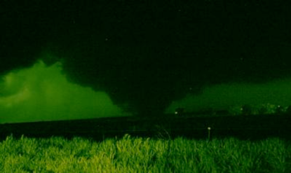
Figure 1: The Greensburg, KS Tornado. Greensburg, KS was destroyed on 4 May 2007. Photo by Van DeWald, NWS. From www.hprcc.unl.edu/nebraska/may4-2007Greensburg-Kansas-tornado.html.

A characteristic of models of the atmosphere is extreme sensitivity to small perturbations of the IC. This sensitivity, coupled with the uncertainty inherent in models and observations, leads to a loss of predictability. Consequently, it is possible that a small change in the IC could produce a very different forecast. That is, a forecast of a very large specific impact on people, property, or nature might result from a particular (small, plausible) IC perturbation, i.e., one that is consistent with the uncertainties present. It turns out that it is possible, using a technique called 4d-VAR described below, to calculate the IC perturbation to produce a particular result. For example, suppose we calculate the perturbations to maximize the potential for tornadogensis. Then, if the calculated IC perturbations are small compared to the IC uncertainty, we must not discount the possibility of tornadoes forming even if the original (i.e., unperturbed) forecast did not indicate this possibility. Henderson et al. (2005) call this approach “exigent” forecasting because of the requirement of precision in the forecast and urgency in the response. In this paper we describe the potential application of exigent forecasting (XF) to forecasting severe weather precursors for tornadoes (Sect. 4). Because of current limitations for forecasting very small scales, such as severe storms and tornadoes, applications of XF must first focus on larger scales, such as the strength or path of a TC, or on the precursors to the small-scale high impact phenomena. In previous work we applied a slight variation of the XF approach to controlling TCs and a summary of that work is provided to demonstrate that XF works (Sect. 3).

Our implementation of XF is based on 4d-VAR (four-dimensional variational data assimilation). 4d-VAR is designed to adjust the IC of a numerical weather prediction model consistent with the uncertainty of the prior estimate of the IC while at the same time minimizing the misfit to available observations. For XF, the same approach is taken but instead of (or in addition to) fitting observations, a measure of damage, loss, or an equivalent proxy is maximized or minimized (Sect. 2). For example, XF of maximized significant tornado parameter (STP, Sect. 4.a) should be able to provide relative probabilities of the threat of tornadogenesis as a function of time and place. To accomplish this, a specialized cost function for 4d-VAR is needed. This cost function is designed to measure the likelihood and severity of tornado outbreaks, based on the synoptic and mesoscale conditions conducive to their formation—the cost function does not measure tornado damage directly. That is, we use the STP as a proxy that captures the key environmental controls of tornadic development. When 4d-VAR solves the XF problem a by-product will be the value of the background cost function that provides a measure of the likelihood of occurrence of the forecast exigent conditions, and the value of the STP cost function that provides an estimate of the likelihood of tornadogenesis. XF could be a useful complement to ensemble forecasting because the ensemble is designed to capture the overall distribution of future outcomes, but not necessarily the particular event of consequence that is the focus of XF.

In the future, XF is expected to have very significant potential for societal benefits and to be applicable to a wide array of problems (Sect. 5). We note that operational forecasting of severe high-impact weather and subsequent decision-making is extremely time-sensitive. We comment on efficient implementation briefly in Sect. 4.c. XF has the potential to provide specific guidance of worst case results to focus the forecast and decision-making activity. The study of XF is expected to advance knowledge of forecasting high impact weather events and to result in refined methodologies for communicating warning and potential impacts of exigent weather events on a threatened population. XF might be extended to commercially viable products, such as forecasting freezes for the citrus industry. In addition, XF could be extended to deal with parametric uncertainty (e.g., the uncertain knowledge of the surface roughness height, $z_{0}$). Finally, XF should prove to be a useful device for laboratory exercises at the university level.

2 4d-VAR methodology

For operational weather forecasting, 4d-VAR finds the smallest increment at the start of each data assimilation period so that the perturbed nonlinear solution best fits all the available data. Mathematically, 4d-VAR blends background (i.e., a short-term forecast) and observations by minimizing a functional,

$$J=\mbox{$J_{b}$}+\mbox{$J_{o}$},$$ (1)

with respect to a control vector $\mathbf{{x}}$ that describes the atmospheric state. Here $J_{b}$ and $J_{o}$ measure the misfit of the four-dimensional analysis (i.e., the simulation that begins with $\mathbf{{x}}$) to the background and observations, respectively. 4d-VAR solves this complex nonlinear minimization problem iteratively, making use of the linear adjoint of the model, linearized about the current nonlinear simulation. Note that $J_{b}$ is defined by specifying the forecast error covariance—an unresolved problem for the storm-scale as well as for TCs and other severe weather. For exploratory experiments, available climatological background error covariances appropriate for mesoscale forecasts of similar resolution and for similar synoptic regimes could be used. A hybrid ensemble/4d-VAR would provide improved covariances (Sect. 5.a).

4d-VAR and XF are useful and indeed possible because the atmosphere is chaotic and unpredictable. Atmospheric motions occur over a huge spectrum of scales ranging from the jet stream to the trajectory of a cloud drop. Errors at different scales are coupled by nonlinear interactions. Tiny errors inevitably present in the large scales very quickly result in errors in the position of small-scale features. At the same time, errors present in small scales grow quickly and soon become unpredictable. These errors then effect somewhat larger scales and so on. The net effect is that very small perturbations can grow quickly. 4d-VAR finds perturbations that grow in just the correct way to best fit the available data or to best satisfy the XF constraints.

A few changes must be made to 4d-VAR for XF (Henderson et al. 2005): the control vector remains $\mathbf{{x}}$, $J_{b}$ is unchanged, $J_{o}$ may be present or not depending on whether more recent observations are available, and $J_{d}$ (“d” for “damage”) is added to measure the “benefits” minus “costs” resulting from the forecast as defined by the customer. The functional to be minimized for XF is then

$$J=\mbox{$J_{b}$}+\mbox{$J_{o}$}+w_{d}\mbox{$J_{d}$}.$$ (2)

The definition of $J_{d}$ should be nondimensional and $w_{d}$ is an adjustable weight. As $w_{d}$ is increased, the value of $J_{d}$ determined will decrease and vice versa. Note that $J_{d}$ is defined to calculate a worst case scenario: minimizing $J$ will simultaneously maximize costs, minimize benefits, and minimize increments with respect to the background and observations. By contrast, in our hurricane modification experiments (Sect. 3), by defining $J_{d}$ to measure damage alone, our solutions must minimize damage. That is, we calculated a “best case scenario” to determine perturbations to reduce damage.

In 4d-VAR data assimilation, the final value of $J_{b}+J_{o}$ objectively quantifies the likelihood of the calculated changes to $\mathbf{{x}}$, based on the most recent background, the observations, and knowledge of instrument and model error. This is the case since the log of the probability of an atmospheric state, given the background, the observations, and the associated uncertainties, is directly related to $J_{b}+J_{o}$ according to Bayes’ theorem when suitable assumptions are valid (Lorenc 1986). Note that smaller values of $J$ indicate higher probability. Since this applies to any atmospheric state, the final value of $J_{b}$ in the XF case will still be related to the likelihood of the exigent solution occuring. It is expected that $J$ has a $\chi^{2}$-distribution (Desroziers and Ivanov 2001; Muccino et al. 2004). In the XF situation, the final value of $J_{b}$ will still be related to the likelihood of the exigent solution occuring. As described in the next paragraph, by calculating the final value of $J_{b}$ as a function of the region used in the definition of $J_{d}$, we will obtain a map of the relative probability of the exigent event (e.g., of the occurrence of tornadogenesis).

Ideally the objective evaluation would be combined with a subjective evaluation based on forecaster experience—including pattern matching—that would compare the new analysis and observations to determine if the perturbation is consistent with hypothetical, but plausible, dynamical processes or additional observations. A series of solutions with increasing $w_{d}$, the weight given to $J_{d}$, gives a series of solutions that are increasingly unlikely (i.e., larger $J_{b}$) and associated with increasing (tornado) threat. One would stop increasing $w_{d}$ when the subjective evaluation indicates a nonrealistic solution or when the calculated likelihood becomes smaller than a prespecified lower value. Plotting the values, respectively, of $J_{d}$ and $J_{b}$ at the minimizing solution, with respect to $w_{d}$ for each location and forecast time, will allow us to highlight the locations and times of greatest threat.

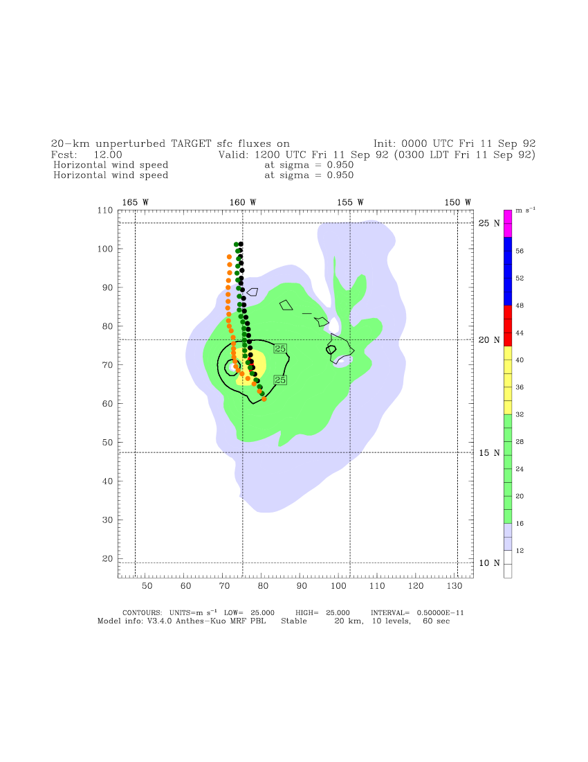
Figure 2: Forecast tracks of Hurricane Iniki. The center of the simulated hurricane is plotted for each hour for $\mathrm{{{t_{0}=0}}\mbox{{~{}}}{h}}$ to $\mathrm{{{24}}\mbox{{~{}}}{h}}$ for the unperturbed simulation (black dots) and for two target experiments, one allowing perturbations to all variables (orange) and one allowing only temperature perturbations (green). For reference, these tracks are plotted over the wind speeds of the repositioned cyclone used as the goal. Wind speeds corresponding to different Saffir-Simpson categories are plotted with different colors: grey for tropical depressions ($\mathrm{{{>12}}\mbox{{~{}}}{m\;s^{-1}}}$), green for tropical storms ($\mathrm{{{>17}}\mbox{{~{}}}{m\;s^{-1}}}$), yellow for category 1 hurricanes ($\mathrm{{{>33}}\mbox{{~{}}}{m\;s^{-1}}}$) and red for category 2 hurricanes ($\mathrm{{{>43}}\mbox{{~{}}}{m\;s^{-1}}}$). After Hoffman et al. (2006b).

3 An XF prototype: Weather control for hurricanes

Experiments we conducted demonstrate the ability of 4d-VAR to calculate the influence of perturbation on the future path or intensity of a simulated TC. In “target” experiments, the MM5 4d-VAR system determines the optimal atmospheric state trajectory, which simultaneously minimizes the size of the initial perturbation and the difference (using a quadratic norm) between the new forecast state and a goal atmospheric state in which the simulated cyclone has been repositioned. That is, $J_{d}$ in these experiments is similar in form to $J_{b}$, but instead of measuring the difference between the analysis and the background, $J_{d}$ here measures the difference between a short (in the case presented later six-hour) forecast and the goal or target. In experiments for Hurricane Iniki, the simulated hurricane successfully matched the goal state at the end of the 4d-VAR period, then continued on a track parallel to its original track, and missed the Island of Kauai as desired (Hoffman et al. 2006b). Perturbations to the initial conditions are small relative to the hurricane. When changes are restricted to the temperature field alone, the technique is less successful (Fig. 2).

In “damage cost function” experiments, 4d-VAR simultaneously minimized the size of the initial perturbation and an estimate of property loss that depends on wind speed. In these experiments $J_{d}$ is given by

$$J_{d}=\frac{1}{\Delta t}\frac{1}{A}\int\limits_{\Delta t}\int\limits_{A}D(x,y,t)P(x,y),$$ (3)

where $\Delta t$ is the time period of interest and $A$ is the area of interest. The fractional wind damage $D$ is taken to depend only on the lowest model layer wind speed at location $(x,y)$ with the functional form shown in Fig. 3, and the property values $P(x,y)$ were assigned based on a land use data base. (Details are given by Henderson et al. (2005).)

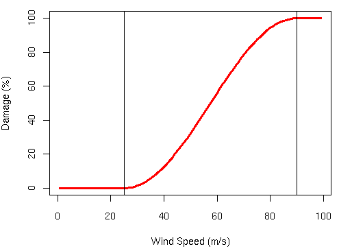
Figure 3: Wind cost function. In our model of wind damage, wind speeds less than $\mathrm{{{25}}\mbox{{~{}}}{m\;s^{-1}}}$ cause no damage and wind speeds in excess of $\mathrm{{{90}}\mbox{{~{}}}{m\;s^{-1}}}$ cause total loss. Between these two threshold wind speeds a cosine curve parameterizes the percent of wind damage.

In experiments for Hurricane Andrew, the hurricane surface winds decrease over the built-up area at landfall (Henderson et al. 2005). Additional experiments explored the ability of other state variables to effect desired changes to Hurricane Iniki. Perturbations restricted to winds alone, to temperature alone, or even to temperature only outside the center of the hurricane were found to be effective (Hoffman et al. 2006a). Furthermore, vertical velocity and humidity perturbations alone were ineffective at reducing damaging winds. An experiment using perturbation pressure alone substantially reduced the extent of damaging winds. While this result is similar to experiments that used solely temperature in the control vector, the minimization failed to converge to within specified numerical limits and thus should be considered less robust.

The optimal perturbations usually include quasi-axisymmetric features centered on the hurricane (Fig. 4). It appears that the perturbations then evolve as concentric wave disturbances that propagate to a focus at the hurricane center, and convert the kinetic energy of the hurricane into thermal potential energy at the appropriate time. The hurricane surface winds regenerate soon thereafter, so a continuous series of perturbations may be needed in practice (Fig. 5).

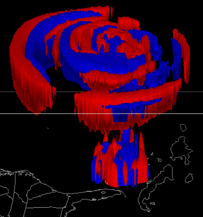
Figure 4: Initial perturbation for Hurricane Andrew. In this color volume rendering of optimal initial temperature perturbations for Hurricane Andrew, the red and blue surfaces enclose the volumes where the perturbations are greater than $\mathrm{{{0.6}}\mbox{{\mbox{${{~{}}}^{\circ}$}}}{C}}$, and less than $\mathrm{{{-0.6}}\mbox{{\mbox{${{~{}}}^{\circ}$}}}{C}}$, respectively.

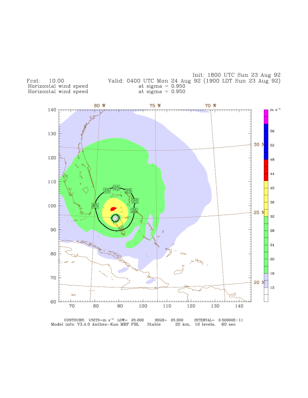
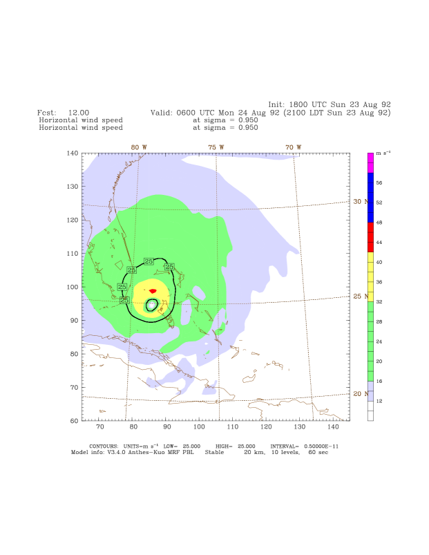
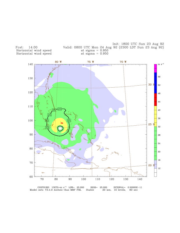
4 h 6 h 8 h Unperturbed Controlled

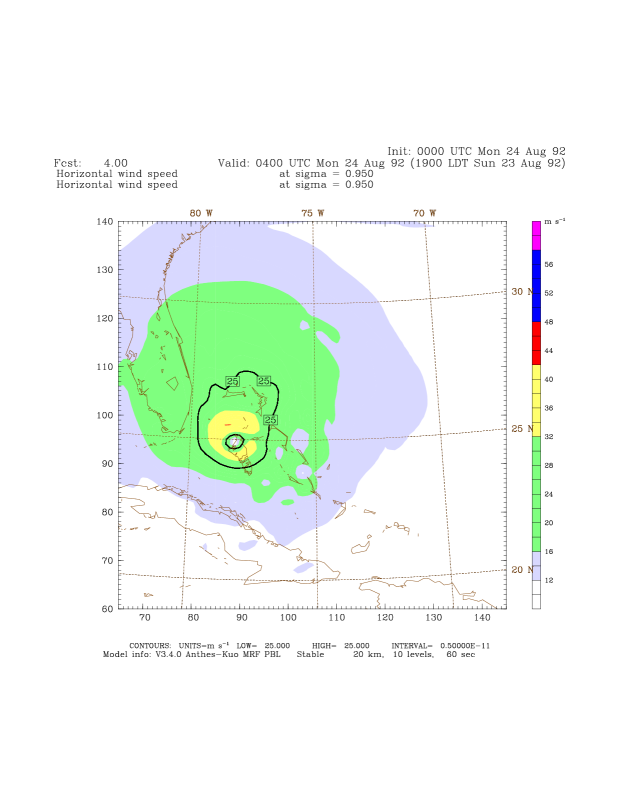
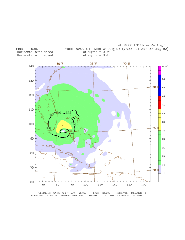
Figure 5: Hurricane Andrew surface wind fields. Evolution of the surface wind field for the unperturbed simulation and for the controlled experiment that minimized damage between 4 and $\mathrm{{{6}}\mbox{{~{}}}{h}}$ by introducing temperature perturbations only. Wind speed is color coded according to the Saffir-Simpson scale (as in Fig. 2) and the damaging wind contour $\mathrm{{{25}}\mbox{{~{}}}{m\;s^{-1}}}$ is plotted at 4, 6, and $\mathrm{{{8}}\mbox{{~{}}}{h}}$ after the perturbation is introduced. In the experiments only wind speeds above $\mathrm{{{25}}\mbox{{~{}}}{m\;s^{-1}}}$ result in property damage. Note that at $\mathrm{{{6}}\mbox{{~{}}}{h}}$ there are no damaging winds over land areas in the controlled experiment. After Henderson et al. (2005).

4 Application to tornadogenesis precursors

A combination of inaccuracy in the initial conditions (IC), model errors, and the short predictability time scale for severe storms all combine to make tornado forecasting very difficult. Especially challenging are parameterizing the moist microphysics and estimating the IC for water vapor, cloud, and precipitation since in stormy environments these have small spatial scales (e.g., Weiss et al. 2007). As a result, prediction of severe weather generally uses an ingredients-based forecast method wherein coincidence of multiple individual atmospheric predictors increases forecaster confidence in the likelihood of severe weather. Historically, the risk of severe weather is maximized when and where the ingredients coincide. The discussion here will focus on one aspect of this overall problem—the IC uncertainty for dry-line tornadogenesis, where the empirical ingredients-based approaches work best. The XF approach has greater applicability than this one focus. In other parts of this paper, we sketch the extensions needed to handle directly forecasting storm scale high impact weather elements as well as other high impact or high value weather events such as landfalling hurricanes and freezing conditions in citrus growing regions.

Ingredients-based indices, due to their nature, tend to focus on prediction of sensible weather conditions, such as the likelihood of supercell thunderstorms or significant tornadoes, whereas individual indices or ingredients describe more esoteric atmospheric features, such as the magnitude of thermal instability.

a Cost function for dryline tornadogenesis

XF of tornadogenesis based on 4d-VAR requires a cost function based on an ingredients-based index. One ingredients-based index that can define $J_{d}$ is the significant tornado parameter (hereafter, STP). The STP combines individual measures of atmospheric thermal stability, boundary layer moisture and horizontal wind fields. This index has been shown subjectively to discriminate between convective events involving discrete supercells that produce significant tornadoes and those that produce weak tornadoes or none at all. The requirement that the mode of the expected convection be discrete supercells limits the applicability of STP-based XF. In other situations, other more appropriate indices should be used.

As defined by Thompson et al. (2003),

STP $$= \frac{\mbox{MLCAPE}}{\mbox{$\mathrm{{1000}\mbox{{~{}}}{J\;kg^{-1}}}$}}\>\times\>\frac{\mbox{SHR}}{\mbox{$\mathrm{{{20}}\mbox{{~{}}}{m\;s^{-1}}}$}}$$ (4)

$$\times \frac{\mbox{SRH}}{\mbox{$\mathrm{{100}\mbox{{~{}}}{m^{2}\;s^{-2}}}$}}\>\times\>\frac{2000-\mbox{MLLCL}}{\mbox{$\mathrm{{1500}\mbox{{~{}}}{m}}$}}$$

$$\times \frac{150-\mbox{MLCIN}}{\mbox{$\mathrm{{125}\mbox{{~{}}}{J\;kg^{-1}}}$}},$$

where MLCAPE is the mixed-layer convective available potential energy (CAPE), SHR is the magnitude of the 0-6 km vertical shear of the horizontal wind, SRH is the magnitude of the 0-1 km storm relative helicity, MLLCL is the mixed-layer lifted condensation level (LCL), and MLCIN is the mixed-layer convective inhibition (CIN). Values of STP greater than one are associated with the potential for significant tornadoes. Each of the components of STP has a history of use in tornado prediction and each describes characteristics of the local storm environment as detailed in Table 1. We believe that use of the STP as a penalty function may be especially relevant to characterizing the likelihood of CIN erosion—a frequent forecasting problem and one that strongly modulates the overall extent of convection. The definition of STP is empirical and continues to be refined by Thompson et al. (2004, 2007). However, for a preliminary study the definition given in Eq. (4) should be adequate. A straightforward approach to defining $J_{d}$ so that minimizing $J$ defined in Eq. (2) will result in maximizing the STP is to average STP over a target area $A$, and time interval $\Delta t$:

$$J_{d}=-\frac{1}{\Delta t}\frac{1}{A}\int\limits_{\Delta t}\int\limits_{A}\mbox{STP}.$$ (5)

Typically $A$ will be a county of interest, and $\Delta t$ a period of interest lasting from one to several hours.

Table 1: STP ingredients

CAPE	CAPE is a measure of the instability through the depth of the atmosphere, i.e., the positive buoyant energy available, and is generally proportional to the updraft strength of a storm. Values of CAPE over $\mathrm{{4000}\mbox{{~{}}}{kg^{-1}}}$ indicate extreme instability likely associated with high lapse rates.
SHR	The magnitude of the deep-layer wind shear, along with the amount of instability, regulates the overall dynamical organization and persistence of a storm. Values of wind shear greater than $\mathrm{{{20}}\mbox{{~{}}}{m\;s^{-1}}}$ in NCEP Rapid Update Cycle Version 2 model soundings have been shown by Thompson et al. (2003) to strongly support development of supercells.
SRH	The storm-relative helicity is a measure of the potential of low-level cyclonic updraft rotation for right-moving supercells, i.e., supercells that move slightly to the right of the mean flow for a cyclonically curved hodograph. Values over $\mathrm{{100}\mbox{{~{}}}{m^{2}\;s^{-2}}}$ are often seen with tornadic supercells. Weisman and Rotunno (2000) describe how wind shear and helicity determine supercell dynamics.
MLLCL	Lower values of environmental LCL, related to high mixed-layer relative humidities, tend to increase the potential buoyancy of rear flank downdrafts in storms capable of supporting significant tornadoes (Markowski et al. 2003).
CIN	CIN is a measure of the work required to lift air to its level of free convection. It represents the “negative” area on a sounding and is often likened to a physical “cap” to explosive thunderstorm development. A number of atmospheric processes can erode this negative area, including synoptic scale upward motion, upward motion along a boundary and surface heating. Values of CIN associated with convection later in the day are often greater (closer to zero) than -$\mathrm{{250}\mbox{{~{}}}{J\;kg^{-1}}}$. This term strongly regulates the spatial extent of significant STP.

As defined by Eq. (5), $J_{d}$ is a highly nonlinear function of the atmospheric state vector, since not only is it a product of the five separate terms in Eq. (4), but the individual terms themselves are highly nonlinear: CAPE and CIN correspond to the areas between a lifted parcel and the environmental sounding on a thermodynamic diagram, and are highly sensitive to changes in the mixed layer quantities that define the parcel. Similarly, the storm-relative helicity depends on an estimate of storm motion, which in turn depends on the depth of the convectively unstable layer. Formally, the nonlinearities in $J_{d}$ can be treated in the same way 4d-VAR handles nonlinearities in model parameterizations and in complex observation operators. In the framework of iterative 4d-VAR, the full nonlinear formulation is used in the outer loop, and linearized formulations (forward and adjoint) are used in the inner loop (Lorenc 1997; Rabier et al. 2000). However, strong nonlinearities, such as “on-off” switches from stable to unstable conditions, can lead to convergence problems during the minimization. Therefore, to enhance the performance of 4d-VAR, some or all of the individual terms of STP should be modified. The modified versions will be better behaved in terms of being differentiable and less nonlinear. A general approach is to smooth out non-differentiable points. Note that since STP has been defined and refined empirically, relatively small changes to the formulation of STP should be acceptable for current purposes.

b Key dryline tornadogenesis cases

For demonstration, the 4d-VAR XF method should be applied to Major Tornado Outbreak Days (Schneider et al. 2004), which have historically accounted for nearly 50% of all fatalities. These are calendar days during which there are at least six significant tornadoes, i.e., F2 and higher rating on the Fujita scale (Fujita 1971). (It should be noted that the Fujita scale is used here and not the newer (February 2007) Enhanced Fujita Scale.) Typically, Major Tornado Outbreak Days exhibit robust signatures for tornadogenesis in soundings and NWP fields and are identified by SPC forecasts as having a “moderate” or “high” risk for severe weather. Furthermore, initial case studies should be focused on afternoon-evening springtime convective events in the form of discrete supercells. These conditions often are met near the dryline in the Central and Southern Plains of the United States. Finally, because small-scale boundaries in the domain caused by previous convection (outflow boundaries, etc.) will not be well represented by a model with currently available resolution and parameterizations, only events which are substantially separate, in space and time, from earlier convection should be considered. Candidate demonstration cases are listed in Table 2. The characteristics of the 1985 outbreak make it the archetypical example for our purposes.

Table 2: Examples of dryline tornadogenesis

31 May 1985	41 tornadoes, centered in NW Pennsylvania and north of Toronto, Ontario, formed ahead of a cold front during the afternoon and evening hours, killing 88 people. The only F5 tornado in Pennsylvania history destroyed the town of Wheatland. Forbes (1985) and Ferguson et al. (1986) have documented the statistics of the outbreak, while Farrell and Carlson (1989) attributed an elevated mixed layer (EML) as being a major factor in the generation of the large latent instability available to the convection. EMLs (Lanicci and Warner 1991) are frequently associated with convective outbreaks in the Plains of the US, yet rarely are displaced this far to the northeast. This case appears to be an excellent case to study due to its overall robust and spatially distinct synoptic characteristics, predominant supercellular mode of convection, and the removal of the “cap” below the EML, i.e., there is no CIN below the EML.
3 May 1999	This outbreak of 66 tornadoes in Oklahoma and Kansas highlighted the risk to densely populated urban areas when an F5 tornado passed through Moore, OK, a suburb of Oklahoma City. A total of 46 people were killed by the outbreak. Roebber et al. (2002) and Edwards et al. (2002) describe the subtleties in the synoptic and mesocale environment of the outbreak which lowered confidence in many aspects of the forecasting of this outbreak.
4-5 May 2007	4-5 May 2007 - On back-to-back days there were major tornado outbreaks in the Plains, including the first EF5-rated tornado which destroyed Greensburg, KS (McCarthy et al. 2007). Synoptic conditions were conducive to supercellular storms during both afternoons and evenings in approximately the same geographical area. On the 4th, great instability was present, but weak convergence along the dryline, weak forcing aloft, and a capping inversion combined to limit the number of storms that formed, especially farther south (Weiss et al. 2007).

c Mode of operation and validation

For demonstration purposes we would apply this procedure to a few cases selected for study. For the historical cases we can examine $J_{d}$ for times and locations surrounding the actual tornadoes that did occur. For validation we will then subjectively compare the maps of $J_{d}$ to the tornado reports. We anticipate that high values of $J_{d}$ will be correlated with the occurrence and intensities of observed tornadoes. Such a finding will be necessary to consider the method useful. While forecasts of severe storms are expected to be improved with the most sophisticated physical parameterizations and the highest possible resolution, for forecasting precursor situations predominantly forced by synoptic scale advection, the forecast model requirements are much less stringent. A typical 4d-VAR setup would use the Weather Research and Forecast (WRF) model configured with the YSU (Yonsei University) PBL parameterization (Hong et al. 2006) and the Anthes Kuo convection scheme, a single-moment microphysics scheme with multiple liquid and ice water species, and the RRTM radiation package. The initial and boundary conditions for 4d-VAR case studies are available eight-times daily at $\mathrm{{{32}}\mbox{{-}}{km}}$ resolution from the North American Regional Reanalysis Project (Mesinger et al. 2006).

Calculating the worst case for different areas and times will provide a measure of threat. Skilled on-duty forecasters now issue outlooks for medium- and high-risk convective situations one to three days in advance. Alternatively, the Short Range Ensemble Forecast (SREF) system can be used to identify times and areas with non-zero probability of values of STP exceeding a critical threshold (Bright et al. 2008). In either case, detailed exigent forecasts would be made 3–12 hours in advance for the areas and times at risk. Typically, in Eq. (5) the area $A$ will be a county, the time interval $\Delta t$ will be one hour centered on a desired forecast time, and $J$ defined in Eq. (2) will be minimized for all areas and time intervals that are considered at risk or are in the neighborhood of areas and time intervals at risk. This will produce a sequence of maps of $J_{d}$ (at constant $J_{b}$ as described in Sect. 2) that we anticipate will prove very useful to the operational forecaster.

The methodology described here (and in Sect. 2) may be quite computer intensive, yet operations in a “warn on forecast” setting are quite time sensitive. There are probably many possible approaches to increase efficiency. First, 4d-VAR can find the minimum faster if it starts with a good estimate. Having found the minimum for one location and time, that solution may prove to be useful for starting the search for neighboring locations and times. Second, resources should be concentrated on locations and times most at risk. For example if we first minimize $J$ for a large region $A$ and long time interval $\Delta t$, then we should be able to identify, in that minimizing solution, smaller regions and time intervals most at risk (i.e., where STP is large) for further analysis. And this process would then be iterated down to the smallest scales required, but just at the most critical locations and times.

5 Future context and outlook

In this paper we discussed XF of the precursors of tornadoes in an attempt to avoid missed forecasts. We identified dry-line tornadogenesis precursors as a relevant but doable high impact weather phenomena. The concept of XF is new and can be extended in many ways. In the future, with further developments of WFR 4d-VAR, new classes of XF experiments will become possible (Sect. 5.a). Additional potential applications are briefly described in Sect. 5.b.

a Beyond precursors

XF may benefit operational forecasters by identifying minor changes to model initial conditions that would strongly influence the weather in their forecast regions. Also, this technique might help to identify model or analysis system deficiencies when applied to poorly predicted historical cases. The sensitivity of severe storms or hurricanes to slight changes in environmental flow, their complex dynamics, their relatively compact size, and their impact on lives and property make them interesting candidates for study from the XF perspective. But many other situations could be usefully examined this way. Examples include local extreme weather events, such as heavy precipitation, strong winds and extreme temperatures, as well as situations in which a non-linear response in societal or economic costs results from modest changes to seemingly innocuous values of the meteorological variables, such as a reduction in surface temperatures to slightly below freezing in a region of citrus production. XF is applicable when the consequences of a weather event, be they financial, related to human safety, or otherwise, would be significant whether or not the meteorological situation is considered “significant”. Ultimately the technique involves evaluating the reasonableness of calculated changes to the existing analysis obtained by presenting 4d-VAR with the usual model background field, observations, and a cost function term related to the specific event of consequence.

Despite these promising opportunities, a number of limitations now combine to constrain the experiments that could be conducted. The critical limitations are the initial conditions, models, background cost function, and impact of nonlinearities. Because of these limitations we have described a potential demonstration project to forecast precursor situations predominantly forced by synoptic scale advection. The outlook for overcoming these limitations is reviewed here.

Initial conditions: Spinning up a realistic severe storm simulation is fraught with difficulty. The use of high resolution radar and satellite data to properly initialize a mesoscale model is an area of ongoing research. The success of the technique in application to actual exigent weather phenomena as opposed to precursors of such phenomena will require greatly improved capability to initialize the relevant structures in NWP models.

Model errors: As described above, the effect of model errors is not accounted for by XF. Including additional elements in the control vector can allow for the possibility of model error. For example, following the idea of Trémolet (2005), perturbations can be introduced at intervals within the 4d-VAR interval. Also see Sect. 5.b.ii below.

Background cost function: Available background error covariances may not be appropriate for the particular synoptic situations of interest. For background error covariances, XF can make use of an ensemble of forecasts, such as from a short-range ensemble forecast (SREF) system (e.g., Grimit and Mass 2002).

Nonlinearities: Incremental or not, 4d-VAR relies on linearizing the governing equations, and on the adjoint of the tangent linear model. This results in some difficulties. First, having the correctly coded adjoint is not a guarantee of success. For example, linear instabilities can sometimes be present in the tangent linear and adjoint versions while the corresponding nonlinear parameterization is well behaved (Mahfouf 1999). That is, a formally correct adjoint model can be computationally unstable. Furthermore, such an instability may only be apparent in a stressing situation, e.g., a cloud resolving severe storm simulation or a high resolution hurricane simulation. Second, even at short forecast times, linearization errors can be large (Trémolet 2004). In principle the brute force approach can be used. It now appears that sufficient computational power has become available to apply this approach to research questions in a case study context using a detailed mesoscale model (Martin and Xue 2004).

b Further applications

i Forecast sensitivity studies

Variants of XF 4d-VAR have been used to examine forecast sensitivity. Singular vectors are commonly used to identify forecast sensitivity (e.g., Gelaro et al. 1998). This is normally a linear sensitivity in which the moist processes are often simplified or neglected, although some authors (e.g., Reynolds and Rosmond 2003) have examined how singular vectors evolve nonlinearly once they are determined. The choice of the norm that measures the size of the singular vector at the end of the evolution period is analogous to our $J_{d}$. For example, singular vectors can be targeted to particular regions (e.g., Puri et al. 2001). To do so, the amplification during the forecast of a small initial perturbation is maximized with respect some norm, such as kinetic energy within a particular region. The singular vector pattern in the initial conditions may then be used to design a targetted observing strategy.

XF may be considered to be a nonlinear form of singular vector analysis. XF might provide further refinement in any study or application that makes use of singular vectors. For example the XF approach could be used to diagnose how and why a critical forecast failed. For this purpose $J_{d}$ would measure the difference between forecast and key elements of what in fact happened. The control vector could be restricted to small regions or just a subset of the prognostic variables to establish what part of the initial conditions were to blame for the poor forecast. Recent work along these lines is reported by Rivière et al. (2008) and Mu et al. (2009).

ii Parameter sensitivity

The existing MM5 and WRF 4d-VAR systems are geared towards data assimilation, and the control vector used in the optimization process contains just the variables defining the initial state of the model. It is also of interest to consider the sensitivity to other parts of the modeling system considered constant during the data assimilation process. For example, tunable parameters of physics packages, or “fixed” external data such as the roughness length ($z_{0}$) or the antecedent soil moisture, are not known exactly, and could thus also be included in the control vector and adjusted alongside the initial conditions. Such approaches have been used in oceanic (e.g., Smedstad and O’Brien 1991; Sheinbaum 1995) and atmospheric (e.g., Wang et al. 2005; Norris and da Silva 2007) data analysis and assimilation. Within XF, this would address the possibility that plausible changes in model parameters could, at least in part, lead to a model solution that maximizes tornado genesis potential. The associated changes to the software would be isolated to two separate parts of the 4d-VAR system: transformations from the control vector used in the optimization to model state variables and parameters, and the physical packages affected by the tunable parameters or external data under consideration.

iii Teaching tool

There are many potential uses of the WRF system for teaching undergraduate and graduate meteorology. The XF approach allows one to pose “what-if” lab exercises. For example, what is the minimum and maximum QPF to be expected from a particular synoptic situation given the uncertainty in IC? Or how much would SST have to be reduced to change a category 4 hurricane into a category 3 hurricane?

References

- Bright et al. (2008) Bright, D., S. Weiss, R. Schneider, G. Grosshans, and J. Levit, 2008: SPC ensemble applications: Current status, recent developments, and future plans. 4th NCEP/NWS Ensemble User Workshop, Laurel, MD.
- Desroziers and Ivanov (2001) Desroziers, G. and S. Ivanov, 2001: Diagnosis and adaptive tuning of observation-error parameters in a variational assimilation. Quart. J. Roy. Meteor. Soc., 127 (574), 1433–1452.
- Edwards et al. (2002) Edwards, R., S. F. Corfidi, R. L. Thompson, J. S. Evans, J. P. Craven, J. P. Racy, D. W. McCarthy, and M. D. Vescio, 2002: Storm Prediction Center forecasting issues related to the 3 May 1999 tornado outbreak. Wea. Forecasting, 17 (3), 544–558.
- Farrell and Carlson (1989) Farrell, R. J. and T. N. Carlson, 1989: Evidence for the role of the lid and underunning in an outbreak of tornadic thunderstorms. Mon. Wea. Rev., 117 (4), 857–871.
- Ferguson et al. (1986) Ferguson, E. W., E. P. Ostby, and P. W. Leftwich, Jr., 1986: 1985 – An average year for tornadoes. Weatherwise, 39, 33–39.
- Forbes (1985) Forbes, G. S., 1985: Preliminary tornado statistics – May 31, 1985 outbreak. Weatherwise, 38, 194–195.
- Fujita (1971) Fujita, T. T., 1971: Proposed characterization of tornadoes and hurricanes by area and intensity. SMRP Research Paper 91, University of Chicago, available from Wind Engineering Research Center, Texas Tech University, P.O. Box 41023, Lubbock, TX 79409-1023.
- Gelaro et al. (1998) Gelaro, R., R. Buizza, T. N. Palmer, and E. Klinker, 1998: Sensitivity analysis of forecast errors and the construction of optimal perturbations using singular vectors. J. Atmos. Sci., 55 (6), 1012–1037.
- Grimit and Mass (2002) Grimit, E. P. and C. F. Mass, 2002: Initial results of a mesoscale short-range ensemble forecasting system over the Pacific Northwest. Wea. Forecasting, 17, 70–83.
- Henderson et al. (2005) Henderson, J. M., R. N. Hoffman, S. M. Leidner, T. Nehrkorn, and C. Grassotti, 2005: A 4D-VAR study on the potential of weather control and exigent weather forecasting. Quart. J. Roy. Meteor. Soc., 131, 3037–3052.
- Hoffman et al. (2006a) Hoffman, R. N., J. M. Henderson, S. M. Leidner, C. Grassotti, and T. Nehrkorn, 2006a: The response of damaging winds of a simulated tropical cyclone to finite amplitude perturbations of different variables. J. Atmos. Sci., 63 (7), 1924–1937.
- Hoffman et al. (2006b) ———, 2006b: Using 4d-VAR to move a simulated tropical cyclone in a mesoscale model. Computers and Mathematics with Applications, 52 (8-9), 1193–1204.
- Hong et al. (2006) Hong, S.-Y., Y. Noh, and J. Dudhia, 2006: A new vertical diffusion package with an explicit treatment of entrainment processes. Mon. Wea. Rev., 134 (9), 2318–2341.
- Lanicci and Warner (1991) Lanicci, J. M. and T. T. Warner, 1991: A synoptic climatology of the elevated mixed-layer inversion over the Southern Great Plains in spring. Part III: Relationship to severe-storms climatology. Wea. Forecasting, 6, 214–226.
- Lorenc (1986) Lorenc, A. C., 1986: Analysis methods for numerical weather prediction. Quart. J. Roy. Meteor. Soc., 112, 1177–1194.
- Lorenc (1997) ———, 1997: Development of an operational variational assimilation scheme. J. Meteor. Soc. Japan, 75 (1B), 339–346.
- Mahfouf (1999) Mahfouf, J.-F., 1999: Influence of physical processes on the tangent-linear approximation. Tellus A, 51 (2), 147–166.
- Markowski et al. (2003) Markowski, P. M., J. M. Straka, and E. N. Rasmussen, 2003: Tornadogenesis resulting from the transport of circulation by a downdraft: Idealized numerical simulations. J. Atmos. Sci., 60 (6), 795–823.
- Martin and Xue (2004) Martin, W. J. and M. Xue, 2004: Initial condition sensitivity analysis of a mesoscale forecast using very large ensembles. 20th Conference on Weather Analysis and Forecasting/16th Conference on Numerical Weather Prediction, American Meteorological Society, Boston, MA, Seattle, Washington, paper J8.2.
- McCarthy et al. (2007) McCarthy, D., L. Ruthi, and J. Hutton, 2007: The Greensburg, KS tornado. 22nd Conference on Weather Analysis and Forecasting/18th Conference on Numerical Weather Prediction, American Meteorological Society, Boston, MA, Park City, Utah, paper J2.4; http://ams.confex.com/ams/pdfpapers/126927.pdf.
- Mesinger et al. (2006) Mesinger, F., G. DiMego, E. Kalnay, K. Mitchell, P. C. Shafran, W. Ebisuzaki, D. Jovic̀, J. Woollen, E. Rogers, E. H. Berbery, M. B. Ek, Y. Fan, R. Grumbine, W. Higgins, H. Li, Y. Lin, G. Manikin, D. Parrish, and W. Shi, 2006: North American Regional Reanalysis. Bull. Amer. Meteor. Soc., 87 (3), 343–360.
- Mu et al. (2009) Mu, M., F. Zhou, and H. Wang, 2009: A method for identifying the sensitive areas in targeted observations for tropical cyclone prediction: Conditional nonlinear optimal perturbation. Mon. Wea. Rev., 137 (5), 1623–1639.
- Muccino et al. (2004) Muccino, J. C., N. F. Hubele, and A. F. Bennett, 2004: Significance testing for variational assimilation. Quart. J. Roy. Meteor. Soc., 130 (600), 1815–1838.
- Norris and da Silva (2007) Norris, P. M. and A. M. da Silva, 2007: Assimilation of satellite cloud data into the GMAO finite-volume data assimilation system using a parameter estimation method. Part I: Motivation and algorithm description. J. Atmos. Sci., 64 (11), 3880–3895.
- Puri et al. (2001) Puri, K., J. Barkmeijer, and T. N. Palmer, 2001: Ensemble prediction of tropcial cyclones using targeted diabatic singular vectors. Quart. J. Roy. Meteor. Soc., 127 (572), 709–731.
- Rabier et al. (2000) Rabier, F., H. Järvinen, E. Klinker, J.-F. Mahfouf, and A. Simmons, 2000: The ECMWF operational implementation of four-dimensional variational assimilation. I: Experimental results with simplified physics. Quart. J. Roy. Meteor. Soc., 126 (564), 1143–1170.
- Reynolds and Rosmond (2003) Reynolds, C. A. and T. E. Rosmond, 2003: Nonlinear growth of singular vector-based perturbations. Quart. J. Roy. Meteor. Soc., 129 (594), 3059–3078.
- Rivière et al. (2008) Rivière, O., G. Lapeyre, and O. Talagrand, 2008: Nonlinear generalization of singular vectors: Behavior in a baroclinic unstable flow. J. Atmos. Sci., 65 (6), 1896–1911.
- Roebber et al. (2002) Roebber, P. J., D. M. Schultz, and R. Romero, 2002: Synoptic regulation of the 3 May 1999 tornado outbreak. Wea. Forecasting, 17 (3), 399–429.
- Schneider et al. (2004) Schneider, R. S., H. E. Brooks, and J. T. Schaefer, 2004: Tornado outbreak days: An updated and expanded climatology (1875-2003). 22nd Conference on Severe Local Storms, American Meteorological Society, Boston, MA, Hyannis, MA, 1–11, paper 12.1. Available at http://ams.confex.com/ams/11aram22sls/techprogram/paper_81933.htm.
- Sheinbaum (1995) Sheinbaum, J., 1995: Variational assimilation of simulated acoustic tomography data and point observations: A comparative study. J. Geophys. Res., 100 (C10), 20 745–20 761.
- Smedstad and O’Brien (1991) Smedstad, O. M. and J. J. O’Brien, 1991: Variational data assimilation and parameter estimation in an equatorial Pacific Ocean model. Progress Oceanogr., 26, 179–241.
- Thompson et al. (2003) Thompson, R. L., R. Edwards, J. A. Hart, K. L. Elmore, and P. Markowski, 2003: Close proximity soundings within supercell environments obtained from the Rapid Update Cycle. Wea. Forecasting, 18 (6), 1243–1261.
- Thompson et al. (2004) Thompson, R. L., R. Edwards, and C. M. Mead, 2004: An update to the supercell composite and significant tornado parameters. 22nd Conference on Severe Local Storms, American Meteorological Society, Boston, MA, Hyannis, MA, p8.1, http://ams.confex.com/ams/pdfpapers/82100.pdf.
- Thompson et al. (2007) Thompson, R. L., C. M. Mead, and R. Edwards, 2007: Effective storm-relative helicity and bulk shear in supercell thunderstorm environments. Wea. Forecasting, 22, 102–115.
- Trémolet (2004) Trémolet, Y., 2004: Diagnostics of linear and incremental approximations in 4D-Var. Quart. J. Roy. Meteor. Soc., 130 (601), 2233–2251.
- Trémolet (2005) ———, 2005: Accounting for an imperfect model in 4d-var. Technical Memorandum 477, ECMWF, Reading, United Kindom.
- Wang et al. (2005) Wang, J., M. Mu, and Q. Zheng, 2005: Initial condition and parameter estimation in physical ‘on-off’ processes by variational data assimilation. Tellus A, 57 (5), 736–741.
- Weisman and Rotunno (2000) Weisman, M. L. and R. Rotunno, 2000: The use of vertical wind shear versus helicity in interpreting supercell dynamics. J. Atmos. Sci., 57 (9), 1452–1472.
- Weiss et al. (2007) Weiss, S. J., J. S. Kain, D. R. Bright, J. J. Levit, G. W. Carbin, M. E. Pyle, Z. I. Janjic, B. S. Ferrier, J. Du, M. L. Weisman, and M. Xue, 2007: The NOAA Hazardous Weather Testbed: Collaborative testing of ensemble and convection-allowing WRF models and subsequent transfer to operations at the Storm Prediction Center. 22nd Conference on Weather Analysis and Forecasting/18th Conference on Numerical Weather Prediction, American Meteorological Society, Boston, MA, Park City, Utah, paper 6B.4; http://ams.confex.com/ams/22WAF18NWP/techprogram/paper_124772.htm.