Interval graph limits

Abstract.

We work out the graph limit theory for dense interval graphs. The theory developed departs from the usual description of a graph limit as a symmetric function $W(x,y)$ on the unit square, with $x$ and $y$ uniform on the interval $(0,1)$. Instead, we fix a $W$ and change the underlying distribution of the coordinates $x$ and $y$. We find choices such that our limits are continuous. Connections to random interval graphs are given, including some examples. We also show a continuity result for the chromatic number and clique number of interval graphs. Some results on uniqueness of the limit description are given for general graph limits.

1. Introduction

A graph $G$ is an interval graph if there exists a collection of intervals $\{I_{i}\}_{i\in V(G)}$ such that there is an edge $ij\in E(G)$ if and only if $I_{i}\cap I_{j}\neq 0$, for all pairs $(i,j)\in V(G)^{2}$ with $i\neq j$.

Example 1.1.

Figure 1(a) shows published confidence intervals for the astronomical unit (roughly the length of the semi-major axis of the earth’s elliptical orbit about the sun). Figure 1(b) shows the corresponding interval graph (data from Youden [43]).

(a) Confidence Intervals

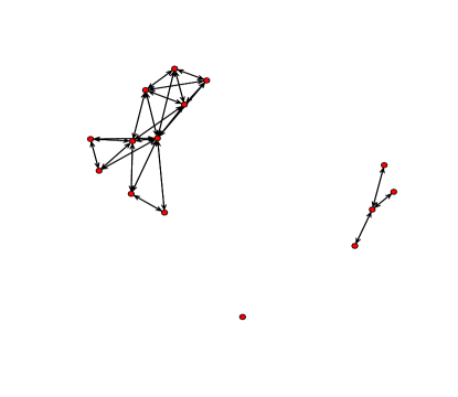
(b) Interval Graph

Figure 1. Building the interval graph for the Youden astronomical constant confidence intervals [43].

It is surprising how many missing edges there are in this graph as these correspond to disjoint confidence intervals for this basic unit of astronomy. Even in the large component, the biggest clique only has size $4$.

The literature on interval graphs and further examples are given in Section 2.1–2.3 below. Section 2.4 reviews the emerging literature on graph limits. Roughly, a sequence of graphs $G_{n}$ is said to converge if the proportion of edges, triangles and other small subgraphs tends to a limit. The limiting object is not usually a graph but is represented as a symmetric function $W(s,t)$ and a probability measure $\mu$ on a space ${\mathcal{S}}$. Again roughly $W(s,t)$ is the chance that the limiting graph has an edge from $s$ to $t$, more details will be provided in Section 2.4.

The main results in this paper combine these two sets of ideas and work out the graph limit theory for interval graphs. The intervals in the definition above may be arbitrary intervals of real numbers $[a,b]$, that without loss can be considered inside $[0,1]$. Thus an interval can be identified with a point in the triangle ${\mathcal{S}}:=\{[a,b]:0\leq a\leq b\leq 1\}$, see Figure 2. An interval graph $G_{n}$ is defined by a set of intervals $\{[a_{i},b_{i}]\}_{i=1}^{n}$, which may be identified with the empirical measure $\mu_{n}=\frac{1}{n}\sum\delta_{(a_{i},b_{i})}$. In Section 3 we show that a sequence of graphs $G_{n}$ converges if the empirical measures $\mu_{n}$ converge to a limiting probability $\mu$ in the usual weak star topology, provided $\mu$ satisfies a technical condition which we show may be assumed. The limit of the graphs is specified by a function $W$ defined by

$$W(a,b;a^{\prime},b^{\prime}):=\begin{cases}1&\mbox{ if }[a_{,}b]\cap[a^{\prime},b^{\prime}]\neq\emptyset\\ 0&\mbox{otherwise}\\ \end{cases}\qquad\mbox{and the limiting }\mu.$$

We thus fix $W$ and and simply vary $\mu$ with $\mu$ specifying the graph limit; this gives all interval graph limits, but note that several $\mu$ may give the same graph limit. With a naïve choice of $\mu$, the assignment of $\mu$ to a graph limit is not usually continuous (as a map from probabilities on ${\mathcal{S}}$ to graph limits). We show that there are several natural choices of $\mu$ that lead to the same graph limit and result in continuous assignments.

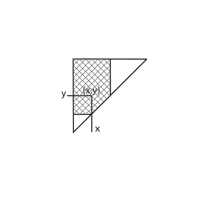
Figure 2. For a given $(x,y)$ in ${\mathcal{S}}$, the relevant $(x^{\prime},y^{\prime})$ that will give an edge in the intersection graph are in the hatched area.

The main theorem is stated in Section 3, and results on the chromatic number and clique number are given in Section 4. Some important preliminaries on continuity of the mapping $\mu\mapsto\Gamma_{\mu}$ are dealt with in Section 5, and Section 6 gives the proof of the main theorem. Section 7 discusses some examples of interval graph limits and the corresponding random interval graphs. The parametrization of graph limits is highly non unique; this is seen in some of the examples in Section 7. Section 8 gives a portemanteau theorem which clarifies the connections between various uniqueness results. This is developed for the general case, not just interval graphs. The problem of finding a unique “canonical” representing measure is still open in general. Section 9 gives the proofs of the results on clique numbers. Finally, Section 10 discusses extensions to other classes of intersection graphs, in particular circular-arc graphs, circle graphs, permutation graphs and unit interval graphs.

2. Background

This section gives background and references, treating interval graphs in Sections 2.1 and 2.2, random interval graphs in Section 2.3 and graph limits in Section 2.4–2.5.

2.1. Interval Graphs

Interval graphs and the closely associated subject of interval orders are a standard topic in combinatorics. A book length treatment of the subject is given by Fishburn [14]. Among many other results, we mention that interval graphs are perfect graphs, i.e., the chromatic number equals the size of the largest clique (for the graph and all induced subgraphs).

Interval graphs are a special case of intersection graphs; more generally, we may consider a collection $\mathcal{A}$ of subsets of some universe and the class of graphs that can be defined by replacing intervals by elements of $\mathcal{A}$ in the definition above. (We may call such graphs $\mathcal{A}$-intersection graphs.)

McKee and McMorris [32]’s book on Intersection Graphs establishes the relation with intervals. Further literature on the connections between these various graph classes is in Brandstädt, Le and Spinrad [9] and Golumbic [18].

2.2. Applications of Interval Graphs

The original question for which interval graphs saw their first application was in the structure of genetic DNA. Waterman and Griggs [42] and Klee [29] cite Benzer’s original paper from 1959 [2]. This is also developed in the papers by Karp [28] and Golumbic et al. [19]. Interval graphs are used for censored and truncated data; the interval indicating for instance observed lifetime (see Gentleman and Vandal [15] and the R packages MLEcens and lcens). They also come in when restricting data - like permutations - to certain observable intervals, this was the motivation behind the astrophysics paper Efron and Petrosian [13] and the followup paper Diaconis et al. [10]. For an application of rectangle intersections, see Rim and Nakajima [36] and for sphere intersections see Ghrist [16].

2.3. Random Interval Graphs

A natural model of random interval graphs has $[a_{i},b_{i}]$ chosen uniformly at random inside [0,1]. Scheinerman [38] shows that

$$\#\text{edges} =\frac{n^{2}}{3}+o_{p}(n^{2}),$$ (2.1)

$$\operatorname{\mathbb{P}{}}\Bigl{\{}\frac{\min_{v}\deg(v)}{\sqrt{n}}\leq x\Bigr{\}} \longrightarrow 1-e^{-x^{2}/2},\qquad x>0,$$ (2.2)

and, if $v$ is a fixed vertex,

$$\operatorname{\mathbb{P}{}}\Bigl{\{}\frac{\deg(v)}{n}\leq x\Bigr{\}}\rightarrow\begin{cases}1-(1-x)\frac{\pi}{2},&x\geq\frac{1}{2};\\ 1-(1-x)\left\{\frac{\pi}{2}-2\cos^{-1}[\frac{1}{\sqrt{2-2x}}]\right\}-\sqrt{1-2x},&x<\frac{1}{2}.\\ \end{cases}$$ (2.3)

He further shows that most such graphs are connected, indeed Hamiltonian, the chromatic number is $\frac{n}{2}+o_{p}(n)$ and several other things; see also Justicz, Scheinerman and Winkler [24] where it is shown that the maximum degree is $n-1$ with probability exactly $2/3$ for any $n>1$. The chromatic number equals, as said in Section 2.1, the size of the largest clique, and this is equivalent to the random sock sorting problem studied by Steinsaltz [41] and Janson [20] where more refined results are shown, including asymptotic normality which for the random interval graph $G_{n}$ considered here can be written $(\chi(G_{n})-n/2)/\sqrt{n}\to N(0,1/4)$.

We connect this random interval graph to graph limits in Example 7.4, where also other models of random interval graphs are considered.

There has been some followup on this work with Scheinerman [39] introducing an evolving family of models, and Godehardt and Jaworski [17] studying independence numbers of random interval graphs for cluster discovery. Pippenger [35] has studied other models with application to allocation in multi-sever queues. Here, customers arrive according to a Poisson process, the service time distribution determines an interval length distribution and the intervals, falling into a given window give an interval graph. For natural models, those graphs are sparse, in contrast to our present study of dense graphs.

Finally we give a pointer to an emerging literature on random intersection graphs where subsets of size $d$ from a finite set are chosen uniformly for each vertex and there is an edge between two vertices if the subsets have a non empty intersection. See results and references in [27] and [40].

2.4. Graph Limits

This paper studies limits of interval graphs, using the theory of graph limits introduced by Lovász and Szegedy [30] and further developed in Borgs, Chayes, Lovász, Sós and Vesztergombi [7, 8] and other papers by various combinations of these and other authors; see also Austin [1] and Diaconis and Janson [12]. We refer to these papers for the detailed definitions, which may be summarized as follows (using the notation of [12]).

If $F$ and $G$ are two graphs, then $t(F,G)$ denotes the probability that a random mapping $\phi:V(F)\to V(G)$ defines a graph homomorphism, i.e., that $\phi(v)\phi(w)\in E(G)$ when $vw\in E(F)$. (By a random mapping we mean a mapping uniformly chosen among all $|G|^{|F|}$ possible ones; the images of the vertices in $F$ are thus independent and uniformly distributed over $V(G)$, i.e., they are obtained by random sampling with replacement.) The basic definition is that a sequence $G_{n}$ of graphs converges if $t(F,G_{n})$ converges for every graph $F$; we will use the version in [12] where we further assume $|G_{n}|\to\infty$. More precisely, the (countable and discrete) set ${\mathcal{U}}$ of all unlabeled graphs can be embedded in a compact metric space $\overline{{\mathcal{U}}}$ such that a sequence $G_{n}\in{\mathcal{U}}$ of graphs with $|G_{n}|\to\infty$ converges in $\overline{{\mathcal{U}}}$ to some limit $\Gamma\in\overline{{\mathcal{U}}}$ if and only if $t(F,G_{n})$ converges for every graph $F$. Let ${\mathcal{U}}_{\infty}:=\overline{{\mathcal{U}}}\setminus{\mathcal{U}}$ be the set of proper graph limits. The functionals $t(F,\cdot)$ extend to continuous functions on $\overline{{\mathcal{U}}}$, and an element $\Gamma\in{\mathcal{U}}_{\infty}$ is determined by the numbers $t(F,\Gamma)$. Hence, $G_{n}\to\Gamma\in{\mathcal{U}}_{\infty}$ if and only if $|G_{n}|\to\infty$ and $t(F,G_{n})\to t(F,\Gamma)$ for every graph $F$. (See [7; 8] for other, equivalent, characterizations of $G_{n}\to\Gamma$.)

We say that a graph limit $\Gamma\in{\mathcal{U}}_{\infty}$ is an interval graph limit if $G_{n}\to\Gamma$ for some sequence of interval graphs. The purpose of the present paper is to study this class of graph limits.

Remark 2.1.

In Diaconis, Holmes and Janson [11], the corresponding problem for the class ${\mathcal{T}}$ of threshold graphs is studied. Recall that a graph is a threshold graph [33] if there are real valued vertex labels $v_{i}$ and a threshold $t$ such that $(i,j)$ is an edge if and only if $v_{i}+v_{j}\leq t$. Equivalently, the graph can be built up sequentially by adding vertices which are either dominating (connected to all previous vertices) or isolated (disjoint from all previous vertices). Threshold graphs are a subclass of interval graphs; this can be seen from the sequential description by choosing a sequence of intervals overlapping all previous or disjoint from all previous intervals as required. Thus every threshold graph limit is an interval graph limit. The description of threshold graph limits in [11] uses special properties of threshold graphs, and is of a somewhat different type than the descriptions of interval graph limits in the present paper. Thus, a threshold graph limit may be represented both as in [11] and as in the present paper, and the representations will not be the same. (This is nothing strange, since the representations typically are non-unique.)

Let $\mathcal{I}\subset{\mathcal{U}}$ be the set of all interval graphs, and let $\mathcal{I}_{\infty}\subset{\mathcal{U}}_{\infty}$ be the set of all interval graph limits; further, let $\overline{\mathcal{I}}\subset\overline{{\mathcal{U}}}$ be the closure of $\mathcal{I}$ in $\overline{{\mathcal{U}}}$. Then $\mathcal{I}_{\infty}=\overline{\mathcal{I}}\cap{\mathcal{U}}_{\infty}=\overline{\mathcal{I}}\setminus\mathcal{I}$. Clearly, $\mathcal{I}_{\infty}$ is a closed subset of ${\mathcal{U}}_{\infty}$ and thus a compact metric space.

A graph limit $\Gamma\in{\mathcal{U}}_{\infty}$ may be represented as follows [30], see also [12; 1] for connections to the Aldous–Hoover representation theory for exchangeable arrays [26]. Let $({\mathcal{S}},\mu)$ be an arbitrary probability space and let $W:{\mathcal{S}}\times{\mathcal{S}}\to[0,1]$ be a symmetric measurable function. ($W$ is sometimes called graphon [7; 8], we will use the alternative kernel denomination [4].) Let $X_{1},X_{2},\dots,$ be an i.i.d. sequence of random elements of ${\mathcal{S}}$ with common distribution $\mu$. Then there is a (unique) graph limit $\Gamma\in{\mathcal{U}}_{\infty}$ with, for every graph $F$,

$$\begin{split}t(F,\Gamma)&=\operatorname{\mathbb{E}{}}\prod_{ij\in E(F)}W(X_{i},X_{j})\\ &=\int_{{\mathcal{S}}^{|F|}}\prod_{ij\in E(F)}W(x_{i},x_{j})\,\textup{d}\mu(x_{1})\dotsm\,\textup{d}\mu(x_{|F|}).\end{split}$$ (2.4)

Further, let, for every $n\geq 1$, $G(n,W,\mu)$ be the random graph obtained by first taking random $X_{1},X_{2},\dots,X_{n}$, and then, conditionally given $X_{1},X_{2},\allowbreak\dots,\allowbreak X_{n}$, for each pair $(i,j)$ with $i<j$ letting the edge $ij$ appear with probability $W(X_{i},X_{j})$, (conditionally) independently for all pairs $(i,j)$ with $i<j$. Then the random graph $G_{n}=G(n,W,\mu)$ converges to $\Gamma$ a.s. as ${n\to\infty}$.

Conversely, every graph limit $\Gamma\in{\mathcal{U}}_{\infty}$ can be represented in this way by some such $({\mathcal{S}},\mu)$ and $W$. (The representation is not unique, see Section 8.)

Remark 2.2.

For any random graph $G(n,W,\mu)$ (not just interval graphs) the number of copies of any fixed subgraph (e.g.  triangles) is a U-statistic, perhaps with extra randomization if $W$ takes on values other than 0 or 1. Thus central limit theorems with error estimates and correction terms as well as large deviation results are available.

It is usually convenient to fix $({\mathcal{S}},\mu)$ and let $W:{\mathcal{S}}^{2}\to[0,1]$ vary; the standard choice of $({\mathcal{S}},\mu)$ is the unit interval $[0,1]$ with Lebesgue measure $\lambda$. (Every graph limit can be represented as in (2.4) using this space.) For interval graphs, however, we find it more natural and convenient to instead fix ${\mathcal{S}}$ and $W$ as follows, and let $\mu$ vary.

There is some flexibility in the definition above of interval graphs. The intervals in the definition may be arbitrary intervals of real numbers, or more generally intervals in any totally ordered set, but we may without changing the class of interval graphs restrict the intervals to be, for example, closed. We may also suppose that all intervals are subsets of $[0,1]$. It may sometimes be convenient to allow an empty interval $\emptyset$ (for isolated vertices), but we find it more convenient (at least notationally) to abstain from this and consider non-empty intervals only. We will, however, allow “intervals” $[a,a]=\{a\}$ of length 0.

Consequently, from now and throughout the paper (except where stated otherwise) we let ${\mathcal{S}}:=\{[a,b]:0\leq a\leq b\leq 1\}$ be the set of closed subintervals of $[0,1]$ (non-empty, but allowing intervals of length 0). ${\mathcal{S}}$ is naturally identified with a closed triangle in the plane, and is thus a compact metric space. (It is the compactness that makes this space better for our purposes than, for example, the space of all closed intervals in $\mathbb{R}$.) Further, we let from now on $W:{\mathcal{S}}\times{\mathcal{S}}\to\{0,1\}$ be the function

$$W(I,J)=\boldsymbol{1}[I\cap J\neq\emptyset].$$ (2.5)

Then, a graph $G=(V,E)$ is an interval graph if and only if there exist intervals $I_{v}\in{\mathcal{S}}$, $v\in V$, such that the edge indicators $\boldsymbol{1}[vw\in E]=W(I_{v},I_{w})$, $v\neq w$.

Every probability measure $\mu$ on ${\mathcal{S}}$ defines a graph limit $\Gamma\in{\mathcal{U}}_{\infty}$ by (2.4); we denote this graph limit by $\Gamma_{\mu}$. Similarly, we denote the random graph $G(n,W,\mu)$ constructed from $({\mathcal{S}},\mu)$ and $W$ by $G(n,\mu)$; this is simply the random interval graph defined by a random i.i.d. sequence of intervals $X_{1},X_{2},\dots,X_{n}$ with distribution $\mu$; we further allow $n=\infty$ here, and let $G(\infty,\mu)$ be the random infinite graph defined in the same way by $X_{1},X_{2},\dots$. (In [12], the standard situation when ${\mathcal{S}}$ and $\mu$ are fixed, we instead use the notations $\Gamma_{W}$ and $G(n,W)$; we will also use that notation when we discuss general functions $W$ again in Section 8.) Hence, by the general results quoted above, $G(n,\mu)\to\Gamma_{\mu}$ a.s. as ${n\to\infty}$. In particular, $\Gamma_{\mu}$ is an interval graph limit: $\Gamma_{\mu}\in\mathcal{I}_{\infty}$ for every probability measure $\mu$ on ${\mathcal{S}}$.

Remark 2.3.

A graph $G\in{\mathcal{U}}$ corresponds to a ’ghost’ $\Gamma_{G}\in{\mathcal{U}}_{\infty}$ with $t(F,\Gamma_{G})=t(F,G)$ for all $F$ [30; 12]. If $G$ is an interval graph represented by a sequence $I_{1},\dots,I_{n}$ of intervals in ${\mathcal{S}}$ (with $n=|G|$), then it follows easily from (2.4) that $\Gamma_{G}=\Gamma_{\mu}$, where $\mu=\frac{1}{n}\sum_{1}^{n}\delta_{I_{i}}$ is the distribution of a random interval chosen uniformly from $I_{1},\dots,I_{n}$.

Our main theorem (Theorem 3.1) gives a converse: every interval graph limit can be represented by a probability $\mu$ on ${\mathcal{S}}$; moreover, we may impose a normalization. (In fact, we have a choice between three different normalizations.) However, even with one of these normalizations, the representing measure is not always unique.

Remark 2.4.

For every measure $\mu$ on ${\mathcal{S}}$ we thus have a model $G(n,\mu)$ of random interval graphs. Different measures $\mu$ give the same model (i.e., with the same distribution for every $n$) if and only if they give the same graph limit $\Gamma_{\mu}$, see Section 8. We may thus construct a large number of different models of random interval graphs in this way. We give a few examples in Section 7.

2.5. Degree distribution

Suppose that $G_{n}$ is a sequence of graphs with, for convenience, $|G_{n}|=n$, such that $G_{n}\to\Gamma$ for a graph limit $\Gamma$ which is represented by a kernel $W$ on a probability space $({\mathcal{S}},\mu)$. (In this subsection $W$ and ${\mathcal{S}}$ may be arbitrary.) Let $\bar{d}(G_{n})=2e(G_{n})/n$ be the average degree of $G_{n}$. It follows immediately $\bar{d}(G_{n})/n$ converges to the average $\int_{{\mathcal{S}}^{2}}W(x_{1},x_{2})\,\textup{d}\mu(x_{1})\,\textup{d}\mu(x_{2})$; in fact, $\bar{d}(G_{n})/n=2e(G_{n})/n^{2}=t(K_{2},G_{n})\to t(K_{2},\Gamma)=\int_{{\mathcal{S}}^{2}}W$. (Equivalently, the edge density $e(G_{n})/\binom{n}{2}\to\int_{{\mathcal{S}}^{2}}W$.)

Moreover, let $\nu(G_{n})$ be the normalized degree distribution of $G_{n}$, defined as the distribution of the random variable $d_{i}/n$, where $i$ is a uniformly random vertex in $G_{n}$ and $d_{i}$ its degree. Then $\nu(G_{n})$ converges weakly (as a probability measure on $[0,1]$) to the distribution of the random variable $W_{1}(X):=\int_{\mathcal{S}}W(X,z)\,\textup{d}\mu(z)$, where $X$ is a random element of ${\mathcal{S}}$ with distribution $\mu$; note that $W_{1}(X)\in[0,1]$ and that its mean is $\int_{{\mathcal{S}}^{2}}W$. We can thus regard the distribution of this random variable $W_{1}(X)$ as the degree distribution of the graph limit; we denote it by $\nu(\Gamma)$ or (in our case, where $W$ is fixed) $\nu(\mu)$. See for example [11].

In particular, for any given $\mu$ on our standard ${\mathcal{S}}$, this applies a.s. to the random interval graphs $G(n,\mu)$, since $G(n,\mu)\to\Gamma_{\mu}$ as said above.

3. Interval Graph Limits, Theorems

Let $\mathcal{P}({\mathcal{S}})$ be the set of probability measures on ${\mathcal{S}}:=\{[a,b]:0\leq a\leq b\leq 1\}$, equipped with the standard topology of weak convergence, which makes $\mathcal{P}({\mathcal{S}})$ a compact metric space. If $\mu\in\mathcal{P}({\mathcal{S}})$, let $\mu_{L}$ and $\mu_{R}$ be the marginals of $\mu$ (regarding ${\mathcal{S}}$ as a subset of $\mathbb{R}^{2}$), i.e., the probability measures on $[0,1]$ induced by $\mu$ and the mappings ${\mathcal{S}}\to[0,1]$ given by $[a,b]\mapsto a$ and $[a,b]\mapsto b$, respectively.

We further consider, both as normalizations and for reasons of continuity, see Corollary 5.2 below, three subsets of $\mathcal{P}({\mathcal{S}})$: (as above, $\lambda$ denotes Lebesgue measure, i.e., the uniform distribution)

$$\mathcal{P}_{L}({\mathcal{S}}) :=\{\mu\in\mathcal{P}({\mathcal{S}}):\mu_{L}=\lambda\},$$ (3.1)

$$\mathcal{P}_{R}({\mathcal{S}}) :=\{\mu\in\mathcal{P}({\mathcal{S}}):\mu_{R}=\lambda\},$$ (3.2)

$$\mathcal{P}_{m}({\mathcal{S}}) :=\{\mu\in\mathcal{P}({\mathcal{S}}):\tfrac{1}{2}(\mu_{L}+\mu_{R})=\lambda\}.$$ (3.3)

We have the following result, which is proved in Section 6.

Theorem 3.1.

$\mathcal{I}_{\infty}=\{\Gamma_{\mu}:\mu\in\mathcal{P}({\mathcal{S}})\}$. Moreover, every $\Gamma\in\mathcal{I}_{\infty}$ may be represented as $\Gamma_{\mu}$ where we further may impose any one of the normalization conditions in (3.1)–(3.3). In other words,

$$\mathcal{I}_{\infty}=\{\Gamma_{\mu}:\mu\in\mathcal{P}_{L}({\mathcal{S}})\}=\{\Gamma_{\mu}:\mu\in\mathcal{P}_{R}({\mathcal{S}})\}=\{\Gamma_{\mu}:\mu\in\mathcal{P}_{m}({\mathcal{S}})\}.$$

Furthermore, the mapping $\mu\to\Gamma_{\mu}$ is a continuous map of each of $\mathcal{P}_{L}({\mathcal{S}})$, $\mathcal{P}_{R}({\mathcal{S}})$ and $\mathcal{P}_{m}({\mathcal{S}})$ onto $\mathcal{I}_{\infty}$.

The mappings $\mathcal{P}_{L}({\mathcal{S}})\to\mathcal{I}_{\infty}$, $\mathcal{P}_{R}({\mathcal{S}})\to\mathcal{I}_{\infty}$, $\mathcal{P}_{m}({\mathcal{S}})\to\mathcal{I}_{\infty}$ are not injective. We return to this question in Sections 7 and 8.

The proof in Section 6 also shows the following, which gives an interpretation of the measure $\mu$.

Theorem 3.2.

Let $G_{n}$ be an interval graph, for convenience with $n$ vertices, defined by intervals $I_{ni}=[a_{ni},b_{ni}]\subseteq[0,1]$, $i=1,\dots,n$. Suppose that, as ${n\to\infty}$, the empirical measure

$$\mu_{n}:=\frac{1}{n}\sum_{i=1}^{n}\delta_{I_{ni}}\in\mathcal{P}({\mathcal{S}})$$ (3.4)

converges weakly to a measure $\mu\in\mathcal{P}({\mathcal{S}})$, and suppose further that $\mu_{L}$ and $\mu_{R}$ have no common atom. Then $G_{n}$ converges to the graph limit $\Gamma_{\mu}$.

Instead of probability measures $\mu\in\mathcal{P}({\mathcal{S}})$, we may equivalently consider ${\mathcal{S}}$-valued random variables, i.e., random intervals $[L,R]\in{\mathcal{S}}$. Each such random interval is given by a pair of random variables $(L,R)$ with $0\leq L\leq R\leq 1$ (a.e.), and conversely. (Of course, we then only care about the (joint) distribution of $(L,R)$.) Note that the distribution of $[L,R]$ belongs to $\mathcal{P}_{L}({\mathcal{S}})$ [$\mathcal{P}_{R}({\mathcal{S}})$] if and only if $L\sim\textsf{U}(0,1)$ [$R\sim\textsf{U}(0,1)$].

Example 3.3.

A natural model for a collection of confidence intervals for a basic physical constant (as Youden’s data in the introduction or the speed of light or the gravitational constant) has intervals of the form $[\mu_{i}-c\sigma_{i},\mu_{i}+c\sigma_{i}]$ with $\mu_{i}$ and $\sigma_{i}$ independently chosen, $\mu_{i}$ from a normal $(\mu,\sigma^{2})$ distribution and $\sigma_{i}^{2}$ from a Chi-squared distribution, $c$ is computed from the normal quantile $q$ and the sample size $c=q_{1-\frac{\alpha}{2}}/\sqrt{n}$, where $\alpha$ is the target type I error. Here the intervals are not constrained to ${\mathcal{S}}$. A natural transformation using the distribution function $F(x)$ of $\mu_{i}+c\sigma_{i}$ yields the random intervals $[F^{-1}(\mu_{i}-c\sigma_{i}),F^{-1}(\mu_{i}+c\sigma_{i})]$, which correspond to points from a distribution on ${\mathcal{S}}$ belonging to our $\operatorname{\mathbb{P}{}}_{R}({\mathcal{S}})$.

An example, with $\mu_{i}\sim N(0,4)$ and $\sigma^{2}_{i}\sim\frac{4}{19}\chi^{2}_{19}$ is given in Figure 3.

(a) Confidence Intervals (30) for random normal data generated with $\mu=0,\sigma=2$.

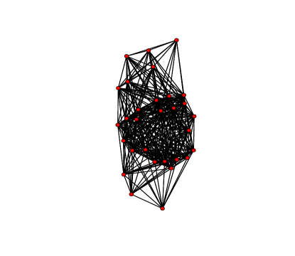
(b) Interval Graph

Figure 3. The interval graph for a sets of Normal intervals.

Although the graph is not the complete graph as it should be if all $30$ intervals overlapped, the degrees are high and quite even. The degree distribution is:

 22 20 25 26 23 14 23 23 27 23 26 25 26 27 13
 23 17 23 20 27 23 14 24 25 25 26 26 17 11 10

Remark 3.4.

There is an obvious reflection map of ${\mathcal{S}}$ onto itself given by $[a,b]\mapsto[1-b,1-a]$; we denote the corresponding map of $\mathcal{P}({\mathcal{S}})$ onto itself by $\mu\mapsto\check{\mu}$. (It terms of random intervals $[L,R]$, this is $[L,R]\mapsto[1-R,1-L]$.) The reflection map preserves $W$, and it follows that $\Gamma_{\check{\mu}}=\Gamma_{\mu}$.

Note that $\mu\in\mathcal{P}_{L}({\mathcal{S}})\iff\check{\mu}\in\mathcal{P}_{R}({\mathcal{S}})$, and conversely, which means that we can transfer results from $\mathcal{P}_{L}({\mathcal{S}})$ to $\mathcal{P}_{R}({\mathcal{S}})$, and conversely, by the reflection map; hence it is enough to consider one of $\mathcal{P}_{L}({\mathcal{S}})$ and $\mathcal{P}_{R}({\mathcal{S}})$.

Remark 3.5.

As a corollary to Theorem 3.1, we see that every limit of interval graphs may be represented by a kernel that is $0/1$-valued. (This implies that every representing kernel is $0/1$-valued, see [23] for details.) Graph classes with this property are called random-free by Lovász and Szegedy [31], who among other results gave a graph-theoretic characterization of such classes. We have thus shown that the class of interval graphs is random-free. We will see in Sections 10.1–10.4 that so are the graph classes considered there.

4. Cliques and chromatic number

If $G$ is a graph, let $\chi(G)$ be its chromatic number and $\omega(G)$ its clique number, i.e., the maximal size of a clique. As said in Section 2.1, interval graphs are perfect and $\chi(G)=\omega(G)$ for them. If $G$ is an interval graph defined by a collection of intervals $\{I_{i}\}$, it is easily seen that $\omega(G)=\max_{x}\#\{i:x\in I_{i}\}$. We define the corresponding quantity for measures $\mu\in\mathcal{P}({\mathcal{S}})$ by

$$\omega(\mu):=\sup_{a\in[0,1]}\mu\{I:a\in I\}=\sup_{a\in[0,1]}\mu\bigl{(}[0,a]\times[a,1]\bigr{)}.$$ (4.1)

Thus, if $G$ is an interval graph defined by intervals $I_{1},\dots,I_{n}$ in ${\mathcal{S}}$, and $\mu=\frac{1}{n}\sum_{i=1}^{n}\delta_{I_{i}}$, then $\omega(G)=n\omega(\mu)$.

It is easy to see that $a\mapsto\mu\bigl{(}[0,a]\times[a,1]\bigr{)}$ is upper semicontinuous; this implies that the supremum in (4.1) is attained.

We will prove the following results in Section 9.

Lemma 4.1.

If $\mu_{1}$ and $\mu_{2}$ are probability measures on ${\mathcal{S}}$ that are equivalent in the sense that $\Gamma_{\mu_{1}}=\Gamma_{\mu_{2}}$, then $\omega(\mu_{1})=\omega(\mu_{2})$.

This shows that we can define the clique number $\omega(\Gamma)$ for every interval graph limit $\Gamma$ by $\omega(\Gamma_{\mu})=\omega(\mu)$ for $\mu\in\mathcal{P}({\mathcal{S}})$.

Theorem 4.2.

Let $G_{n}$ be an interval graph, for convenience with $n$ vertices, and suppose that $G_{n}\to\Gamma$ as ${n\to\infty}$ for some graph limit $\Gamma$. Then

$$\frac{1}{n}\chi(G_{n})=\frac{1}{n}\omega(G_{n})\to\omega(\Gamma).$$ (4.2)

Remark 4.3.

Neither $\frac{1}{n}\chi$ nor $\frac{1}{n}\omega$ are continuous functions on the space of all graphs. This may be seen by the following construction: a sequence of dense graphs which tend to the limiting Erdös-Renyi graph with $p=1$ (complete graph) but with $\frac{1}{n}\chi$ and $\frac{1}{n}\omega$ converging to limits different from one. For the construction, let $G_{n}$ be an Erdös-Renyi graph with $p=1-\frac{1}{\sqrt{n}}$. This converges to the same limit as the sequence of complete graphs $K_{n}$. However, an easy argument shows that $\frac{1}{n}\omega$ converges to zero. The same example can be used to show that $\frac{1}{n}\chi$ is not continuous. For this we use the following

Lemma 4.4.

For any graph $G$ with $n$ vertices, $\chi(G)\leq(n+\omega(G))/2$

Proof.

Color by picking two non adjacent vertices, giving both the same new color. Repeat until a connected subgraph of size $m$ remains and give each remaining vertex a separate color. This uses $(n-m)/2+m=(n+m)/2$ colors and $m\leq\omega(G)$. ∎

For the random graphs constructed above, $\omega(G)=o(n)$ implies $\chi(G)\leq\frac{n}{2}+o(n)$. Thus $\frac{1}{n}\chi$ is discontinuous.

5. Continuity

The mapping $\mu\mapsto\Gamma_{\mu}$ of $\mathcal{P}({\mathcal{S}})$ into ${\mathcal{U}}_{\infty}$ is not continuous. However, the following holds, as we will prove below.

Theorem 5.1.

The mapping $\mu\mapsto\Gamma_{\mu}$ of $\mathcal{P}({\mathcal{S}})$ into ${\mathcal{U}}_{\infty}$ is continuous at every $\mu\in\mathcal{P}({\mathcal{S}})$ such that $\mu_{L}$ and $\mu_{R}$ have no common atom. Conversely, it is continuous only at these $\mu$.

In particular, $\Gamma_{\mu}$ is a continuous function of $\mu$ at every $\mu$ such that either $\mu_{L}$ or $\mu_{R}$ is continuous, which yields the following corollary.

Corollary 5.2.

The mapping $\mu\mapsto\Gamma_{\mu}$ is a continuous map $\mathcal{P}_{L}({\mathcal{S}})\to{\mathcal{U}}_{\infty}$, $\mathcal{P}_{R}({\mathcal{S}})\to{\mathcal{U}}_{\infty}$ and $\mathcal{P}_{m}({\mathcal{S}})\to{\mathcal{U}}_{\infty}$.

To prove Theorem 5.1, we begin by letting $D_{W}\subset{\mathcal{S}}^{2}$ be the set of discontinuity points of $W$.

Lemma 5.3.

$D_{W}=\bigl{\{}([a,b],[c,d]):b=c\text{ \rm or }a=d\bigr{\}}$.

Proof.

Obvious. ∎

Proof of Theorem 5.1.

Suppose that $\mu_{n}\to\mu$ in $\mathcal{P}({\mathcal{S}})$ and that $\mu_{L}$ and $\mu_{R}$ have no common atom. Then Lemma 5.3 implies that $\mu\times\mu(D_{W})=0$, and it follows that if $F\in{\mathcal{U}}$ and $k=|F|$, then $\prod_{ij\in E(F)}W(x_{i},x_{j}):{\mathcal{S}}^{k}\to\{0,1\}\subset\mathbb{R}$ is $\mu^{k}$-a.e. continuous. Further, $\mu_{n}^{k}\to\mu^{k}$ in $\mathcal{P}({\mathcal{S}}^{k})$, and thus $t(F,\Gamma_{\mu_{n}})\to t(F,\Gamma_{\mu})$ by (2.4), see [3, Theorem 5.2]. Hence, $\Gamma_{\mu_{n}}\to\Gamma_{\mu}$ by the definition of ${\mathcal{U}}_{\infty}$.

For the converse (which we will not use), assume that $a$ is a common atom of $\mu_{L}$ and $\mu_{R}$. By symmetry we may suppose that $a>0$. Let, for $n>1/a$, $a_{n}:=a-1/n$. If $\mu$ has an atom at $[a,a]$, we define $\mu_{n}$ by moving half of that atom to $[a_{n},a_{n}]$. Otherwise, we replace every interval $[c,a]$ with $c\leq a_{n}$ by $[c,a_{n}]$; this yields a map ${\mathcal{S}}\to{\mathcal{S}}$ which maps $\mu$ to a measure $\mu_{n}$. It is easy to see, in both cases, that $\mu_{n}\to\mu$ but, using (2.4),

$$t(K_{2},\Gamma_{\mu_{n}})=\int_{{\mathcal{S}}^{2}}W\,\textup{d}\mu_{n}\times\,\textup{d}\mu_{n}\not\to\int_{{\mathcal{S}}^{2}}W\,\textup{d}\mu\times\,\textup{d}\mu=t(K_{2},\Gamma_{\mu}).$$

Hence $\Gamma_{\mu_{n}}\not\to\Gamma_{\mu}$. ∎

6. Proof of Theorems 3.1 and 3.2

Proof of Theorem 3.2.

It follows from (2.4), see Remark 2.3, that

$$t(F,G_{n})=t(F,\Gamma_{\mu_{n}}),\qquad F\in{\mathcal{U}}.$$ (6.1)

Theorem 5.1 shows that $\Gamma_{\mu_{n}}\to\Gamma_{\mu}$, i.e., $t(F,\Gamma_{\mu_{n}})\to t(F,\Gamma_{\mu})$ for every $F\in{\mathcal{U}}$. By (6.1), this implies $t(F,G_{n})\to t(F,\Gamma_{\mu})$, $F\in{\mathcal{U}}$, and thus $G_{n}\to\Gamma_{\mu}$. ∎

Proof of Theorem 3.1.

If $\mu\in\mathcal{P}({\mathcal{S}})$, then as said in Section 2.4, $\Gamma_{\mu}$ is the limit a.s. of the sequence $G(n,\mu)$ of interval graphs, and thus $\Gamma_{\mu}\in\mathcal{I}_{\infty}$.

Conversely, if $G_{n}$ is a sequence of interval graphs and $G_{n}\to\Gamma\in{\mathcal{U}}_{\infty}$, then each $G_{n}$ is represented by some sequence of closed intervals $I_{ni}=[a_{ni},b_{ni}]\subset\mathbb{R}$, $i=1,\dots,n$. By, if necessary, increasing the lengths of these interval by small (and, e.g., random) amounts, we may further assume that for each $n$, the $2n$ endpoints $\{a_{ni},b_{ni}:1\leq i\leq n\}$ are distinct.

Using an increasing homeomorphism $\varphi_{n}$ of $\mathbb{R}$ onto itself, we may further assume that the left endpoints $\{a_{ni}:1\leq i\leq n\}$ are the points $\{j/n:0\leq j<n\}$ in some order, and further that all endpoints $b_{ni}\leq 1$. Thus $I_{ni}\in{\mathcal{S}}$ for every $i$. Let $\mu_{n}\in\mathcal{P}({\mathcal{S}})$ be the corresponding probability measure given by (3.4).

Since ${\mathcal{S}}$ is compact, the sequence $\mu_{n}$ is automatically tight, and there exists a probability measure $\mu\in\mathcal{P}({\mathcal{S}})$ such that, at least along a subsequence, $\mu_{n}\to\mu$. As a consequence, $\mu_{nL}\to\mu_{L}$, and since we have forced $\mu_{nL}$ to be the uniform measure on the set $\{j/n:j=0,\dots,n-1\}$, the limit $\mu_{L}=\lambda$. Hence $\mu\in\mathcal{P}_{L}({\mathcal{S}})$.

Consequently, Theorem 3.2 applies and shows that (along the subsequence) $G_{n}\to\Gamma_{\mu}$. Hence $\Gamma=\Gamma_{\mu}$.

This shows that every $\Gamma\in\mathcal{I}_{\infty}$ equals $\Gamma_{\mu}$ for some $\mu\in\mathcal{P}_{L}({\mathcal{S}})$. The same argument but choosing the homeomorphism $\varphi_{n}$ of $\mathbb{R}$ onto itself such that the right endpoints or all $2n$ endpoints are evenly spaced in $[0,1]$ similarly yields $\Gamma=\Gamma_{\mu}$ with $\mu\in\mathcal{P}_{R}({\mathcal{S}})$ or $\mu\in\mathcal{P}_{m}({\mathcal{S}})$.

This, combined with Corollary 5.2, completes the proof of Theorem 3.1. ∎

7. Examples

As is well-known, representations as in Section 1 of graph limits by symmetric measurable functions $W$ on a probability space are far from unique, see e.g., [30; 7; 12] and Section 8.

In particular, an interval graph limit $\Gamma\in\mathcal{I}$ may be represented as $\Gamma_{\mu}$ for many different $\mu\in\mathcal{P}({\mathcal{S}})$. For example, any monotone (increasing or decreasing) homeomorphism $[0,1]\to[0,1]$ induces a homeomorphism of ${\mathcal{S}}$ onto itself which preserves $W$, and hence maps any $\mu\in\mathcal{P}({\mathcal{S}})$ to a measure $\mu^{\prime}$ with $\Gamma_{\mu}=\Gamma_{\mu^{\prime}}$. (One example of such a homeomorphism of ${\mathcal{S}}$ onto itself is the reflection map in Remark 3.4, induced by the map $x\to 1-x$.)

If we use one of the normalizations in (3.1)–(3.3) and consider only $\mathcal{P}_{L}({\mathcal{S}})$, $\mathcal{P}_{R}({\mathcal{S}})$ or $\mathcal{P}_{m}({\mathcal{S}})$, the possibilities are severly restricted, and we have uniqueness in some cases, but not all.

Example 7.1.

The complete graph $K_{n}$ is an interval graph, and can be represented by any family of intervals that contain a common point. The sequence converges to a graph limit $\Gamma\in\mathcal{I}$. On the standard space $[0,1]$, $\Gamma$ is simply represented by the function $[0,1]^{2}\to[0,1]$ that is identically 1, but we are are interested in representations as $\Gamma_{\mu}$ for $\mu\in\mathcal{P}({\mathcal{S}})$. Clearly, $\Gamma=\Gamma_{\mu}$ for any $\mu\in\mathcal{P}({\mathcal{S}})$ such that there exists a point $c\in[0,1]$ with $\mu$ supported on the set $\{[a,b]:a\leq c\leq b\}$.

It is easily seen that there is a unique representation with $\mu\in\mathcal{P}_{L}({\mathcal{S}})$; $\mu$ is the distribution of $[U,1]$ with $U\sim\textsf{U}(0,1))$.

Similarly (and equivalently by reflection), there is a unique representation with $\mu\in\mathcal{P}_{R}({\mathcal{S}})$; $\mu$ is the distribution of $[0,U]$ with $U\sim\textsf{U}(0,1)$.

However, there are many representations with $\mu\in\mathcal{P}_{m}({\mathcal{S}})$; these are given by random intervals $[L,R]$ where $(L,R)$ has any joint distribution with the marginals $L\sim\textsf{U}(0,\frac{1}{2})$ and $R\sim\textsf{U}(\frac{1}{2},1)$.

Example 7.2.

Consider the disjoint union of two complete graphs with $\lfloor an\rfloor$ and $n-\lfloor an\rfloor$ vertices, where $0<a<1/2$. This sequence of graphs converges as ${n\to\infty}$ to a graph limit that is represented by two measures in $\mathcal{P}_{L}({\mathcal{S}})$, with corresponding random intervals $[L,R]$ where $L\sim\textsf{U}(0,1)$ and $R$ is given by either

$$R:=\begin{cases}a,&L\leq a,\\ 1,&L>a,\end{cases}$$

or the same formula with $a$ replaced by $1-a$. It can be seen that these two measures are the only measures in $\mathcal{P}_{L}({\mathcal{S}})$ representing the graph limit. (This is an example of a sum of two graph limits; see [21] for general results on such sums and decompositions.)

Example 7.3.

More generally, let $(p_{i})_{1}^{m}$ be a finite or infinite sequence of positive numbers with sum 1. Let $G_{n}$ be the interval graph consisting of disjoint complete graphs of orders $\lfloor np_{1}\rfloor$, $\lfloor np_{2}\rfloor$, …. (Hence, $|G_{n}|=n-o(n)$.) It is easily seen that $G_{n}\to\Gamma$ for some $\Gamma\in{\mathcal{U}}_{\infty}$; thus $\Gamma\in\mathcal{I}$. (Again, cf. [21].)

To represent $\Gamma$ as $\Gamma_{\mu}$ with $\mu\in\mathcal{P}_{L}({\mathcal{S}})$, let $(J_{i})_{1}^{m}$ be a partition of $(0,1]$ into disjoint intervals $J_{i}=(a_{i},b_{i}]$ with $\lambda(J_{i})=p_{i}$. Then, if $L\sim\textsf{U}(0,1)$ and $R$ is defined by $R:=b_{i}$ when $L\in J_{i}$, the random interval $[L,R]$ represents $\Gamma$. If $m<\infty$ and $p_{1},\dots,p_{m}$ are distinct, this gives $m!$ different measures $\mu\in\mathcal{P}_{L}({\mathcal{S}})$ representing the same $\Gamma_{\mu}$, since the intervals $J_{i}$ may come in any order. If $m=\infty$, we have an infinite number of different representations.

Example 7.4.

The random interval graph studied by Scheinerman [38], see Section 2.3, is defined as $G(n,\mu)$ where $\mu\in\mathcal{P}({\mathcal{S}})$ is the uniform measure on ${\mathcal{S}}$; thus $\mu$ has the density $2\,\textup{d}x\,\textup{d}y$ on $0\leq x\leq y\leq 1$. Note that the marginal distributions $\mu_{L}$ and $\mu_{R}$ have densities $2(1-x)$ and $2x$ on [0,1], and are thus not uniform. Hence $\mu\notin\mathcal{P}_{L}({\mathcal{S}})$ and $\mu\notin\mathcal{P}_{R}({\mathcal{S}})$; however, $\mu\in\mathcal{P}_{m}({\mathcal{S}})$.

The integral $W_{1}([x,y]):=\int_{\mathcal{S}}W([x,y],J)\,\textup{d}\mu(J)=1-x^{2}-(1-y)^{2}$; this leads by Section 2.5 and a calculation to the degree distribution (2.3) found by Scheinerman [38].

It is easily seen that $\omega(\mu)=1/2$, and thus Theorem 4.2 yields Scheinerman’s result that $\chi(G(n,\mu))/n\to 1/2$ (with convergence a.s.).

To obtain an equivalent representing measure $\mu^{\prime}\in\mathcal{P}_{R}({\mathcal{S}})$, we apply the homeomorphism $x\mapsto x^{2}$ of $[0,1]$ onto itself; this measure $\mu^{\prime}$ has the density $(2\sqrt{xy})^{-1}\,\textup{d}x\,\textup{d}y$ on ${\mathcal{S}}=\{[x,y]:0\leq x\leq y\leq 1\}$.

Example 7.5.

Scheinerman [39] studies another random interval graph model, defined by random intervals $[x_{i}-\rho_{i},x_{i}+\rho_{i}]$ where $x_{i}\sim\textsf{U}(0,1)$ and $\rho_{i}\sim\textsf{U}(0,r)$ are independent, and $r>0$ is a parameter. This is $G(n,\mu)$ where $\mu$ is the uniform distribution on the tilted rectangle with vertices in $(0,0)$, $(1,1)$, $(1-r,1+r)$, $(-r,r)$; this rectangle does not lie inside our standard triangle (i.e., the intervals are not necessarily inside $[0,1]$), but we may scale it to, for example, the rectangle with vertices $(0,\frac{2r}{1+2r})$, $(\frac{r}{1+2r},\frac{r}{1+2r})$, $(\frac{r+1}{1+2r},\frac{r+1}{1+2r})$, $(\frac{1}{1+2r},1)$. See Figure 4 for an example.

(a) Support

(b) Intervals

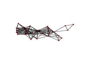
(c) Interval Graph

Figure 4. (A) shows support of $\mu$: tilted rectangle within ${\mathcal{S}}$. (B) shows the intervals with choice of parameters: 30 intervals, $r=0.2$. (C) shows the corresponding interval graph.

Example 7.6.

Let $0<r\leq 1$ and let $\mu$ be uniform on the line $\{(x,x+r):0\leq x\leq 1-r\}$. This is the set of intervals of length $r$ inside [0,1], so by scaling we obtain a random set of intervals of length 1 in $\mathbb{R}$; hence the random graph $G(n,\mu)$ is in this case a unit interval graph, see Section 10.4.

The degree distribution $\nu(\mu)$, i.e., the asymptotic degree destribution of the random graph $G(n,\mu)$, is easily found from Section 2.5. For example, if $r\leq\frac{1}{3}$, then $\nu(\mu)$ is the distribution of $W(X)$ with $X\sim\textsf{U}(0,1-r)$ and

$$W_{1}(x)=\begin{cases}\frac{x+r}{1-r},&0\leq x<r,\\ \frac{2r}{1-r},&r\leq x\leq 1-2r,\\ \frac{1-x}{1-r},&1-2r<x\leq 1-r.\end{cases}$$

Thus, $\nu(\mu)$ has a density $2$ on $[\frac{r}{1-r},\frac{2r}{1-r})$ and a point mass $\frac{1-3r}{1-r}$ at $\frac{2r}{1-r}$. If $\frac{1}{3}\leq r\leq\frac{1}{2}$, then similarly $\nu(\mu)$ has a density $2$ on $[\frac{r}{1-r},{1})$ and a point mass $\frac{3r-1}{1-r}$ at $1$. If $r\geq\frac{1}{2}$, then $G(n,\mu)$ is the complete graph and $\nu(\mu)$ is a point mass at 1.

The chromatic number is by Theorem 4.2 a.s. $\frac{r}{1-r}n+o(n)$ for $r\leq\frac{1}{2}$ (and trivially $n$ for $r\geq\frac{1}{2}$).

Example 7.7.

Theorem 3.1 shows that we can build any interval graph limit from a probability distribution $\mu$ on ${\mathcal{S}}:=\{[x,y]:0\leq x\leq y\leq 1\}$, with the marginal distribution of $\mu$ on the $y$ axis being uniform, i.e., $\mu\in\mathcal{P}_{R}({\mathcal{S}})$. Here is a hierarchy of examples of building such measures

1. As in Example 7.1 for the complete graph $K_{n}$. We take $\mu$ to be the uniform distribution on the $y$ axis. Repeated picks from $\mu$ correspond to intervals $[0,u_{i}]$ which all intersect.

2. The empty graph $E_{n}$ is an interval graph corresponding to disjoint intervals. Let $\mu$ be the uniform distribution on the $x=y$ diagonal. Repeated picks from $\mu$ yield intervals $[u_{i},u_{i}]$ which are disjoint with probability 1.

3. We may interpolate between these two examples, choosing $a$ with $0\leq a\leq 1$ and $\mu_{a}$ uniform on the line $\ell_{a}=\{(x,y):x=ay,\,0\leq y\leq 1\}$. This is done by picking intervals $[aU,U]$ with $U\sim\textsf{U}(0,1)$ so the $y$-margin $U$ is uniform on $[0,1]$. Now, some pairs of points on the line $\ell_{a}$ will result in edges and some not:
   For $[x_{1},y_{1}]$, $[x_{2},y_{2}]$ in ${\mathcal{S}}$, the intervals overlap iff $x_{1}\leq x_{2}\leq y_{1}$ or $x_{2}\leq x_{1}\leq y_{2}$. Equivalently if $x_{1}\leq x_{2}$ then $x_{2}\leq y_{1}$, or if $x_{1}\geq x_{2}$ then $y_{2}\leq x_{1}$. Here, the points on $\ell_{a}$ are $[ay_{1},y_{1}]$ and $[ay_{2},y_{2}]$, so there is overlap iff $ay_{1}\leq ay_{2}\leq y_{1}$ or $ay_{2}\leq ay_{1}\leq y_{2}$, or equivalently,

   $$ay_{1}\leq y_{2}\leq y_{1}/a.$$

   Thus the chance of an edge in this model is $\operatorname{\mathbb{P}{}}(aU_{1}\leq U_{2}\leq U_{1}/a)=2\operatorname{\mathbb{P}{}}(aU_{1}\leq U_{2}\leq U_{1})=1-a$.

   Moreover, by Section 2.5, the asymptotic degree distribution $\nu(\mu_{a})$ is the distribution of $W_{1}(U)$, where $U\sim\textsf{U}(0,1)$ and

   $$W_{1}(u)=\begin{cases}\bigl{(}\frac{1}{a}-a\bigr{)}u,&u\geq a,\\ 1-au,&a\leq u\leq 1.\end{cases}$$

   This distribution has density $a/(1-a^{2})$ on $[0,1-a]$ and $1/(a(1-a^{2}))$ on $[1-a,1-a^{2}]$ (for $a<1$). The chromatic number is by Theorem 4.2 a.s. asymptotic to $n\omega(\mu_{a})=(1-a)n$.

4. The next example of $\mu\in\mathcal{P}_{R}({\mathcal{S}})$ is a mixture of uniforms on $\ell_{a}$, where $a$ has a distribution on $[0,1]$. The prescription:

   • Pick $a=A$ at random from some distribution on $[0,1]$ and

   • independently pick uniformly on $\ell_{a}$,

   means that we pick intervals $[A,UA]$ with $A$ and $U$ independent and $U\sim\textsf{U}(0,1)$, while $A$ has any given distribution.

5. As an extreme example, consider the measure $\mu$ which is a $(\theta,1-\theta)$ mixture of uniform on $\ell_{0},\ell_{1}$, with $\theta\in[0,1]$. Then, identifying the vertices of $G(n,\mu)$ with the picked points in ${\mathcal{S}}$:

   • None of the points on $\ell_{1}$ have an edge between them.

   • All of the points on the line $\ell_{0}$ have edges between them.

   • Pairs of points, one from $\ell_{0}$, one from $\ell_{1}$ have an edge with probability $1/2$, but not independently. More precisely, there is an edge between $(0,u_{1})$ and $(u_{2},u_{2})$ iff $u_{1}\geq u_{2}$.

   It is easily seen that in this case, the random interval graph $G(n,\mu)$ is a threshold graph, see Remark 2.1; we may give $(0,u)$ label $u$ and $(u,u)$ label $-u$ and take the threshold $t=0$. (By [11, Corollary 6.7], $G(n,\mu)$ equals the random graph $T_{n,\theta}$ defined in [11].) Hence $\Gamma_{\mu}$ is a threshold graph limit in this case. (It is an open problem to characterize all $\mu\in\mathcal{P}({\mathcal{S}})$ such that $\Gamma_{\mu}$ is a threshold graph limit.)

6. Uniform intervals: As said in Example 7.4, the uniform distribution on ${\mathcal{S}}$ does not belong to $\mathcal{P}_{R}({\mathcal{S}})$, but it is equivalent to the distribution with density $(2\sqrt{xy})^{-1}\,\textup{d}x\,\textup{d}y$ which does. A change of variables to $(a,y)\in[0,1]^{2}$ with $a=x/y$ yields the density $\frac{1}{2}a^{-1/2}\,\textup{d}a\,\textup{d}y$, so this is of the type studied here, with $a$ having the $B(\frac{1}{2},1)$ distribution with density $\frac{1}{2}a^{-1/2}\,\textup{d}a$.

8. Uniqueness

We state a general equivalence theorem for representation of graph limits (not necessarily interval graph limits) by symmetric measurable functions. We therefore allow rather general probability spaces $({\mathcal{S}}_{1},\mu_{1})=({\mathcal{S}}_{2},\mu_{2})$ and general symmetric functions $W_{i}:{\mathcal{S}}_{i}^{2}\to[0,1]$ on them. In the standard case $({\mathcal{S}}_{1},\mu_{1})=({\mathcal{S}}_{2},\mu_{2})=([0,1],\lambda)$, parts (i)–(vii) of the theorem are given in [12] as a consequence of Hoover’s equivalence theorem for representations of exchangeable arrays Kallenberg [26, Theorem 7.28]. Other similar results are given by Bollobás and Riordan [5] and Borgs, Chayes and Lovász [6]; in particular, (viii) and (ix) below are modelled after similar results in Borgs, Chayes and Lovász [6]. A similar theorem is stated in Janson [23], and an almost identical theorem in the related case of partial orders is given in Janson [22].

We first introduce more notation. If $W_{2}:{\mathcal{S}}_{2}^{2}\to[0,1]$ and $\varphi:{\mathcal{S}}_{1}\to{\mathcal{S}}_{2}$, then $W_{2}^{\varphi}(x,y):=W_{2}(\varphi(x),\varphi(y))$.

A Borel space is a measurable space $({\mathcal{S}},\mathcal{F})$ that is isomorphic to a Borel subset of $[0,1]$, see e.g. [25, Appendix A1] and Parthasarathy [34]. In fact, a Borel space is either isomorphic to $([0,1],\mathcal{B})$ or it is countable infinite or finite. Moreover, every Borel subset of a Polish topological space (with the Borel $\sigma$-field) is a Borel space. A Borel probability space is a probability space $({\mathcal{S}},\mathcal{F},\mu)$ such that $({\mathcal{S}},\mathcal{F})$ is a Borel space.

If $W^{\prime}$ is a symmetric function ${{\mathcal{S}}^{2}}\to[0,1]$, where ${\mathcal{S}}$ is a probability space, we say following [6] that $x_{1},x_{2}\in{\mathcal{S}}$ are twins (for $W^{\prime}$) if $W^{\prime}(x_{1},y)=W^{\prime}(x_{2},y)$ for a.e. $y\in{\mathcal{S}}$. We say that $W^{\prime}$ is almost twin-free if there exists a null set $N\subset{\mathcal{S}}$ such that there are no twins $x_{1},x_{2}\in{\mathcal{S}}\setminus N$ with $x_{1}\neq x_{2}$.

In the theorem and its proof, we assume that $[0,1]$ is equipped with the measure $\lambda$, and ${\mathcal{S}}_{j}$ with $\mu_{j}$; for simplicity we do not always repeat this.

Theorem 8.1.

Suppose that $({\mathcal{S}}_{1},\mu_{1})$ and $({\mathcal{S}}_{2},\mu_{2})$ are two Borel probability spaces and that $W_{1}:{\mathcal{S}}_{1}^{2}\to[0,1]$ and $W_{2}:{\mathcal{S}}_{2}^{2}\to[0,1]$ are two symmetric measurable functions, and let $\Gamma_{1},\Gamma_{2}\in{\mathcal{U}}_{\infty}$ be the corresponding graph limits. Then the following are equivalent.

1. $\Gamma_{1}=\Gamma_{2}$ in ${\mathcal{U}}_{\infty}$.

2. $t(F,\Gamma_{1})=t(F,\Gamma_{2})$ for every graph $F$.

3. The exchangeable random infinite graphs $G(\infty,W_{1})$ and $G(\infty,W_{2})$ have the same distribution.

4. The random graphs $G(n,W_{1})$ and $G(n,W_{2})$ have the same distribution for every finite $n$.

5. There exist measure preserving maps $\varphi_{j}:[0,1]\to{\mathcal{S}}_{j}$, $j=1,2$, such that $W_{1}^{\varphi_{1}}=W_{2}^{\varphi_{2}}$ a.e., i.e., $W_{1}\bigl{(}\varphi_{1}(x),\varphi_{1}(y)\bigr{)}=W_{2}\bigl{(}\varphi_{2}(x),\varphi_{2}(y)\bigr{)}$ a.e. on $[0,1]^{2}$.

6. There exists a measurable mapping $\psi:{\mathcal{S}}_{1}\times[0,1]\to{\mathcal{S}}_{2}$ that maps $\mu_{1}\times\lambda$ to $\mu_{2}$ such that $W_{1}(x,y)=W_{2}\bigl{(}\psi(x,t_{1}),\psi(y,t_{2})\bigr{)}$ for a.e. $x,y\in{\mathcal{S}}_{1}$ and $t_{1},t_{2}\in[0,1]$.

7. $\delta_{\square}(W_{1},W_{2})=0$, where $\delta_{\square}$ is the cut metric defined in [7] (see also [5]).

If further $W_{2}$ is almost twin-free, then these are also equivalent to:

1. There exists a measure preserving map $\varphi:{\mathcal{S}}_{1}\to{\mathcal{S}}_{2}$ such that $W_{1}=W_{2}^{\varphi}$ a.s., i.e. $W_{1}{(x,y)}=W_{2}\bigl{(}\varphi(x),\varphi(y)\bigr{)}$ a.e. on ${\mathcal{S}}_{1}^{2}$.

If both $W_{1}$ and $W_{2}$ are almost twin-free, then these are also equivalent to:

1. There exists a measure preserving map $\varphi:{\mathcal{S}}_{1}\to{\mathcal{S}}_{2}$ such that $\varphi$ is a bimeasurable bijection of ${\mathcal{S}}_{1}\setminus N_{1}$ onto ${\mathcal{S}}_{2}\setminus N_{2}$ for some null sets $N_{1}\subset{\mathcal{S}}_{1}$ and $N_{2}\subset{\mathcal{S}}_{2}$, and $W_{1}=W_{2}^{\varphi}$ a.s., i.e. $W_{1}{(x,y)}=W_{2}\bigl{(}\varphi(x),\varphi(y)\bigr{)}$ a.e. on ${\mathcal{S}}_{1}^{2}$. If further $({\mathcal{S}}_{2},\mu_{2})$ has no atoms, for example if ${\mathcal{S}}_{2}=[0,1]$, then we may take $N_{1}=N_{2}=\emptyset$.

Note that (i)$\implies$(iv) implies that we can uniquely define the random graphs $G(n,\Gamma)$ for any graph limit $\Gamma$.

Proof.

(i)$\iff$(ii) holds by our definition of graph limits.

Next, the equivalences (i)$\iff$(ii)$\iff$(iii)$\iff$(iv)$\iff$(v)$\iff$(vi)$\iff$(vii) where shown in [12] in the special (but standard) case $({\mathcal{S}}_{1},\mu_{1})=({\mathcal{S}}_{2},\mu_{2})=([0,1],\lambda)$. Since every Borel space is either finite, countably infinite or (Borel) isomorphic to $[0,1]$, it is easily seen that there exist measure preserving maps $\gamma_{j}:[0,1]\to{\mathcal{S}}_{j}$, $j=1,2$. Then $W_{j}^{\gamma_{j}}:[0,1]^{2}\to[0,1]$, and it is easily seen that $\Gamma_{j}:=\Gamma_{W_{j}}=\Gamma_{W_{j}^{\gamma_{j}}}$ and $G(n,W_{j})\overset{\mathrm{d}}{=}G(n,W_{j}^{\gamma_{j}})$ for $n\leq\infty$, and further $\delta_{\square}(W_{j},W_{j}^{\gamma_{j}})=0$; hence (i)$\iff$(ii)$\iff$(iii)$\iff$(iv)$\iff$(vii) by the corresponding results for $[0,1]$.

If (i)–(iv) hold, then by (v) for $[0,1]$, there exist measure preserving functions $\varphi^{\prime}_{j}:[0,1]\to[0,1]$ such that $W_{1}^{\gamma_{1}}\bigl{(}\varphi^{\prime}_{1}(x),\varphi^{\prime}_{1}(y)\bigr{)}=W_{2}^{\gamma_{2}}\bigl{(}\varphi^{\prime}_{2}(x),\varphi^{\prime}_{2}(y)\bigr{)}$ a.e., and thus (v) holds with $\varphi_{j}:=\gamma_{j}\circ\varphi^{\prime}_{j}$.

Conversely, if (v) holds, then $G(n,W_{1})\overset{\mathrm{d}}{=}G(n,W_{1}^{\varphi_{1}})=G(n,W_{2}^{\varphi_{2}})\overset{\mathrm{d}}{=}G(n,W_{2})$ for every $n\leq\infty$; thus (v)$\implies$(iii),(iv).

(vi)$\implies$(iii),(iv) is similar.

(iii)$\implies$(vi): Assume (iii). Then $G(\infty,W_{1}^{\gamma_{1}})\overset{\mathrm{d}}{=}G(\infty,W_{2}^{\gamma_{2}})$, so by the result for $[0,1]$, there exists a measure preserving function $h:[0,1]^{2}\to[0,1]$ such that $W_{1}^{\gamma_{1}}(x,y)=W_{2}^{\gamma_{2}}\bigl{(}h(x,z_{1}),h(y,z_{2})\bigr{)}$ for a.e. $x,y,z_{1},z_{2}\in[0,1]$. By [22, Lemma 7.2] (applied to $({\mathcal{S}}_{1},\mu_{1})$ and $\gamma_{1}$), there exists a measure preserving map $\alpha:{\mathcal{S}}_{1}\times[0,1]\to[0,1]$ such that $\gamma_{1}(\alpha(s,u))=s$ a.e. Hence, for a.e. $x,y\in{\mathcal{S}}_{1}$ and $u_{1},u_{2},z_{1},z_{2}\in[0,1]$,

$$\begin{split}W_{1}(x,y)&=W_{1}\bigl{(}\gamma_{1}\circ\alpha(x,u_{1}),\gamma_{1}\circ\alpha(y,u_{2})\bigr{)}=W_{1}^{\gamma_{1}}\bigl{(}\alpha(x,u_{1}),\alpha(y,u_{2})\bigr{)}\\ &=W_{2}^{\gamma_{2}}\bigl{(}h(\alpha(x,u_{1}),z_{1}),h(\alpha(y,u_{2}),z_{2})\bigr{)}\\ &=W_{2}\bigl{(}\gamma_{2}\circ h(\alpha(x,u_{1}),z_{1}),\gamma_{2}\circ h(\alpha(y,u_{2}),z_{2})\bigr{)}.\end{split}$$

Finally, let $\beta=(\beta_{1},\beta_{2})$ be a measure preserving map $[0,1]\to[0,1]^{2}$, and define $\psi(x,t):=\gamma_{2}\circ{h\bigl{(}\alpha(x,\beta_{1}(t)),\beta_{2}(t)\bigr{)}}$.

(vi)$\implies$(viii): Since, for a.e. $x,y,t_{1},t_{2},t_{1}^{\prime}$,

$$W_{2}\bigl{(}\psi(x,t_{1}),\psi(y,t_{2})\bigr{)}=W_{1}(x,y)=W_{2}\bigl{(}\psi(x,t_{1}^{\prime}),\psi(y,t_{2})\bigr{)}$$

and $\psi$ is measure preserving, it follows that for a.e. $x,t_{1},t_{1}^{\prime}$, $\psi(x,t_{1})$ and $\psi(x,t_{1}^{\prime})$ are twins for $W_{2}$. If $W_{2}$ is almost twin-free, with exceptional null set $N$, then further $\psi(x,t_{1}),\psi(x,t_{1}^{\prime})\notin N$ for a.e. $x,t_{1},t_{1}^{\prime}$, since $\psi$ is measure preserving, and consequently $\psi(x,t_{1})=\psi(x,t_{1}^{\prime})$ for a.e. $x,t_{1},t_{1}^{\prime}$. It follows that we can choose a fixed $t_{1}^{\prime}$ (almost every choice will do) such that $\psi(x,t)=\psi(x,t_{1}^{\prime})$ for a.e. $x,t$. Define $\varphi(x):=\psi(x,t_{1}^{\prime})$. Then $\psi(x,t)=\varphi(x)$ for a.e. $x,t$, which in particular implies that $\varphi$ is measure preserving, and (vi) yields $W_{1}(x,y)=W_{2}\bigl{(}\varphi(x),\varphi(y)\bigr{)}$ a.e.

(viii)$\implies$(ix): Let $N^{\prime}\subset{\mathcal{S}}_{1}$ be a null set such that if $x\notin N^{\prime}$, then $W_{1}(x,y)=W_{2}(\varphi(x),\varphi(y))$ for a.e. $y\in{\mathcal{S}}_{1}$. If $x,x^{\prime}\in{\mathcal{S}}_{1}\setminus N^{\prime}$ and $\varphi(x)=\varphi(x^{\prime})$, then $x$ and $x^{\prime}$ are twins for $W_{1}$. Consequently, if $W_{1}$ is almost twin-free with exceptional null set $N^{\prime\prime}$, then $\varphi$ is injective on ${\mathcal{S}}_{1}\setminus N_{1}$ with $N_{1}:=N^{\prime}\cup N^{\prime\prime}$. Since ${\mathcal{S}}_{1}\setminus N_{1}$ and ${\mathcal{S}}_{2}$ are Borel spaces, the injective map $\varphi:{\mathcal{S}}_{1}\setminus N_{1}\to{\mathcal{S}}_{2}$ has measurable range and is a bimeasurable bijection $\varphi:{\mathcal{S}}_{1}\setminus N_{1}\to{\mathcal{S}}_{2}\setminus N_{2}$ for some measurable set $N_{2}\subset{\mathcal{S}}_{2}$. Since $\varphi$ is measure preserving, $\mu_{2}(N_{2})=0$.

If ${\mathcal{S}}_{2}$ has no atoms, we may take an uncountable null set $N_{2}^{\prime}\subset{\mathcal{S}}_{2}\setminus N_{2}$. Let $N_{1}^{\prime}:=\varphi^{-1}(N_{2}^{\prime})$. Then $N_{1}\cup N_{1}^{\prime}$ and $N_{2}\cup N_{2}^{\prime}$ are uncountable Borel spaces so there is a bimeasurable bijection $\eta:N_{1}\cup N_{1}^{\prime}\to N_{2}\cup N_{2}^{\prime}$. Redefine $\varphi$ on $N_{1}\cup N_{1}^{\prime}$ so that $\varphi=\eta$ there; then $\varphi$ becomes a bijection ${\mathcal{S}}_{1}\to{\mathcal{S}}_{2}$.

(viii),(ix)$\implies$(v): Trivial. ∎

We apply this general theorem to the case ${\mathcal{S}}_{1}={\mathcal{S}}_{2}={\mathcal{S}}$ and $W_{1}=W_{2}=W$.

Corollary 8.2.

Let $\mu_{1},\mu_{2}\in\mathcal{P}({\mathcal{S}})$. Then, $\Gamma_{\mu_{1}}=\Gamma_{\mu_{2}}$ if and only if there exists a measurable map $\psi:{\mathcal{S}}\times[0,1]\to{\mathcal{S}}$ that maps $\mu_{1}\times\lambda\to\mu_{2}$ such that for $\mu_{1}$-a.e. intervals $I,J\in{\mathcal{S}}$ and a.e. $t,u\in[0,1]$,

$$I\cap J\neq\emptyset\iff\psi(I,t)\cap\psi(J,u)\neq\emptyset.$$ (8.1)

This result is still not completely satisfactory, and it leads to a number of open questions:

Problems 8.3.

(i) The simple case is when the mapping $\psi$ in Corollary 8.2 does not depend on the second variable at all; in other words, when there exists a measurable map $\varphi:{\mathcal{S}}\to{\mathcal{S}}$ that maps $\mu_{1}$ to $\mu_{2}$ such that for $\mu_{1}$-a.e. intervals $I,J\in{\mathcal{S}}$,

$$I\cap J\neq\emptyset\iff\varphi(I)\cap\varphi(J)\neq\emptyset.$$ (8.2)

When is this possible, and when is the extra randomization in (8.1) really needed?

(ii) To simplify the condition further, when is it possible to choose $\psi$ or $\varphi$ such that (8.1) or (8.2) hold for all $I$ and $J$, and not just almost all? Note that in Example 7.2, the two different representing measures are related by the map $\varphi$ defined by $\varphi([x,y])=[x+1-a,y+1-a]$ for $y\leq a$ and $\varphi([x,y])=[x-a,y-a]$ for $y>x\geq a$, and arbitrarily for $x<a<y$; this $\varphi$ satisfies (8.2) for a.e. $I$ and $J$, but not for all.

(iii) One way to obtain a map $\varphi:{\mathcal{S}}\to{\mathcal{S}}$ that satisfies (8.1) for all $I$ and $J$ is to take $\varphi([a,b])=[f(a),f(b)]$ for a (strictly) increasing map $f:[0,1]\to[0,1]$, or $\varphi([a,b])=[f(b),f(a)]$ for a (strictly) decreasing map $f:[0,1]\to[0,1]$. Are there any other such maps $\varphi$? Again, note that in Examples 7.2 and 7.3 there are natural maps $\varphi$ that satisfy (8.2) for a.e. $I$ and $J$, but these are given by functions $f$ that permute subintervals of $[0,1]$, and are not monotone. It seems that this problem is related to connectedness of the random interval graphs $G(n,\mu_{1})$, and also to the question whether there are several orientations of the complement of these interval graphs, cf. [14].

Problem 8.4.

Is there some additional condition on $\mu$ that leads to a unique “canonical” representing measure $\mu\in\mathcal{P}({\mathcal{S}})$ for each interval graph limit $\Gamma$?

Note that requiring $\mu\in\mathcal{P}_{L}({\mathcal{S}})$ yields uniqueness in Example 7.1 but not in Example 7.2.

9. Proof of Theorem 4.2

We begin by proving a special case.

Lemma 9.1.

Let $\mu\in\mathcal{P}({\mathcal{S}})$. Then $\frac{1}{n}\omega(G(n,\mu))\overset{\mathrm{a.s.}}{\longrightarrow}\omega(\mu)$ as ${n\to\infty}$.

Proof.

Recall the construction of $G(n,\mu)$ using i.i.d. random intervals $I_{1},\dots,I_{n}$ with distribution $\mu$, and let again $\mu_{n}=\frac{1}{n}\sum_{1}^{n}\delta_{I_{i}}$ be the corresponding empirical measure.

Let $\varepsilon>0$. Choose $a$ such that $\omega(\mu)=\mu\bigl{(}[0,a]\times[a,1]\bigr{)}$. By the law of large numbers, a.s. for all large $n$,

$$\mu_{n}\bigl{(}[0,a]\times[a,1]\bigr{)}=\frac{1}{n}\#\bigl{\{}i\leq n:I_{i}\in[0,a]\times[a,1]\bigr{\}}>\omega(\mu)-\varepsilon.$$ (9.1)

In the opposite direction, for every $a\in[0,1]$, $\mu\bigl{(}[0,a]\times[a,1]\bigr{)}<\omega(\mu)+\varepsilon$, and thus, for some $\delta=\delta(a)>0$, $\mu\bigl{(}[0,a+\delta]\times[a-\delta,1]\bigr{)}<\omega(\mu)+\varepsilon$. The open intervals $(a-\delta(a),a+\delta(a))$ cover the compact set $[0,1]$, so we can choose a finite subcover $(a_{j}-\delta_{j},a_{j}+\delta_{j})$, $j=1,\dots,m$. By the law of large numbers, a.s. for all large $n$, $\#\{i\leq n:I_{i}\in[0,a_{j}+\delta_{j}]\times[a_{j}-\delta_{j},1]\}<n(\omega(\mu)+\varepsilon)$ for each $j=1,\dots,m$, which implies that

$$\mu_{n}\bigl{(}[0,a]\times[a,1]\bigr{)}=\frac{1}{n}\#\bigl{\{}i\leq n:I_{i}\in[0,a]\times[a,1]\bigr{\}}<\omega(\mu)+\varepsilon$$ (9.2)

for every $a\in[0,1]$. Combining (9.1) and (9.2), we see that $\omega(\mu)-\varepsilon<\omega(\mu_{n})<\omega(\mu)+\varepsilon$, and the result follows since $\frac{1}{n}\omega(G(n,\mu))=\omega(\mu_{n})$. ∎

Proof of Lemma 4.1.

By Theorem 8.1(i)$\implies$(iv), the random graphs $G(n,\mu_{1})$ and $G(n,\mu_{2})$ have the same distribution and the result follows by Lemma 9.1. ∎

A direct analytic proof of Lemma 4.1 using e.g. Corollary 8.2 seems more difficult than this argument using random graphs.

Proof of Theorem 4.2.

As in the proof of Theorem 3.1, we may (by considering a subsequence) assume that $G_{n}$ is defined by intervals $I_{ni}=[a_{ni},b_{ni}]\subseteq[0,1]$, $i=1,\dots,n$ such that the corresponding empirical measures $\mu_{n}$ given by (3.4) converge to a measure $\mu\in\mathcal{P}_{m}({\mathcal{S}})$. By Theorem 3.2, $\Gamma_{\mu}=\Gamma$.

Let $a_{n}\in[0,1]$ be such that $\omega(\mu_{n})=\mu_{n}\bigl{(}[0,a_{n}]\times[a_{n},1]\bigr{)}$. By considering a further subsequence we may assume that $a_{n}\to a$ for some $a\in[0,1]$. Since $\mu\in\mathcal{P}_{m}({\mathcal{S}})$, $\mu_{L}$ and $\mu_{R}$ are continuous measures and thus $\mu\bigl{(}\partial([0,b]\times[b,1])\bigr{)}=\mu\bigl{(}[0,b]\times\{b\}\cup\{b\}\times[b,1]\bigr{)}=0$ for every $b\in[0,1]$. Together with $\mu_{n}\to\mu$, this implies

$$\mu\bigl{(}[0,b]\times[b,1]\bigr{)}=\lim_{n\to\infty}\mu_{n}\bigl{(}[0,b]\times[b,1]\bigr{)}\leq\liminf_{n\to\infty}\omega(\mu_{n}).$$ (9.3)

Moreover, a routine argument shows that

$$\omega(\mu_{n})=\mu_{n}\bigl{(}[0,a_{n}]\times[a_{n},1]\bigr{)}\to\mu\bigl{(}[0,a]\times[a,1]\bigr{)}.$$ (9.4)

Consequently, $\omega(\mu)=\mu\bigl{(}[0,a]\times[a,1]\bigr{)}$ and $\omega(\mu_{n})\to\omega(\mu)=\omega(\Gamma)$. The result follows for the subsequence since $\chi(G_{n})=\omega(G_{n})=n\omega(\mu_{n})$. The same argument applies to every subsequence of $G_{n}$, which thus has a subsubsequence such that (4.2) holds; this implies that (4.2) holds for the full sequence. ∎

10. Other intersection graphs

The methods above can be used also for some other classes of intersection graphs. In general, for $\mathcal{A}$-intersection graphs defined using a collection $\mathcal{A}$ of sets, we define $W=W_{\mathcal{A}}:\mathcal{A}\times\mathcal{A}\to\{0,1\}$ by

$$W(A,B)=\begin{cases}1&\text{if }A\cap B\neq\emptyset,\\ 0&\text{if }A\cap B=\emptyset.\end{cases}$$ (10.1)

We take ${\mathcal{S}}=\mathcal{A}$ (equipped with some suitable $\sigma$-field) and use this fixed function $W$, just as for the case of interval graphs above. If $\mu$ is any probability measure on ${\mathcal{S}}=\mathcal{A}$, then the random graphs $G(n,\mu)$ are random $\mathcal{A}$-intersection graphs (and each $\mu$ gives a model of such random graphs); thus the graph limit $\Gamma_{\mu}$ is an $\mathcal{A}$-intersection graph limit. The problem whether the converse holds, i.e., whether every $\mathcal{A}$-intersection graph limit can be represented as $\Gamma_{\mu}$ for some such $\mu$, is more subtle; we have proved it for interval graphs above, and our methods apply also to some other cases, see Sections 10.1–10.3 below; however, the converse is not true in general, see Section 10.4. (For a more trivial counterexample, let $\mathcal{A}$ be the countable family of all finite subsets of $\mathbb{N}$; then every graph is an $\mathcal{A}$-intersection graph, but not every graph limit can be represented by $\Gamma_{\mu}$ for a measure $\mu$ on $\mathcal{A}$, since this would imply that the class of all graphs is random-free, see Remark 3.5, a contradiction.)

We leave the general case as an open problem and remark that our methods seem to work best when the set $\mathcal{A}$ has a compact topology; however, even in that case there are problems because the map $\mu\to\Gamma_{\mu}$ is in general not continuous, as seen in Theorem 5.1.

Problem 10.1.

Find general conditions on $\mathcal{A}$ that guarantee that every $\mathcal{A}$-intersection graph limit is $\Gamma_{\mu}$ for some $\mu\in\mathcal{P}(\mathcal{A})$.

We study a few cases individually. Note that the function $W$ depends on the graph class by the general formula (10.1). For each class one can ask questions similar to Problems 8.3–8.4, study random graphs $G(n,\Gamma)$ generated by suitable graph limits, and so on; we leave this to the readers.

10.1. Circular-arc graphs

Circular-arc graphs are the intersection graphs defined by letting $\mathcal{A}$ be the collection of arcs on the unit circle $\mathbb{T}$, see [9; 18; 29]. As for interval graphs, we may assume that the arcs are closed, and we allow arcs of length 0. We also allow the whole circle as an arc; this is special since it has no endpoint. This class obviously contain the interval graphs, and the containment is strict. (For example, the cycle $C_{n}$ with $n\geq 4$ is a circular-arc graph but not an interval graph.)

For technical reasons, we first regard the whole circle as having two coinciding (and otherwise arbitrary) endpoints. The space of arcs may then be identified with ${\mathcal{S}}_{\mathsf{CA}}^{0}:=[0,2\pi]\times\mathbb{T}$, with $(\ell,e^{\mathrm{i}\theta})$ corresponding to the arc $\{e^{\mathrm{i}t}:t\in[\theta,\theta+\ell]\}$ of length $\ell$. The argument in the proof of Theorem 3.1 shows that every circular-arc graph limit may be represented as $\Gamma_{\mu}$ for some measure $\mu\in\mathcal{P}({\mathcal{S}}_{\mathsf{CA}}^{0})$, for example with the marginal distribution of $\theta$ uniform on $\mathbb{T}$.

To get rid of the artificial endpoints for the full circle, we identify all points $(2\pi,e^{\mathrm{i}\theta})$ in ${\mathcal{S}}_{\mathsf{CA}}^{0}$ and let ${\mathcal{S}}_{\mathsf{CA}}$ be the resulting quotient space; ${\mathcal{S}}_{\mathsf{CA}}$ is homeomorphic to the unit disc $D:=\{z\in\mathbb{C}:|z|\leq 1\}$ with $re^{\mathrm{i}\theta}\in D$ corresponding to $(2\pi(1-r),e^{\mathrm{i}\theta})\in{\mathcal{S}}_{\mathsf{CA}}^{0}$ and thus $0\in D$ corresponding to the full circle. (This gives a unique representation of the closed arcs on $\mathbb{T}$.) The quotient map ${\mathcal{S}}_{\mathsf{CA}}^{0}\to{\mathcal{S}}_{\mathsf{CA}}$ preserves $W$, so by mapping $\mu$ from ${\mathcal{S}}_{\mathsf{CA}}^{0}$ to ${\mathcal{S}}_{\mathsf{CA}}$, we see that the circular-arc graph limits are exactly the graph limits $\Gamma_{\mu}$ for $\mu\in\mathcal{P}({\mathcal{S}}_{\mathsf{CA}})$, in analogy with Theorem 3.1 for interval graphs. (The main reason that we do not use ${\mathcal{S}}_{\mathsf{CA}}$ directly in the proof is that $W$ is not continuous at pairs $(I,J)$ where $I=\mathbb{T}$ and $J$ has length 0.)

10.2. Circle graphs

Circle graphs are the intersection graphs defined by the collection of chords of the unit circle $\mathbb{T}$ [18, Chapter 11]. We represent a chord by its two endpoints, and first for convenience consider the endpoints as an ordered pair of points. We thus consider the space ${\mathcal{S}}_{\mathsf{CG}}^{0}:=\mathbb{T}\times\mathbb{T}$ (allowing chords of length 0). The argument in the proof of Theorem 3.1 shows that every circle graph limit may be represented as $\Gamma_{\mu}$ for some measure $\mu\in\mathcal{P}({\mathcal{S}}_{\mathsf{CG}}^{0})$, for example with the average of the two marginal distributions on $\mathbb{T}$ being uniform (in analogy with $\mathcal{P}_{m}({\mathcal{S}})$).

The space of all chords on $\mathbb{T}$ really is the quotient space ${\mathcal{S}}_{\mathsf{CG}}$ of ${\mathcal{S}}_{\mathsf{CG}}^{0}$ obtained by identifying $(a,b)$ and $(b,a)$ for any $a,b\in\mathbb{T}$. (The resulting compact space is homeomorphic to a Möbius strip.) Again, the quotient mapping preserves $W$, so we can map $\mu\in\mathcal{P}({\mathcal{S}}_{\mathsf{CG}}^{0})$ to a measure on ${\mathcal{S}}_{\mathsf{CG}}$. Consequently, the circle graph limits are the graph limits $\Gamma_{\mu}$ for $\mu\in\mathcal{P}({\mathcal{S}}_{\mathsf{CG}})$.

10.3. Permutation graphs

A graph is a permutation graph if we can label the vertices by $1,\dots,n$ and there is a permutation $\pi$ of $\{1,\dots n\}$ such that for $i<j$ there is an edge $ij$ if and only if $\pi(i)>\pi(j)$. It is easy to see that the permutation graphs are the intersection graphs defined by the collection of all line segments with one endpoint on each of two parallel lines; we may take $\mathcal{A}=[0,1]\times[0,1]$ with $(a,b)$ representing the line segment between $(a,0)$ and $(b,1)$ [18, Chapter 7].

The argument in the proof of Theorem 3.1 shows that every permutation graph limit may be represented as $\Gamma_{\mu}$ for some measure $\mu\in\mathcal{P}([0,1]^{2})$, for example with the two marginal distributions on $[0,1]$ both being uniform.

10.4. Unit interval graphs

Unit interval graphs are the intersection graphs defined by the collection $\mathcal{A}=\{[x,x+1]:x\in\mathbb{R}\}$ of unit intervals in $\mathbb{R}$. (Again, we choose the intervals as closed; the collection of open unit intervals defines the same class of graphs.) This class coincides with the class of proper interval graphs, defined by collections of intervals $I_{1},\dots,I_{n}$ in $\mathbb{R}$, with the additional requirement that no $I_{i}$ is a proper subinterval of another. (Or, equivalently, that $I_{i}\not\subseteq I_{j}$ for all $i,j$.) They are also called indifference graphs. See [9; 18; 37]. This is a subclass of all interval graphs and the containment is strict since $K_{1,3}$ is an interval graph but not a unit interval graph.

The set $\mathcal{A}$ above is naturally identified with $\mathbb{R}$, with $W(x,y)=1$ when $|x-y|\leq 1$; thus every probability measure on $\mathbb{R}$ defines a unit interval graph limit. However, this mapping is not onto. In fact, the empty graph $E_{n}$ is a unit interval graph, so the limit as ${n\to\infty}$ is a unit interval graph limit; this graph limit $\Gamma_{0}$ is defined by the kernel 0 on any probability space and has $t(K_{2},\Gamma_{0})=0$, but if $\mu\in\mathcal{P}(\mathbb{R})$, then the corresponding graph limit $\Gamma_{\mu}$ has by (2.4)

$$t(K_{2},\Gamma_{\mu})=\iint_{|x-y|\leq 1}\,\textup{d}\mu(x_{1})\,\textup{d}\mu(x_{2})>0.$$

Thus $\Gamma_{0}\neq\Gamma_{\mu}$. (Note that if $\mu_{n}\in\mathcal{P}(\mathbb{R})$ is a measure representing $E_{n}$, then necessarily the sequence $\mu_{n}$ is not tight, and in fact converges vaguely to 0, so this problem is connected to the non-compactness of $\mathbb{R}$.)

Another approach to unit interval graph limits is to regard them as special cases of interval graph limits and use the theory developed above to characterize them using special measures on the triangle ${\mathcal{S}}=\{[a,b]:0\leq a\leq b\leq 1\}$. This yields the following theorem.

Theorem 10.2.

A graph limit $\Gamma$ is a unit interval graph limit if and only if $\Gamma=\Gamma_{\mu}$ for a measure $\mu\in\mathcal{P}({\mathcal{S}})$ that has support on some curve $t\mapsto\gamma(t)=(\gamma_{1}(t),\gamma_{2}(t))\in{\mathcal{S}}$ such that $\gamma_{1}(t)$ and $\gamma_{2}(t)$ are weakly increasing.

Proof.

Suppose that $G_{n}$ is a sequence of unit interval graphs with $G_{n}\to\Gamma$. In the proof of Theorem 3.1, the interval representations are modified by homeomorphisms, and the results are, of course, not unit interval representations, but they are proper interval representations, i.e., no interval is a subinterval of another. Thus, the measures $\mu_{n}$ have the property that for each $(a,b)\in{\mathcal{S}}$, $\mu_{n}\bigl{(}[0,a)\times(b,1]\bigr{)}\cdot\mu_{n}\bigl{(}(a,1]\times[0,b)\bigr{)}=0$. Since $\mu_{n}\to\mu$ (for a subsequence), the same holds for $\mu$, which implies that if $a_{1}<a_{2}$ and $b_{1}>b_{2}$, then $(a_{1},b_{1})$ and $(a_{2},b_{2})$ cannot both belong to $\operatorname{supp}\mu$. (Choose $a=(a_{1}+a_{2})/2$ and $b=(b_{1}+b_{2})/2$.)

Let $E=\{a+b:(a,b)\in\operatorname{supp}\mu\}$. Then $E$ is a closed subset of $[0,2]$ and for each $t\in E$ there is exactly one $(a,b)\in\operatorname{supp}\mu$ with $a+b=t$; we define $f(t)=a$ and $g(t)=b$ so $f$ and $g$ are functions $E\to[0,1]$. Note that $f(t)+g(t)=t$. If $t_{1}<t_{2}$ and $g(t_{1})>g(t_{2})$, then $f(t_{1})<f(t_{2})$; thus $(f(t_{1}),g(t_{1}))$ and $(f(t_{2}),g(t_{2}))$ are two points in $\operatorname{supp}\mu$ violating the condition above. Consequently, if $t_{1}<t_{2}$ then $g(t_{1})\leq g(t_{2})$, and similarly $f(t_{1})\leq f(t_{2})$. (Since $f(t)+g(t)=t$ this further implies $f(t_{2})-f(t_{1})\leq t_{2}-t_{1}$ and $g(t_{2})-g(t_{1})\leq t_{2}-t_{1}$.) We may now extend $f$ and $g$ to the complement $[0,1]\setminus E$, e.g. linearly in each component, and define $\gamma(t)=(f(t),g(t))$.

For the converse, consider the random graph $G(n,\mu)$. This is an interval graph represented by intervals $I_{1},\dots,I_{n}\in{\mathcal{S}}$ that lie on the curve $\gamma$. This is not necessarily a proper interval representation, since two of the intervals may lie on the same horizontal or vertical part of $\gamma$, but it is easily seen that it is always possible to obtain a proper interval representation of the same graph by moving some of the endpoints a little. Thus $G(n,\mu)$ is a proper interval graph, and thus a unit interval graph, whence $\Gamma_{\mu}$ is a unit interval graph limit. ∎

Again, the representation by such a measure $\mu$ is not unique.

Problem 10.3.

Is it possible to make a canonical choice in some way? Is it possible to use a fixed curve $\gamma$?

Remark 10.4.

$\Gamma_{\mu}$ may happen to be a unit interval graph limit also if $\mu$ is not of the type in Theorem 10.2; for example if $\mu$ is any measure supported on $[0,\frac{1}{2}]\times[\frac{1}{2},1]$ when each $G(n,\mu)$ is the complete graph $K_{n}$. To characterize all measures $\mu\in\mathcal{P}({\mathcal{S}})$ such that $\Gamma_{\mu}$ is a unit interval graph limit is a different, and open, problem.

The unit interval graphs can also be characterized as the intervals graphs $G$ that do not contain $K_{1,3}$ as an induced subgraph [9; 18; 37]. In general, for two graphs $F$ and $G$ with $|F|\leq|G|$, let $t_{\mathrm{ind}}(F,G)$ be the probability that the induced subgraph of $G$ obtained by selecting $|F|$ vertices uniformly at random is isomorphic to $F$; this number is closely connected to $t(F,G)$ defined in Section 2.4 (which loosely speaking counts subgraphs of $G$ and not just induced subgraphs), see [7], [30] or [12] for details. For any fixed $F$, $t_{\mathrm{ind}}(F,\cdot)$ extends to graph limits $\Gamma$ and we have $t_{\mathrm{ind}}(F,G_{n})\to t_{\mathrm{ind}}(F,\Gamma)$ if $G_{n}\to\Gamma$; moreover, $t_{\mathrm{ind}}(F,\Gamma)$ is a continuous function of $\Gamma$. Using this notation, $G$ is a unit interval graph if and only if $G$ is an interval graph with $t_{\mathrm{ind}}(K_{1,3},G)=0$.

Theorem 10.5.

Let $\Gamma$ be a graph limit. Then the following are equivalent:

1. $\Gamma$ is a unit interval graph limit.

2. $\Gamma$ is an interval graph limit and $t_{\mathrm{ind}}(K_{1,3},\Gamma)=0$.

3. The random graphs $G(n,\Gamma)$ are unit interval graphs.

Proof.

(i)$\implies$(ii) is clear by the comments above.

(ii)$\implies$(iii). Use Theorem 3.1 and choose a measure $\mu\in\mathcal{P}({\mathcal{S}})$ representing $\Gamma$. There is a formula analoguous to (2.4) for $t_{\mathrm{ind}}(F,\Gamma)$, with $\prod_{ij\in E(F)}W(x_{i},x_{j})$ replaced by $\prod_{ij\in E(F)}W(x_{i},x_{j})\prod_{ij\notin E(F)}(1-W(x_{i},x_{j}))$, and it follows easily that for any $n\geq|F|$,

$$\operatorname{\mathbb{E}{}}t_{\mathrm{ind}}\bigl{(}F,G(n,\Gamma)\bigr{)}=\operatorname{\mathbb{E}{}}t_{\mathrm{ind}}\bigl{(}F,G(|F|,\Gamma)\bigr{)}=t_{\mathrm{ind}}(F,\Gamma).$$

Hence, (ii) implies that $G(n,\Gamma)$ a.s. is an interval graph $G$ with $t_{\mathrm{ind}}(K_{1,3},G)=0$, i.e., a unit interval graph. (The case $n<4$ is trivial.)

(iii)$\implies$(i) follows since $G(n,\Gamma)\to\Gamma$ a.s. ∎

Finally, we mention that a related characterization of unit interval graphs is that they are the graphs that contain no induced subgraph isomorphic to $C_{k}$ for any $k\geq 4$, $K_{1,3}$, $S_{3}$ or $\overline{S}_{3}$, where $S_{3}$ is the graph on 6 vertices $\{1,\dots,6\}$ with edge set $\{12,13,23,14,25,36\}$, and $\overline{S}_{3}$ is its complement [9]. The same argument as in the proof of Theorem 10.5 yields (see [11, Theorem 3.2] for a more general result):

Theorem 10.6.

A graph limit $\Gamma$ is a unit interval graph limit if and only if $t_{\mathrm{ind}}(F,\Gamma)=0$ for every $F\in\{C_{k}\}_{k\geq 4}\cup\{K_{1,3},S_{3},\overline{S}_{3}\}$. ∎

Acknowledgements.

Part of this research was done during the 2007 Conference on Analysis of Algorithms (AofA’07) in Juan-les-Pins, France, and in a bus back to Nice after the conference.

References

- Austin [2008] T. Austin. On exchangeable random variables and the statistics of large graphs and hypergraphs. Probab. Surv., 5:80–145, 2008.
- Benzer [1959] S. Benzer. On the topology of the genetic fine structure. Proceedings of the National Academy of Sciences, 45 (1959), 1607–1620. http://www.pnas.org/cgi/reprint/45/11/1607.pdf.
- [3] P. Billingsley, Convergence of Probability Measures. Wiley, New York, 1968.
- Bollobas,Janson and Riordan [2011+] B. Bollobas, S. Janson and O. Riordan, Monotone graph limits and quasimonotone graphs. Preprint, 2011. http://arxiv.org/1101.4296
- Bollobás and Riordan [2009+] B. Bollobás and O. Riordan, Metrics for sparse graphs. Surveys in Combinatorics 2009, LMS Lecture Notes Series 365, Cambidge Univ. Press, 2009, pp. 211–287. http://arxiv.org/0708.1919
- Borgs, Chayes and Lovász [2010] C. Borgs, J. T. Chayes and L. Lovász, Moments of two-variable functions and the uniqueness of graph limits. Geom. Funct. Anal. 19 (2010), no. 6, 1597–1619.
- Borgs, Chayes, Lovász, Sós and Vesztergombi [2008] C. Borgs, J. T. Chayes, L. Lovász, V. T. Sós and K. Vesztergombi, Convergent sequences of dense graphs. I. Subgraph frequencies, metric properties and testing. Adv. Math. 219 (2008), no. 6, 1801–1851.
- Borgs, Chayes, Lovász, Sós and Vesztergombi [2007+] C. Borgs, J. T. Chayes, L. Lovász, V. T. Sós and K. Vesztergombi, Convergent sequences of dense graphs II: Multiway cuts and statistical physics. Preprint, 2007. %Available␣athttp://research.microsoft.com/~borgs/
- Brandstädt, Le and Spinrad [1999] A. Brandstädt, V. B. Le and J. P. Spinrad, Graph Classes: a Survey. Society for Industrial and Applied Mathematics (SIAM), Philadelphia, PA, 1999.
- Diaconis et al. [2001] P. Diaconis, R. Graham, and S. Holmes. Statistical problems involving permutations with restricted positions. State of the Art in Probability and Statistics (Leiden, 1999). IMS Lecture Notes Monogr. Ser. 36, Inst. Math. Statist., Beachwood, OH, 2001, pp. 195–222. http://www.jstor.org/stable/4356113.
- Diaconis, Holmes and Janson [2009] P. Diaconis, S. Holmes and S. Janson, Threshold graph limits and random threshold graphs. Internet Mathematics 5 (2009), no. 3, 267–318.
- Diaconis and Janson [2008] P. Diaconis and S. Janson, Graph limits and exchangeable random graphs. Rend. Mat. Appl. (7) 28 (2008), 33–61.
- Efron and Petrosian [1999] B. Efron and V. Petrosian. Nonparametric methods for doubly truncated data. J. Amer. Statist. Assoc. 94 (1999), no. 447, 824–834.
- Fishburn [1985] P. C. Fishburn, Interval Orders and Interval Graphs. A Study of Partially Ordered Sets. Wiley, Chichester, 1985.
- Gentleman and Vandal [2001] R. Gentleman and A. C. Vandal. Computational algorithms for censored-data problems using intersection graphs. Journal of Computational and Graphical Statistics, 10 (2001), no. 3, 403–421. http://www.jstor.org/stable/1391096.
- Ghrist [2008] R. Ghrist. Barcodes: The persistent topology of data. Bull. Amer. Math. Soc., 45 (2008), no. 1, 61–75.
- Godehardt and Jaworski [2003] E. Godehardt and J. Jaworski. Two models of random intersection graphs for classification. Exploratory Data Analysis in Empirical Research: Proc. 25th Annual Conference of the Gesellschaft für Klassifikation e.V., University of Munich, March 14–16, 2001, M. Schwaiger and O. Opitz, eds., Springer-Verlag, Berlin, 2003, pp. 67–81.
- Golumbic [2004] M. C. Golumbic, Algorithmic Graph Theory and Perfect Graphs. 2nd ed. Annals of Discrete Mathematics, 57. Elsevier, Amsterdam, 2004.
- Golumbic et al. [1994] M. Golumbic, H. Kaplan, and R. Shamir. On the complexity of DNA physical mapping. Adv. in Appl. Math. 15 (1994), no. 3, 251–261. http://citeseerx.ist.psu.edu/viewdoc/download?doi=10.1.1.12.5001&rep=re%p1&type=pdf
- Janson [2009] S. Janson. Sorting using complete subintervals and the maximum number of runs in a randomly evolving sequence. Annals of Combinatorics 12 (2009), no. 4, 417–447.
- [21] S. Janson, Connectedness in graph limits. Preprint, 2008. http://arxiv.org/0802.3795
- Janson [2011+] S. Janson, Poset limits and exchangeable random posets. Combinatorica, to appear. http://arxiv.org/0902.0306
- Janson [2011+] S. Janson, Graphons, cut norm and distance, couplings and rearrangements. Preprint, 2010. http://arxiv.org/1009.2376
- Justicz, Scheinerman and Winkler [1990] J. Justicz, E. R. Scheinerman and P. Winkler. Random intervals. Amer. Math. Monthly 97 (1990), no. 10, 881–889.
- Kallenberg [2002] O. Kallenberg, Foundations of Modern Probability. 2nd ed., Springer-Verlag, New York, 2002.
- Kallenberg [2005] O. Kallenberg, Probabilistic Symmetries and Invariance Principles. Springer, New York, 2005.
- Karoński et al. [1999] M. Karoński, E. R. Scheinerman, and K. B. Singer-Cohen. On random intersection graphs: the subgraph problem. Combin. Probab. Comput. 8 (1999), no. 1–2, 131–159.
- Karp [1993] R. Karp. Mapping the genome: some combinatorial problems arising in molecular biology. Proceedings of the 25th Annual ACM Symposium on the Theory of Computing (STOC’93), ACM, New York, NY, 1993, pp. 278–285.
- Klee [1969] V. Klee. What are the intersection graphs of arcs in a circle? Amer. Math. Monthly 76 (1969), no. 7, 810–813.
- Lovász and Szegedy [2006] L. Lovász and B. Szegedy, Limits of dense graph sequences. J. Comb. Theory B 96, 933–957, 2006.
- Lovász and Szegedy [2010+] L. Lovász and B. Szegedy, Regularity partitions and the topology of graphons. Preprint, 2010. http://arxiv.org/1002.4377v1
- McKee and McMorris [1999] T. A. McKee and F. R. McMorris. Topics in Intersection Graph Theory. SIAM Monographs on Discrete Mathematics and Applications. Society for Industrial and Applied Mathematics (SIAM), Philadelphia, PA, 1999.
- [33] N. Mahadev and U. Peled. Threshold Graphs and Related Topics. Annals of Discrete Math. 56, North-Holland, Amsterdam, 1995.
- Parthasarathy [1967] K. R. Parthasarathy, Probability Measures on Metric Spaces. Academic Press, New York, 1967.
- Pippenger [1998] N. Pippenger. Random interval graphs. Random Structures and Algorithms 12 (1998), no. 4, 361–380.
- Rim and Nakajima [2002] C. S. Rim and K. Nakajima. On rectangle intersection and overlap graphs. IEEE Trans. Circuits Systems I Fund. Theory Appl. 42 (1995), no. 9, 549–553.
- [37] F. S. Roberts, Indifference graphs. Proof Techniques in Graph Theory (Proc. Second Ann Arbor Graph Theory Conf., Ann Arbor, Mich., 1968), Academic Press, New York, 1969, pp. 139–146.
- Scheinerman [1988] E. R. Scheinerman. Random interval graphs. Combinatorica 8 (1988), no. 4, 357–371.
- Scheinerman [1990] E. R. Scheinerman. An evolution of interval graphs. Discrete Math. 82 (1990), no. 3, 287–302.
- Stark [2004] D. Stark. The vertex degree distribution of random intersection graphs. Random Structures Algorithms 24 (2004), no. 3, 249–258.
- [41] D. Steinsaltz. Random time changes for sock-sorting and other stochastic process limit theorems. Electron. J. Probab. 4 (1999), no. 14, 25 pp.
- Waterman and Griggs [1986] M. S. Waterman and J. R. Griggs. Interval graphs and maps of DNA. Bulletin of Mathematical Biology 48 (1986), no. 2, 189–195.
- Youden [1972] W. J. Youden. Enduring values. Technometrics 14 (1972), no. 1, 1–11.
- Zhou et al. [2005] X. J. Zhou, M.-C. J. Kao, H. Huang, A. Wong, J. Nunez-Iglesias, M. Primig, O. M. Aparicio, C. E. Finch, T. E. Morgan, and W. H. Wong. Functional annotation and network reconstruction through cross-platform integration of microarray data. Nature Biotechnology 23 (2005), no. 2, 238–243.